Glacier Surface Mass Balance in the Suntar-Khayata Mountains, Northeastern Siberia

1
School of Resource, Environment and Safety Engineering, Hunan University of Science and Technology, Xiangtan 411201, China
2
Arctic Environment Research Center, National Institute of Polar Research, Tokyo 190-8518, Japan
*
Author to whom correspondence should be addressed.
Water 2019, 11(9), 1949; https://doi.org/10.3390/w11091949
Submission received: 9 August 2019
/
Revised: 17 September 2019
/
Accepted: 17 September 2019
/
Published: 19 September 2019
(This article belongs to the Special Issue Measuring and Modeling Snow, Ice, and Avalanches in the Climate Change Era.)
Abstract
:Arctic glaciers comprise a small fraction of the world’s land ice area, but their ongoing mass loss currently represents a large cryospheric contribution to the sea level rise. In the Suntar-Khayata Mountains (SKMs) of northeastern Siberia, in situ measurements of glacier surface mass balance (SMB) are relatively sparse, limiting our understanding of the spatiotemporal patterns of regional mass loss. Here, we present SMB time series for all glaciers in the SKMs, estimated through a glacier SMB model. Our results yielded an average SMB of −0.22 m water equivalents (w.e.) year−1 for the whole region during 1951–2011. We found that 77.4% of these glaciers had a negative mass balance and detected slightly negative mass balance prior to 1991 and significantly rapid mass loss since 1991. The analysis suggests that the rapidly accelerating mass loss was dominated by increased surface melting, while the importance of refreezing in the SMB progressively decreased over time. Projections under two future climate scenarios confirmed the sustained rapid shrinkage of these glaciers. In response to temperature rise, the total present glacier area is likely to decrease by around 50% during the period 2071–2100 under representative concentration pathway 8.5 (RCP8.5).
1. Introduction
The Arctic region has been experiencing a significant and unprecedented warming over the past few decades, which has exceeded the global average [1,2,3]. In recent years, the Arctic has been warmer than at any time since instrumental records began around 1900 [1,2]. In response to continued climate warming, Arctic glaciers and ice caps have experienced a reduction in area and mass loss during the past century [1,2,4], especially in recent years, during which all Arctic regions have lost land ice mass [2]. Although Arctic glaciers represent only a quarter of the world’s land ice area, their mass loss accounts for 35% of the current global sea level rise [2]. Most of the current glacier mass loss in the Arctic can likely be attributed to a change in surface mass balance (SMB) [1,2,4]. Furthermore, SMB exhibits a more rapid response to climatic forcing than glacier area and length changes do, positive (negative) values of which lead to an advance (retreat) of the glacier to a lower (higher) terminus elevation [5]. It has become an unambiguous sign of climate change [5,6]. Therefore, knowledge about past and future variations in SMB is especially crucial for understanding Arctic glacier–climate feedback mechanisms and assessing the effects of Arctic glacier mass loss at regional and global scales.
Glacier mass changes in the Suntar-Khayata Mountains (SKMs) of northeastern Siberia, the region with the lowest temperatures in the Northern Hemisphere [7,8], have been less intensively studied than other glacierized regions in the Arctic latitudes due to the scarcity of spatial and temporal observations within the mountain range. In situ measurements have been performed discontinuously on only a few glaciers in the SKMs since the international geophysical year (IGY, 1957–1958) [7,8,9,10]. Like most glaciers in other Arctic regions, glaciers in the SKMs have experienced significant retreat and thinning [2,11,12]. As reported in previous studies [10,11,12,13], 19.3% of glacier area was lost in the SKMs during 1945–2003, and glacier lengths have fluctuated dramatically since the Little Ice Age. Particularly on typical glaciers, mass loss has shown an increasing trend in recent decades [8,10,14].
Despite recent studies based on remote sensing and short-term observations documenting past glacier fluctuations in response to changes in climate [7,8,10,12,13,14,15], no model-based reconstructions that have regionally assessed the SMB of the SKM glaciers are currently available. A warming trend is expected to continue in the Arctic in the ensuing decades of this century [2]. The temperature rise projected by most general circulation models (GCMs) for all representative concentration pathways (RCPs) [2] is larger than the 1.5 °C goal proposed in the Paris Agreement of 2015. What would a temperature rise of 1.5 °C or above mean for the SKM glaciers? Most recent studies of glacier changes in this mountain range could not answer this question on a regional scale, limiting our understanding of the relationship of glaciers with ongoing climate change and their future fate in the SKMs.
To address this knowledge gap, we applied a glacier SMB modeling approach that took into account the major components of the glacier mass budget to present the SMB variation of each of the glaciers in the SKM of northeastern Siberia. The modeled results were cross-validated using contemporaneous observations and existing estimates in the mountain range. The main aim of the study was to improve our knowledge of the evolution of mass change of the SKM glaciers and investigate changes in SMB components to reveal the drivers of regional mass loss. We explored the possible evolution of glaciers in the mountain range as revealed by SMB projections under different future climate scenarios. This study provides integrative insight into the spatiotemporal evolution of glacier mass change and its associated drivers in the SKMs, in which limited data availability currently restricts our understanding of the Arctic glacier–climate relationship and its associated impacts.
2. Materials and Methods
2.1. Study Area
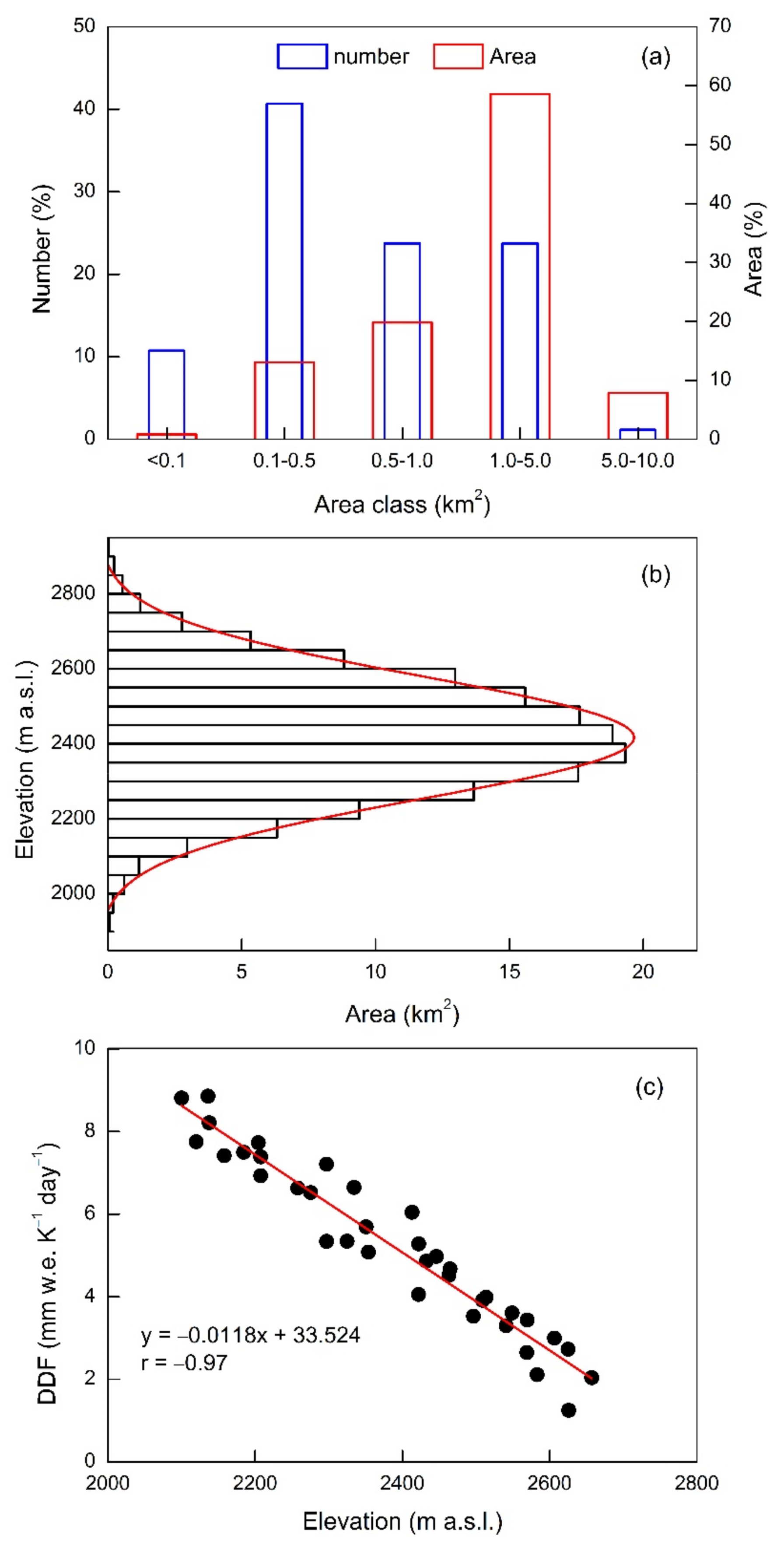
The SKMs (62.0–63.0°N, 140–142°E; Figure 1) are located in the northeastern Siberian subarctic, which extends for more than 500 km from northwest to southeast, with the highest peak being Mt. Mus-Khaya (2959 m a.s.l.). The mountain range contains a total glacier area of 210.0 km2 [7], representing ~13% of the total area of all Siberian glaciers. Glaciers in the size class of 1.0–5.0 km2 account for 58.6% of the total glacier area in the SKMs, while glaciers in the size class <0.5 km2 dominate in terms of total number (Figure 2a). Glacier elevation ranges between 1900 and 2960 m a.s.l., and more than 80% of the glacier area is concentrated from 2000 to 2600 m a.s.l. (Figure 2b). The equilibrium line altitude (ELA) varies from 2200 to 2500 m a.s.l. [7]. Glacier No. 31, which is situated in the central massif of the SKMs (Figure 1), has been extensively studied. Its area is ~3.2 km2 and its elevation varies from 2025 to 2778 m a.s.l. [7]. The glacier has experienced continuous retreat and mass loss since the middle of the 20th century [11,13,14].
A significant temperature inversion is observed in the SKMs during winter due to the Siberian High, and precipitation increases with altitude [7]. Meteorological observations, recorded at an altitude of 2446 m a.s.l. on Glacier No. 31 during 2012–2014, showed that the mean and minimum air temperatures were −13.9 and −46.0 °C, respectively, while the accumulated precipitation for one year was 342.0 mm year−1 [8]. Most of the snowfall events occur during the months of spring, summer, and early autumn [8,13,16]. Like other Arctic regions, a significant temperature rise has been observed in the SKMs, especially during winter [1,2].
The first detailed meteorological and glaciological measurements were conducted in the SKM glaciers during the 1957–1958 IGY [7]. Intermittent monitoring activities were conducted on these glaciers in the following decades [9,10,13]. The SKM glaciers were resurveyed in the summer of 2001 [10], while one-year observations were conducted in the mountain range and surroundings from August 2004 to August 2005 using meteorological instruments and ablation stakes [13]. In recent years, continuous glacier monitoring activities have been conducted on SKM glaciers under different initiatives [8,15], which have attempted to re-establish a glacier monitoring system. For instance, Takeuchi and others [15] conducted field measurements of surface melt, reflectivity, impurity features, and their associated impacts on Glacier No. 31 during the summer of 2014. An extensive monitoring system was established on Glacier No. 31 and adjacent glaciers during 2011–2014, including meteorology, glacier mass balance, and dynamic processes [8].
Glacier changes in the mountain range over various periods have been studied using field observations, remote sensing data, topographic maps, and aerial imagery [11,12,13], which have revealed marked differences in glacier retreat within the mountain range. About 19.3% of the glacier area in the mountain range was lost over the period of 1945–2003, which was estimated using satellite imagery and glacier inventories [13]. Galanin and others [12] found that the termini of Glaciers No. 29 and No. 31 retreated by 500~650 m, and the total glacier area was reduced by ~36% over the period of 1957–2012.
Most glaciological studies conducted in the mountain range have been performed on Glacier No. 31 (Figure 1). The first detailed three-year SMB measurements revealed an SMB of −0.13 m water equivalents (w.e.) year−1 during the period 1957–1959 [7]. Yamada and others [10] observed intensive melting on the whole glacier and estimated a terminus shrinkage of approximately 200 m between 1957 and 2001. Based on short-term ablation stake measurements, Takeuchi and others [15] found that the growth of ice algae on the ice surface accelerated ice melting, and the melting rate was largely higher compared to the bare ice without impurities. Zhang and others [15] estimated a total mass loss of 22.3 m w.e. over the past 64 years.
Using global position system (GPS) measurements for the period 2013–2014, Shirakawa and others [8] calculated the surface velocities of Glacier No. 31 and found a significant decreasing trend compared to measurements made during the 1957–1958 IGY. In particular, surface velocities in the middle of theglacier were larger than those in the upper and lower areas [8]. Radio-echo sounding revealed that the maximum ice thickness was ~201 m at the most upstream part of Glacier No. 31 [8].
2.2. Data
The glacier SMB model requires information about area, length, and elevation range for each glacier. The model is driven using daily meteorological variables from global climate datasets and GCM outputs. Mass balance data observed during different periods and existing estimates from previous studies were used to assess the model performance. Here, we present detailed information regarding these datasets.
The glacier information over different periods required for our modeling approach was obtained from the enlarged version of the World Glacier Inventory (WGI) [18] and the Randolph Glacier Inventory version 4.0 (RGI4.0) (GLIMS, Boulder, CO, USA) [19]. For some glaciers, there was a lack of elevation information; therefore, we derived glacier hypsometry from glacier outlines and Advanced Spaceborne Thermal Emission and Reflection Radiometer (ASTER) GDEM2.0 (NASA, Washington, DC, USA) [20]. In total, our study selected 177 glaciers for the model simulation, the total area of which was 194.0 km2. Each glacier in the mountain range was discretized into surface elevation bands of 50 m.
Direct ablation measurements were available for five glaciers (Glacier Nos. 29–33) in the mountain range. The data were observed from July 2012 to August 2013 using ablation stakes placed on these glaciers (Figure 1b). We used the ablation measurements to compute the model parameters. A summary of available observations in the mountain range is provided in Table 1. Three-year SMB data (Table 1), observed on Glacier No. 31 during the 1957–1959 IGY [7], were used for the model validation, which included annual and vertical balance profiles. In addition, two SMB time series of Glacier No. 31 for the periods of 1957–1969 and 1951–2011, derived from previous literature [14,21], were used in the model validation.
The retrospective SMB simulation for the period 1950–2011 was driven by daily air temperature and precipitation from an extended version of the observation-based global climate dataset with a resolution of 0.5° [22,23]. The data for each glacier were obtained from the grid cell nearest to the center coordinate of the glacier. This dataset was used to force glacier SMB simulations in different regions [24,25,26]. The details of the dataset mentioned above were given by Hirabayashi and others [22,23]. The future SMB projection was driven by outputs of the 12 GCMs that participated in the Coupled Model Intercomparison Project Phase 5 (CMIP5) [27]. Future simulations (2006–2100) of CMIP5 GCMs were forced by two representative concentration pathway scenarios (RCP4.5 and RCP8.5). RCP4.5 is a moderate scenario that features an increase in radiative forcing of 4.5 W m−2 by 2100 relative to the value during the pre-industrial period, while RCP8.5 is a high-emissions business-as-usual scenario that features an increase in radiative forcing of 8.5 W m−2 by 2100 [28]. The outputs of the 12 GCMs were interpolated from the original resolution (Table 2) onto a common grid (0.5° resolution) using bilinear interpolation.
To bias-correct the global climate dataset and CMIP5 GCM outputs, we used temperature and precipitation data taken from the climatic research unit (CRU) CL 2.0 dataset [29] nearest to the glacier. The CRU dataset contains mean monthly data with a 10-min spatial resolution, which is based on station data for the period 1961–1990 interpolated as a function of longitude, latitude, and elevation above sea level using the thin-plate spline method. A more detailed description of the CRU CL 2.0 dataset was given by New and others [29].
In addition, meteorological data observed from two automatic weather stations (AWSes) located on Glacier No. 31 during different periods (Figure 1 and Table 1) were used in this study. AWS data observed from August 2004 to August 2005 were used for model validation, while data observed from July 2012 to August 2013 were used for model calculation. To analyze long-term climate variations in the mountain range, we used a precipitation and air temperature dataset for the period of 1950–2014, which was obtained from the Oymyakon Station (740 m a.s.l.; Figure 1), which is near Glacier No. 31.
2.3. SMB Model
2.3.1. Model Description
We used a temperature index-based SMB model to compute the SMB for each individual glacier in the SKM. The model was run for every elevation band of the glacier, with daily time steps based on air temperature and precipitation series. This computed all major SMB components (i.e., surface melt, snow accumulation, and refreezing) described in the following sections and the associated geometric changes. All parameters of the SMB model are summarized in Table 3.
In the model, a temperature threshold approach was used to compute snow accumulation. In this approach, we applied a threshold temperature (Ttht) to differentiate snow from rain at every elevation band. Tair ≤ Ttht − 1 °C implies that precipitation falls as snow, whereas precipitation at Tair ≥ Ttht + 1 °C is rain: within this temperature range, the percentage contribution of snow and rain to total percentage is linearly interpolated. A classic temperature index model was employed to compute snow and ice melt, which linearly relates the melt rate to positive Tair [30,31]. Therefore, snow and ice melt (M) is calculated as
Note that surface melting is not equal to mass loss for a glacier due to the refreezing process [32,33,34]. To consider the effect of this process, the refreezing of meltwater and rain was estimated by considering the conduction of heat conduction into the ice and the snow layer and the presence of water at the interface between the snow layer and ice. We also considered the refreezing amount during cooling events in winter, during which the snow layer can retain up to 5% of its water content in volume. A more detailed description of this approach was reported in previous literature [26,32]. The possible amount of refreezing (RF) in each elevation band is therefore given by
Changes in glacier volume, surface area, and elevation range are affected by variations in SMB, which are estimated through volume–area and volume–length scaling [35,36]. The volume (V) of a glacier is related to its surface area (A) and its length (L) via a power law:
This method has been generally used to estimate the response of glaciers to climatic forcing at different scales [5,24,25,37,38,39]. The initial volume of each SKM glacier is calculated from the surface area recorded in the WGI through volume–area scaling. Based on the modeled SMB, glacier area is updated using Equation (3), and then volume changes after each time step. Furthermore, glacier length is adjusted using Equation (4) when volume changes. Then the approach adjusts the surface area and length of the glacier in each time step based on the modeled SMB, leading to a retreat/advance of the glacier terminus. As a result, the elevation–area distribution of the glacier is updated according to these changes. Here, we calculated the glacier area of every elevation band through a normal distribution obtained from the surface area and maximum and minimum elevation ranges. This approximate estimation was based on a normal distribution of the elevation–area observed in SKM glaciers (Figure 2b).
In addition, we set snow above and bare ice below the ELA to initialize the surface type at the end of the melt season in the first year of the simulation. The surface type was then updated at every elevation band of the glacier based on a simulation of daily snowfall and melt. The full details of the glacier SMB model are available in previous studies [14,24].
2.3.2. Model Parameters
In our modeling approach, degree-day factors (DDFice and DDFsnow), temperature lapse rates (TLRs), and vertical precipitation gradients (VPGs) were needed to run the model. However, it is difficult to estimate these parameters in high-altitude regions of the SKMs, where few meteorological and glaciological data exist. Therefore, it is challenging to estimate these parameters in the mountain range, which may affect to a large degree the model performance.
Meteorological observations in the SKMs indicate complex variation in air temperatures with increasing altitude due to the strong temperature inversion in winter and the increase in precipitation with altitude [7]. Therefore, the temporal variability of the TLRs and VPGs should be considered in SMB simulations of the mountain range. A set of 12 monthly TLRs and VPGs was calculated based on meteorological observations at different elevations of Glacier No. 31, and it was validated through the data generated using monthly TLRs and VPGs against observations on the glacier [14]. Air temperature and precipitation from the grid cell closest to the glacier were extrapolated to all glacier elevation bands using these monthly TLRs and VPGs. Full details of the TLRs and VPGs and the associated validation are given in Zhang and others [14].
DDFsnow and DDFice display marked spatial variability and are generally calculated based on field observations of air temperature and glacier ablation [30,31]. In this study, the degree-day factors (DDFs) were calculated from glacier ablation and air temperature observed on Glacier Nos. 29–33 from August 2012 to August 2013 (Table 1). On average, DDFsnow and DDFice were 2.1 and 6.2 mm w.e. K−1 day−1, respectively. We found that DDFs and elevation had a significant negative correlation with a correlation coefficient (r) of −0.97 (significance level p < 0.001; Figure 2c), which indicated that the DDFs decreased with increasing elevation. This finding agrees with the results of Zhang and others [31]. In our model simulation, this relationship was applied to assign DDF values to every band of the glacier in the SKMs.
2.3.3. Model Validation
Validating a model in the SKMs remains largely challenging because of the lack of meteorological and glaciological observations on the glaciers. However, the model validation process is paramount to model performance in realistically capturing each process of SMB. Therefore, a three-step procedure was applied to validate the model performance, which relied on existing observations and previous estimates in the SKMs (Table 1).
In the first step, we validated the modeled results against observed SMB vertical profiles and previous estimates for Glacier No. 31 during 1957–1959 (Table 1). This process could assess the performance of our modeling approach to simulate the SMB variation with altitude. Then our simulations were compared to two annual SMB time series for the periods 1957–1969 and 1951–2011 from different studies [14,21]. This allowed us to assess the ability of the approach to capture the yearly variability in SMB. Finally, the overall area distribution of elevation in Glacier Nos. 29–32 (Figure 1) (which was derived from the RGI4.0 glacier outlines and ASTER GDEM2) and the rates of change in glacier area in the mountain range (which were derived from the two glacier inventories mentioned above) were used to assess the ability of our model to simulate the feedback of glacier hypsometry and the SMB.
In addition, the model performance was evaluated using R2 (determination coefficient) and mean absolute error (MAE). The MAE is defined as
in which n is the number of observations, B is the SMB, and subscripts “obs” and “mod” denote observed and modeled data. Here, the R2 value represents how well the model performs in calculating the variation in the SMB, whereas the MAE value indicates the ability of the model to capture the magnitude of the SMB.
2.3.4. Bias Correction
The forcing data used in this study, including global climate dataset and GCM outputs, contained biases that required bias correction before application to glaciers. Therefore, we applied the delta change method [40,41,42,43] to execute bias correction of these datasets while retaining their variability. The method removes biases from the meteorological variables of global climate dataset and GCM outputs through the involvement of an additive correction for temperature and a multiplicative correction for precipitation. The two correction factors were computed from 30-year (1961–1990) average monthly means of the two datasets and the CRU CL 2.0 dataset, respectively. Furthermore, the bias-corrected temperature and precipitation had the same resolution as the CRU grid cell. We then applied the two correction factors to obtain the corrected daily temperature (TCOR) and precipitation (PCOR) at the grid cell of the two datasets nearest to the glacier, which are respectively given as
3. Results
3.1. Model Evaluation against Observations and Previous Estimates
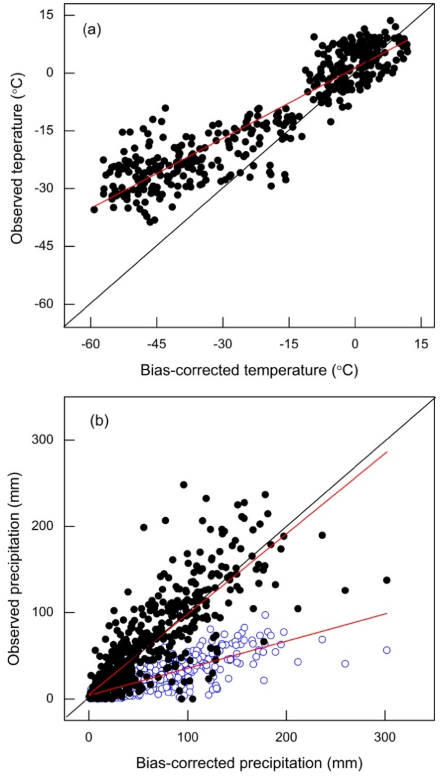
The bias-corrected results of temperature and precipitation from applying the delta change method were evaluated based on observations in the mountain range over different periods (Figure 3). We compared bias-corrected temperatures and observations recorded at the AWS of Glacier No. 31, which is situated at the glacier terminus at ~1988 m a.s.l., from August 2004 to August 2005 (Figure 1). The results indicated a close correlation between bias-corrected temperatures and AWS observations (Figure 3a), yielding an R2 of 0.85. An additional analysis of our results indicates that the bias-corrected results were unduly influenced by the lower temperatures in winter months, in which the R2 between the observed and bias-corrected temperatures was 0.49.
Unlike temperature, the bias-corrected results of monthly precipitation overestimated the monthly observations recorded at the Oymyakon Station for the period 1950–2011 (Figure 3b), possibly due to the large elevation difference (1500 m) between the Oymyakon Station and the grid cell. The R2 and MAE values between the bias-corrected monthly precipitation and observations were 0.64 and 27.0 mm, respectively. To consider the effect of elevation differences, we generated the monthly precipitation from the Oymyakon Station using the VPGs, for which its elevation was the same as in the bias-corrected dataset. As shown in Figure 3b, the bias-corrected precipitation captured the observation-based generated results well, for which the R2 and MAE values were 0.72 and 15.0 mm, respectively. Thus, the bias-corrected results were in good agreement with the observed data, which were good enough to be used as forcing data for the SMB model in the SKMs.
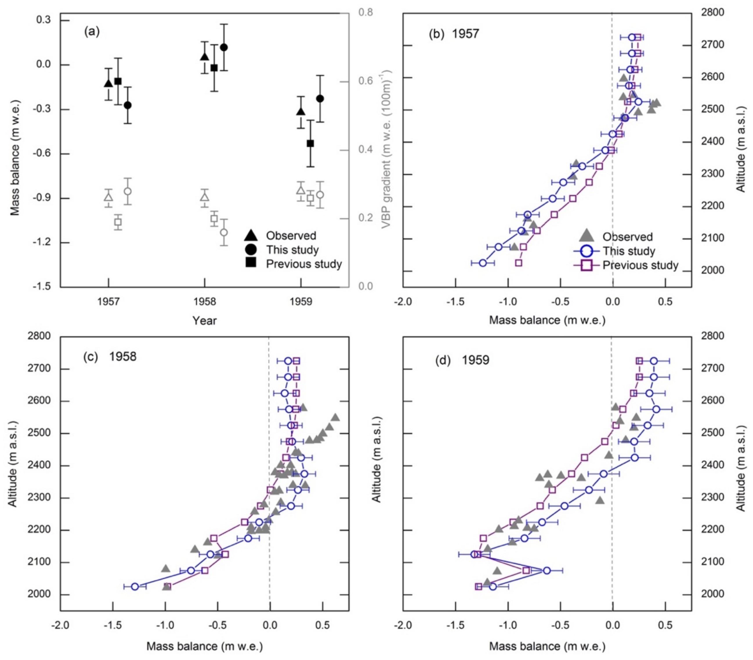
We assessed model performance by comparing the observed mean SMB of Glacier No. 31 to the modeled results for the period 1957–1959 and by comparing observed and modeled vertical balance profiles (VBPs) and associated gradients (Figure 4). We calculated the SMB and VBPs for the period for which observed data were available based on the bias-corrected air temperature and precipitation series and estimated parameters. There was close agreement between the observed, previously estimated, and modeled results in the corresponding period (Figure 4a), which was the primary objective of our model simulation. As shown in Figure 4a, although a discrepancy between the modeled results and the observations/previous estimates existed, observations/previous estimates fell within one standard error of the modeled results. Overall, the modeled values matched the observations/previous estimates well, which was very important, as the area-integrated mass was the primary interest in our study. For all other cases, the modeled, observed, and previously estimated VBPs agreed well within the error ranges (Figure 4b–d). This gave us confidence in the model’s ability to capture the vertical structure of observed SMB within the glacier altitude range in the SKMs.
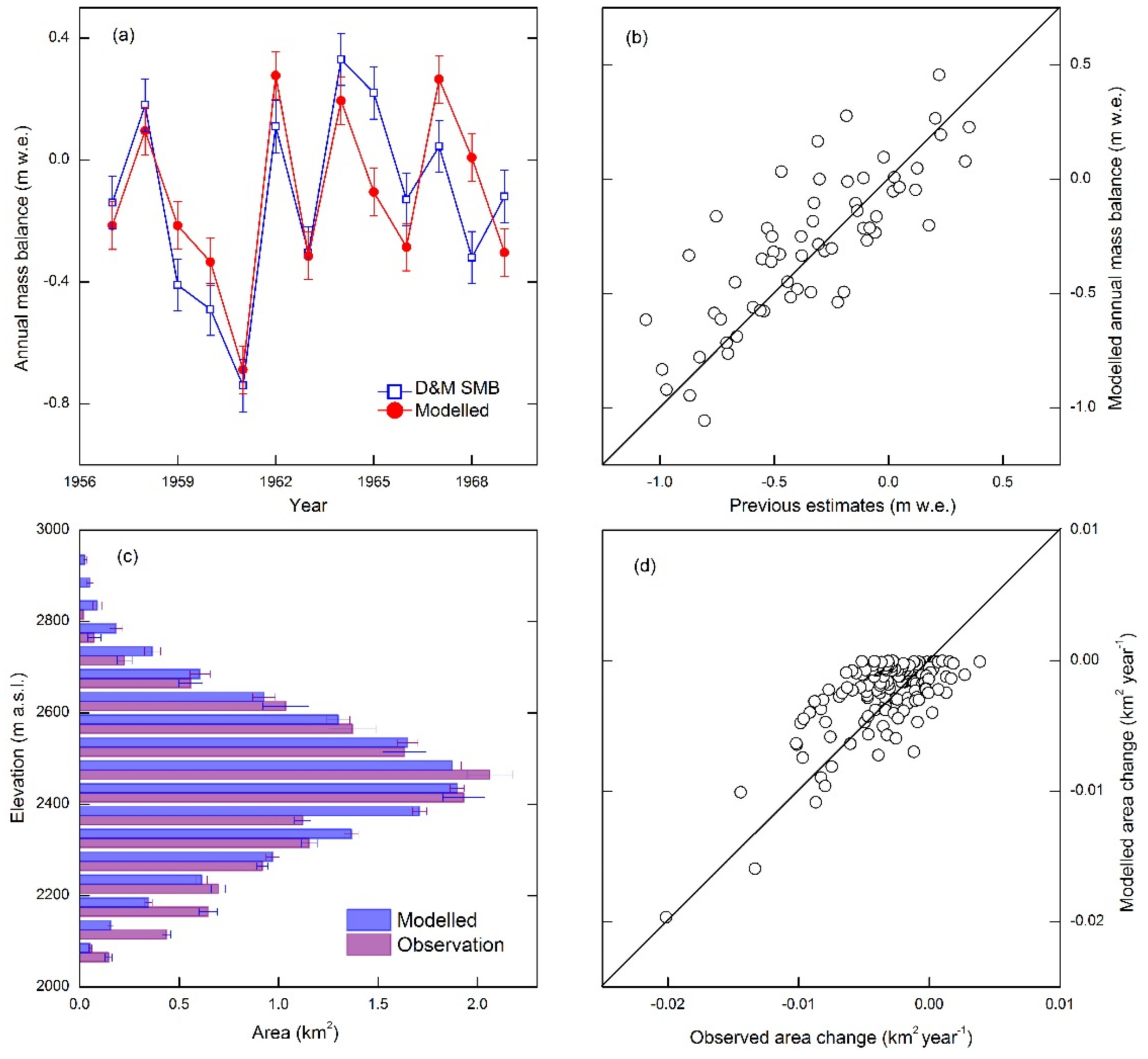
Similarly, the model performed reasonably well in terms of the long-term variation in the annual SMB on Glacier No. 31 (Figure 5). Generally, our simulations and previous results [14,21] demonstrated a consistent long-term variation over the periods 1957–1969 and 1951–2011, respectively. The variation in modeled SMB captured the estimates of 1957–1969 well (Figure 5a). An analysis of 1957–1969 SMB values indicated that the R2 and the MAE were 0.64 and 0.15 m w.e., respectively. A comparison between modeled SMB and the estimates over the period 1951–2011 showed similar variability (Figure 5b), yielding an R2 value of 0.66 and an MAE value of 0.16 m w.e. In total, the mean modeled SMB of Glacier No. 31 was −0.30 m w.e. during 1951–2011, which was slightly lower compared to the previous estimate for the same period (−0.34 m w.e.) [14].
As a further model validation, the overall surface area distribution with altitude for Glacier Nos. 29–32 (Figure 1) (derived from RGI4.0 glacier outlines and ASTER GDEM2) was compared to the results estimated using our modeling approach for the period 1951–2003 (Figure 5c). In the comparison, the R2 and MAE values were 0.85 and 0.14 km2 for all elevation bands, respectively. Furthermore, a dataset of change rates of glacier area in the mountain range for the period 1951–2003, estimated based on the two glacier inventories (hereafter, observed rates), were compared to the results modeled for the period 1951–2003 (Figure 5d). It was found that the modeled and observed rates of change in area for most cases matched well, for which the R2 and MAE values were respectively 0.52 and 0.002 km2 year−1. The overall mean decreasing rate in glacier area for the whole mountain range was 0.56 km2 year−1, slightly less than the observation of 0.63 km2 year−1 for the period 1951–2003. A comparison of the two independent approaches suggested that our modeling approach was sufficient for modeling the feedback of SMB and the change in glacier hypsometry.
3.2. Spatiotemporal Variability in the SMB
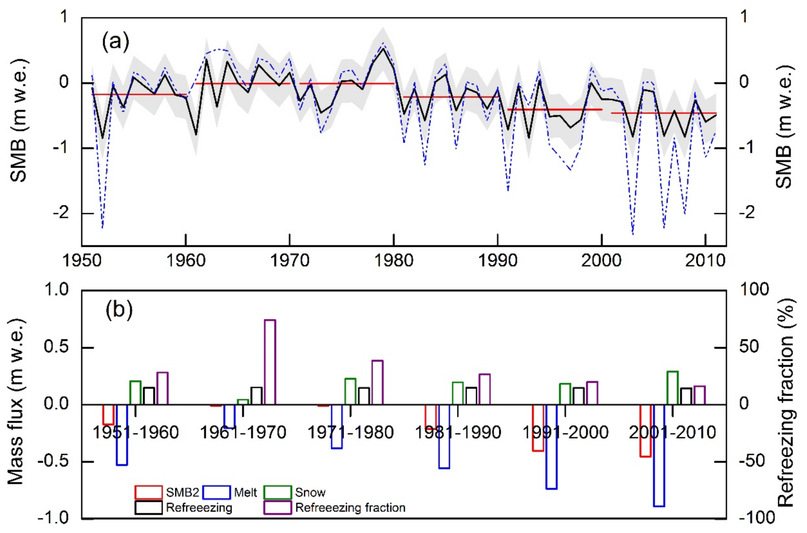
Modeled SMB variation for the SKM glaciers is shown in Figure 6a. The mean annual SMB of SKM glaciers between 1951 and 2011 was −0.22 m w.e. year−1. A large interannual SMB variation was observed (Figure 6a), with a maximum value of +0.53 m w.e. in the balance year of 1977/1978 and a minimum value of −0.84 m w.e. in the 1952/1953 year. Overall, a slightly negative SMB was found before 1991, and then rapidly increasing mass loss was observed (Figure 6a).
The SMB of SKM glaciers was slightly negative in the 1950s and almost balanced between the 1960s and the 1980s, and then it evolved into a strong disequilibrium after the 1990s (Figure 6). For the period 1991–2011, the mean mass loss rate was –0.43 m w.e. year−1, which was about four times the loss rate during 1951–1990 (−0.10 m w.e. year−1). This implies that glaciers in the SKMs have undergone rapid mass loss since 1991 (Figure 6). A similar trend was observed in the cumulative glacier SMB for the whole mountain range. The overall cumulative SMB was –13.1 m w.e. during 1951–2011, ~69% of which was observed from 1991 to 2011.
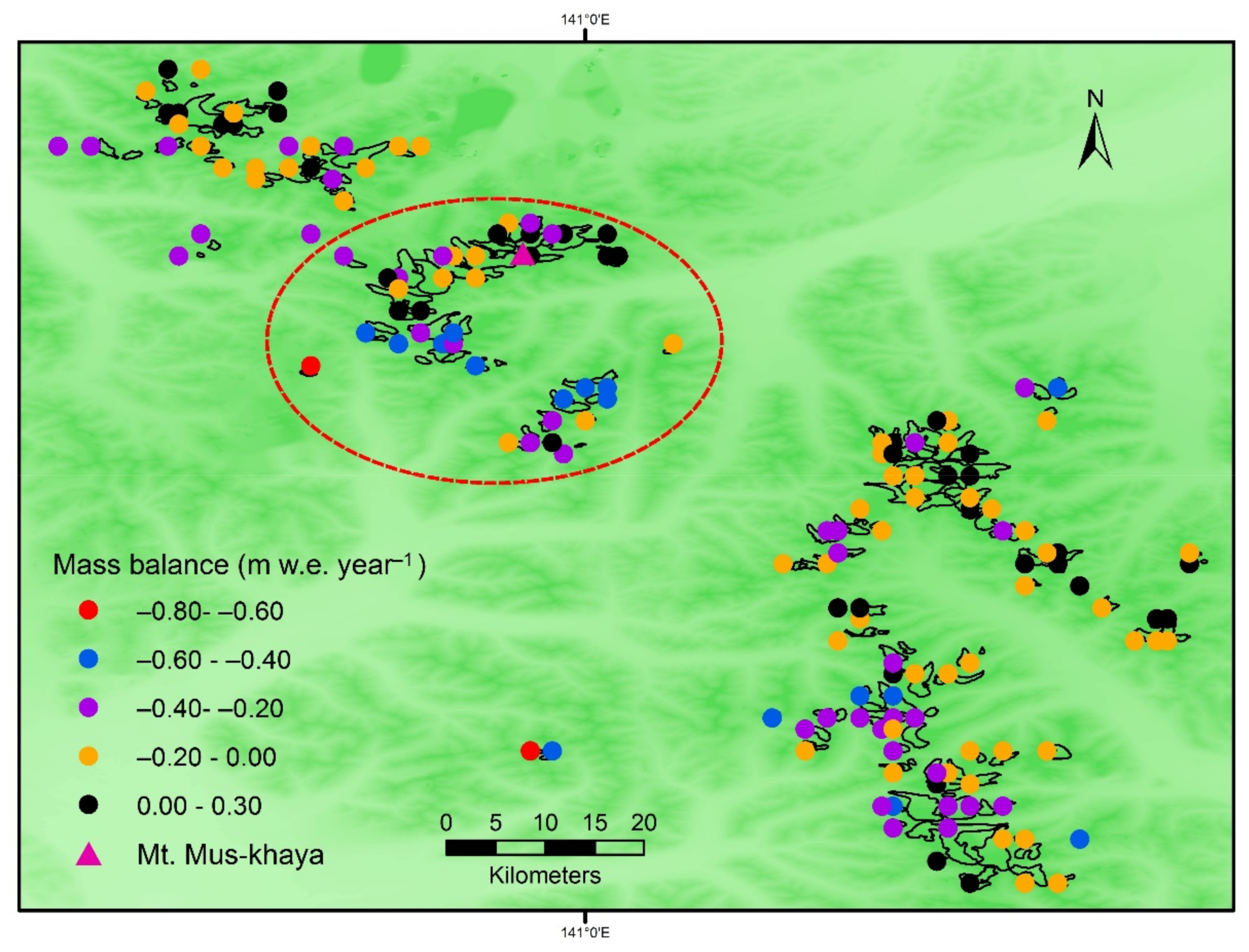
Of all SKM glaciers, 77.4% experienced mass loss between 1951 and 2011, representing ~83.0% of the overall surface area of SKM glaciers. We found considerable variability in the SMB among the individual glaciers over the study period (Figure 7). The mountain range was separated into three regions (northern, central, and southern) based on the location of the highest peak of Mt. Mus-Khaya (Figure 7). Glaciers in the central region of the mountain range experienced the highest rate of mass loss during the study period (−0.19 m w.e. year−1), while glaciers in the northern and southern regions underwent lower rates of mass loss or slight mass gains, with a mean rate of mass loss of −0.13 m w.e. year−1. For the glaciers in the northern and southern regions, the overall surface area represented 72.0% of the total glacier area. In particular, a slightly positive mass balance was observed on 20.4% of the glaciers in the southern region between 1951 and 2011, with a mean loss rate of −0.11 m w.e. year−1.
4. Discussion
4.1. Drivers of Regional Mass Loss
Analyzing the components of the mass budget is vital for a better understanding of the drivers of glacier mass change in the mountain range. Before 1991, the Suntar-Khayata glaciers experienced a slight mass loss trend (Figure 6), with a nonsignificant trend of −1.5 mm w.e. year−1. In terms of the SMB components (Figure 6b), glacier melt persistently and significantly exceeded snow accumulation during the period considered in this study. This indicates the importance of the refreezing process to the Suntar-Khayata glaciers. The mass-retaining effect of refreezing maintained a low mass loss from the glaciers before 1991 (Figure 6b). Our analysis indicated that the refreezing fraction (refreezing/melt) was 36.0% between 1951 and 1990.
Between 1991 and 2011, the SKM glaciers experienced a significant increase in mass loss (Figure 6), resulting in an average loss of –0.43 m w.e. year−1 over this period. Concerning the SMB components, modeled surface melt and snow accumulation increased at rates of 15.4 and 4.5 mm w.e. year−1, respectively, while refreezing decreased slightly (Figure 6b). Although the modeled accumulation displayed an increasing trend during the study period, the trend in SMB was almost exclusively driven by increased surface melt, as shown unambiguously in Figure 6b. Compared to the period before 1991, surface melt increased by 95.0%, while the refreezing fraction was 18.0% between 1991 and 2011, much smaller than before 1991.
Temperature strongly influenced the processes controlling the mass budget components [6]. Arctic Monitoring and Assessment Programme (AMAP) [2] has reported that Siberian glaciers are decreasing in area in response to summer temperature increases and a relatively small snowfall increase. Observations at the Oymyakon Station (Figure 1) indicated that the annual precipitation changed nonsignificantly over the period 1950–2014, while air temperature increased at a rate of 0.4 °C (10 year)−1. In recent years (1991–2014), monthly temperatures at the beginning and end of the melt seasons have risen by 1.6 and 2.3 °C, respectively, relative to the averages during 1950–1990. In particular, a large increase of more than 2 °C since 1960 has occurred in the Arctic regions, including the SKM, during the cold season (November–April) [2]. There is growing evidence that temperature rise in high-altitude environments is faster than in low-altitude regions [44]. Consequently, the glacier system in the SKMs is experiencing a more rapid temperature change than lower-altitude stations are (e.g., Oymyakon Station). Such warming, especially during the cold season, can prolong the melt period, change the snow/rain ratio and snow albedo feedback, and reduce the refreezing capacity on SKM glaciers. This highlights the vulnerability of glaciers in the SKM to temperature changes.
4.2. Future Variations in the SMB
Warming trends will continue in the Arctic, where the temperatures are projected to increase about 1.7–3.1 °C and 3.8–6.0 °C by the end of this century under two scenarios (RCP4.5 and RCP8.5), respectively, relative to pre-industrial levels [2]. These projected values are higher than the 1.5 °C goal proposed in the Paris Agreement of 2015. The projected increase in precipitation from the CMIP5 GCMs shows a greater increase percentage in the Arctic than in elsewhere in the Northern Hemisphere, although the precipitation totals are relatively small [2,45]. In the coming decades of this century, the Arctic’s climate will shift to a new state [2], strongly affecting the status of Arctic glaciers.
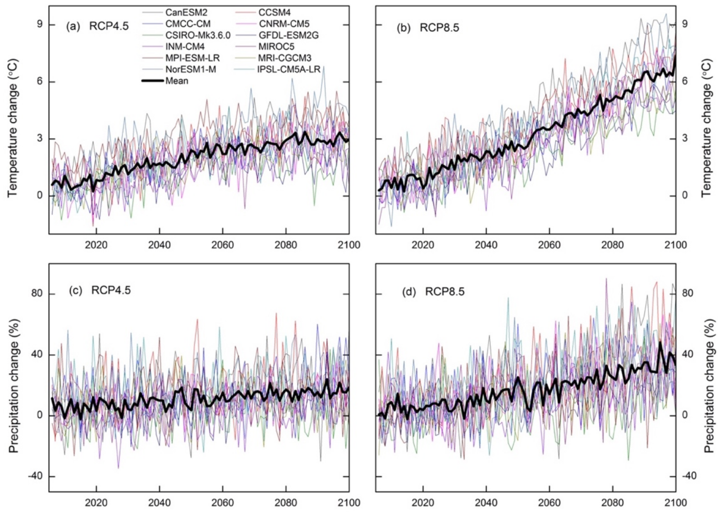
In the SKMs, significant warming is projected from the 12 CMIP5 GCMs for RCP4.5 and RCP8.5 in the coming decades (Figure 8a,b), while the precipitation projected by the GCMs reveals significant variability with a slight increasing trend (Figure 8c,d). Compared to the 1986–2005 averages, the temperature projections for RCP4.5 and RCP8.5 show respective warming rates of 0.03 and 0.07 °C year−1 by 2100 (Figure 9a,b), whereas the precipitation projections for RCP4.5 and RCP8.5 indicate respective increasing rates of 0.13% year−1 and 0.35% year−1 (Figure 8c,d). For 2071–2100, the projected warming for RCP4.5 and RCP8.5 in the SKMs exceeds 2.5 and 5.5 °C relative to the 1986–2005 average, while precipitation is projected to increase by 13.5% and 27.4%, respectively.
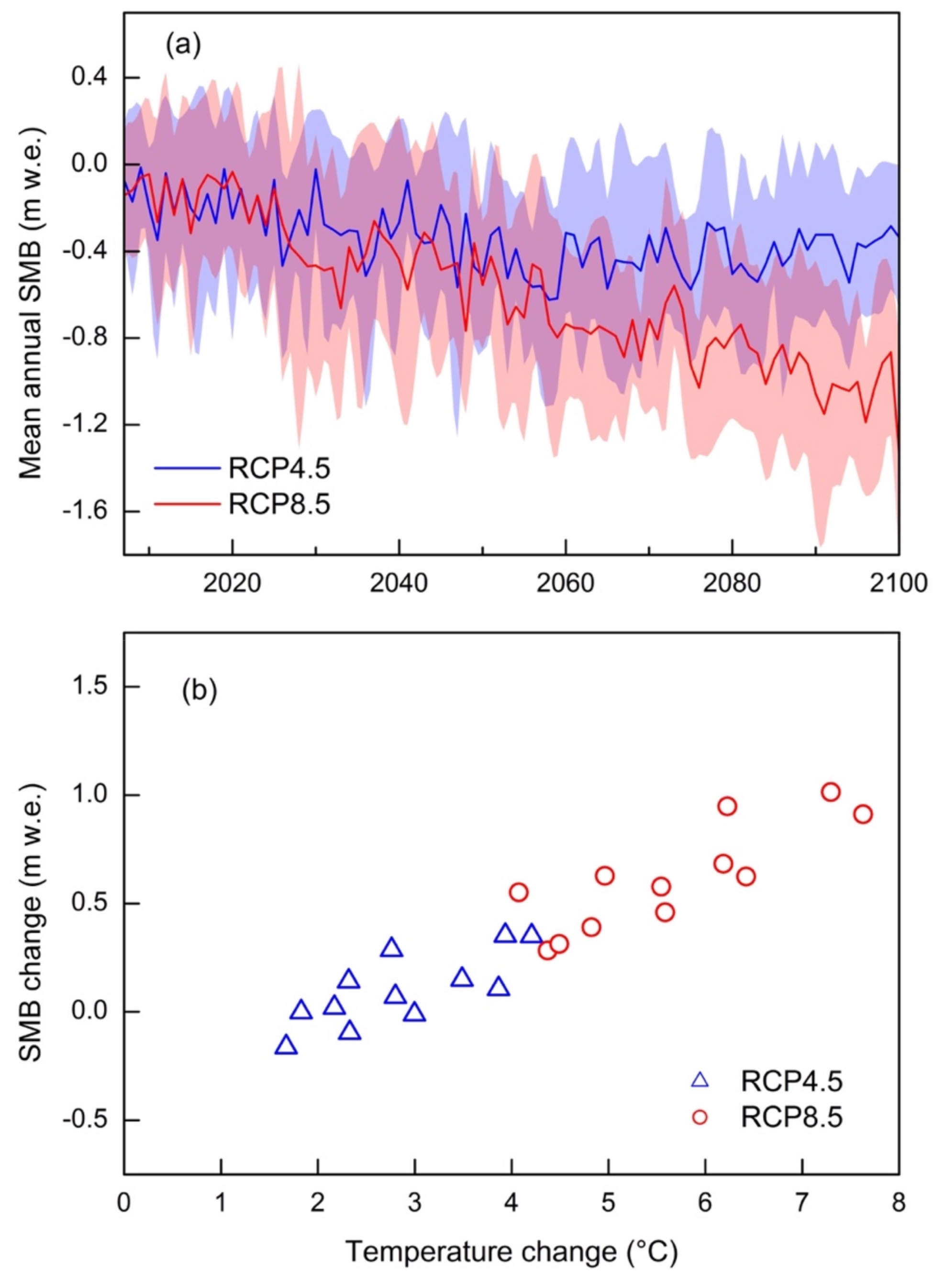
To estimate the response of the Suntar-Khayata glaciers to future temperature and precipitation conditions, the SMB for all SKM glaciers was calculated by rerunning the model, which was forced using bias-corrected data from the 12 CMIP5 GCMs for the two scenarios. The simulations showed a continuous mass loss for the SKMs in the following decades under the two RCPs (Figure 9a). The pronounced differences in projected glacier mass loss between RCP4.5 and RCP8.5 become larger in the second half of the century (Figure 9a). For the RCP4.5 scenario, the projected mass loss increases progressively and becomes relatively stable by the end of the century (Figure 9a), while it increases for the RCP8.5 scenario.
Although precipitation is projected to increase (Figure 8c,d), this increase will be insufficient to compensate for the increased surface melt resulting from temperature rise. During 2071–2100, the projected surface melt under the two RCPs increases by ~48% (RCP4.5) and ~185% (RCP8.5) relative to the 1986–2005 average. As a consequence, the annual SMB of the mountain range for RCP8.5 is about −0.92 m w.e. during 2071–2100, more negative compared to the RCP4.5 scenario (−0.40 m w.e.). In the RCP8.5 scenario, 50% ± 7% of the total glacier area is projected to remain for the whole mountain range over the period 2071–2100, while 70% ± 4% of the total area will remain in the RCP4.5 scenario. In addition, the projected temperature change and mass loss appear to be a nearly linear relationship (Figure 9b). This implies that compared to the 1986–2005 average, most projections from the CMIP5 GCMs lead to much larger warming and more loss of glacier mass in the SKMs of the northeastern Siberian subarctic.
4.3. Uncertainties in the SMB Calculation
In addition to modeling approaches, two other approaches are generally used to calculate glacier mass balance on a regional scale: geodetic and glaciological methods [6]. The geodetic method has been mostly used to estimate short-term recent glacier mass changes, but it cannot provide information on annual and seasonal patterns of mass changes. In contrast, the glaciological method, which estimates SMB from the extrapolation of in situ mass balance measurements, generally has good temporal but poor regional coverage. In this study, a modeling approach was applied to calculate the glacier SMB in the SKMs, with the aim of enhancing our understanding of the long-term mass variability of glaciers on a regional scale. In our modeling approach, uncertainties in the SMB simulation arose mainly from forcing the data and the determination of model parameters.
The accuracy of the forcing data is a great challenge for glacier SMB modeling at the regional scale, and it is considered to be one of the main sources of uncertainty in SMB studies [38,39,44,46,47]. To remove the biases of the gridded datasets used in this study, we used the delta change approach to bias-correct the global climate dataset and GCM outputs by means of the CRU dataset. This method has been widely used in different regions and has performed well [41,42,43,44]. However, large differences in the amount and number of wet days exist between the global climate dataset and GCM outputs and observed precipitation [43,44]. These differences could have led to bias-corrected precipitation in this study that contained unrealistic peaks. This difficulty has not yet been resolved due to the limited observed daily data available in mountainous regions. Although the influence of such uncertainty in precipitation on SMB simulations may not have been fully resolved, our analysis indicated good agreement between the bias-corrected precipitation and long-term observations (Figure 3b). In particular, using the bias-corrected temperature and precipitation, our model could accurately reproduce the observed SMB profiles (Figure 4).
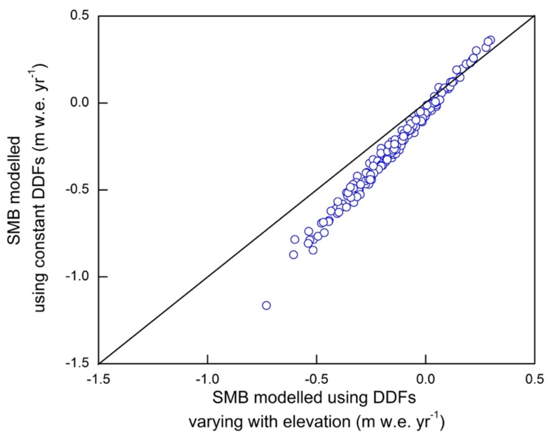
For regional SMB modeling, one challenge is the determination of model parameters for each individual glacier. Among the parameters inquired into in our modeling approach, DDFsnow and DDFice were assigned to each elevation band of each individual glacier using the relationship between DDFs and elevation (Figure 2c), which was established based on ablation measurements of the five glaciers (Figure 1). As shown in Figure 2c, the estimated DDFs varied significantly with elevation on these glaciers. In previous studies that have conducted regional/global SMB simulations, DDFsnow and DDFice were generally assigned for each glacier or region and were held spatially constant [24,25,39,44,46]. Previous studies have reported that DDFs exhibit marked spatial variability [30,31]. To quantify the importance of the spatial characteristics of the DDFs for SMB modeling, the SMB of SKM glaciers was recalculated by running our modeling approach, with constant DDFs for each individual glacier, and their spatial variation with elevation were not considered. The results indicated that spatial variability in the DDFs strongly affected glacier SMB (Figure 6a and Figure 10). Compared to the simulation considering spatial variability in the DDFs, running the model using constant DDFs for each glacier resulted in a higher mass loss for all glaciers (Figure 10). In total, the regional rate of glacier mass loss in the simulation using constant DDFs increased by approximately 46% compared to the simulation considering spatial characteristics of the DDFs. Therefore, our experiment indicated the importance of the spatial variability of DDFs in SMB simulations at the regional scale, which was considered in our modeling approach.
5. Conclusions
In this study, we analyzed spatiotemporal variability in glacier SMB over the SKMs of the northeastern Siberian subarctic, simulated by a temperature index SMB model that accounted for individual components of the glacier mass budget. Our model results were cross-validated well during the period for which observations and previous estimates were simultaneously available in the region, confirming the predicative ability of the model for SMB modeling.
Our analysis indicated a large interannual SMB variation in the SKMs over the 61-year period from 1951 to 2011, with a mean annual value of −0.22 m w.e. year−1. Two contrasting variation trends in SMB were found in the mountain range: a slightly negative balance before 1991 and a significantly rapid mass loss after 1991. The mean annual SMB for 1991–2011 (−0.43 m w.e. year−1) was about four times that for 1951–1990 (−0.10 m w.e. year−1). We detected marked variability in the SMB between individual glaciers over the study period, with glaciers in the central region of the SKMs experiencing the highest mass loss rates and relatively low mass loss rates or slight mass gains in the northern and southern regions.
Compared to before 1991, surface melt increased by 95.0%, while the refreezing fraction largely decreased between 1991 and 2011. This reflected the importance of surface melt, which was substantially impacted by temperature changes, for the annual mass budget in the SKM. For 2071–2100, the temperature change projected by the CMIP5 GCMs exceeded 2.5 °C for two RCP scenarios compared to the 1986–2005 average. In response to such an increase in temperature, 30% and 50% of the total present glacier area in the mountain range would be lost for the period 2071–2100 in the RCP4.5 and RCP8.5 scenarios, respectively.
This study provides a complete picture of the glacier mass change in the SKMs, for which meteorological and glaciological observations scarcely exist. The results fill the knowledge gaps regarding the glacier–climate relationship and its associated impacts in the mountain range. Our study specifically provides a basis for better understanding the drivers of regional mass loss and for obtaining better projections under different climate scenarios in the SKMs.
Author Contributions
Conceptualization, Y.Z., H.E., and T.O.; methodology, Y.Z.; software, Y.Z and Z.J.; validation, Y.Z., J.W., and X.W.; formal analysis, Y.Z.; resources, Y.Z., H.E., and T.O.; data curation, Y.Z. and H.E.; writing—original draft preparation, Y.Z.; writing—review and editing, X.W.; visualization, Y.Z.; supervision, Y.Z. and X.W.; project administration, Y.Z., X.W., and Z.J.; funding acquisition, Y.Z., X.W., J.W., and Z.J.
Funding
This research was funded by the NSFC (Grant Nos. 41671057, 41761144075,41771075, and 41471067), the MOST Program (Grant No. 2013FY111400), and the CAS Major Project (Grant No. KZZD-EW-12-1).
Acknowledgments
We would like to thank the following departments for providing the datasets used in this study: the Arctic Data Archive System of the National Institute of Polar Research, the RGI Consortium, and CMIP5.
Conflicts of Interest
The authors declare no conflicts of interest.
References
- Arctic Monitoring and Assessment Programme (AMAP). Snow, Water, Ice and Permafrost in the Arctic (SWIPA): Climate Change and the Cryosphere; Arctic Monitoring and Assessment Programme (AMAP): Oslo, Norway, 2011. [Google Scholar]
- Arctic Monitoring and Assessment Programme (AMAP). Snow, Water, Ice and Permafrost in the Arctic (SWIPA) 2017; Arctic Monitoring and Assessment Programme (AMAP): Oslo, Norway, 2017. [Google Scholar]
- Serreze, M.C.; Barry, R.G. Processes and impacts of Arctic amplification: A research synthesis. Glob. Planet. Chang. 2011, 77, 85–96. [Google Scholar] [CrossRef]
- Church, J.A.; Clark, P.U.; Cazenave, A.; Gregory, J.M.; Jevrejeva, S.; Levermann, A.; Merrifield, M.A.; Milne, G.A.; Nerem, R.S.; Nunn, P.D.; et al. Sea Level Change. In Climate Change 2013: The Physical Science Basis; Stocker, T.F., Qin, D., Plattner, G.-K., Tignor, M., Allen, S.K., Boschung, J., Nauels, A., Xia, Y., Bex, V., Midgley, P.M., Eds.; Cambridge University Press: Cambridge, UK; New York, NY, USA, 2013. [Google Scholar]
- Marzeion, B.; Jarosch, A.H.; Gregory, J.M. Feedbacks and mechanisms affecting the global sensitivity of glaciers to climate change. Cryosphere 2014, 8, 59–71. [Google Scholar] [CrossRef] [Green Version]
- Cuffey, K.M.; Paterson, W.S.B. The Physics of Glaciers, 4th ed.; Butterworth-Heinemann: Oxford, UK, 2010. [Google Scholar]
- Koreisha, M.M. Present Glaciers of the Suntar-Khayata Range; Nauka: Moscow, Russia, 1963. [Google Scholar]
- Shirakawa, T.; Kadota, T.; Fedorov, A.; Konstantinov, P.; Suzuki, T.; Yabuki, H.; Nakazawa, F.; Tanaka, S.; Miyairi, M.; Fujisawa, Y.; et al. Meteorological and glaciological observations at Suntar-Khayata Glacier No. 31, east Siberia, from 2012–2014. Bull. Glaciol. Res. 2016, 34, 33–40. [Google Scholar] [CrossRef]
- Vinogradov, O.N. New data about modern and former glaciation of Suntar Khayata (in Russian). Data Glaciol. Study 1972, 19, 80–91. [Google Scholar]
- Yamada, T.; Takahashi, S.; Shiraiwa, T.; Fujii, Y.; Kononov, Y.; Ananicheva, M.D.; Koreisha, M.M.; Muravyev, Y.D.; Samborsky, T. Reconnaissance on the No. 31 Glacier in the Suntar-Khayata Range, Sakha Republic, Russian Federation. Bull. Glaciol. Res. 2002, 19, 101–106. [Google Scholar]
- Ananicheva, M.D.; Koreisha, M.M.; Takahashi, S. Assessment of glacier shrinkage from the maximum in the Little Ice Age in the Suntar-Khayata Range, North-East Siberia. Bull. Glaciol. Res. 2005, 22, 9–17. [Google Scholar]
- Galanin, A.A.; Lytkin, V.M.; Fedorov, A.N.; Kadota, T. Recession of glaciers in the Suntar-Khayata Mountains and methodological consideration of its assessment. Ice Snow 2013, 53, 30–42. [Google Scholar] [CrossRef]
- Takahashi, S.; Sugiura, K.; Kameda, T.; Enomoto, H.; Kononov, Y.; Ananicheva, M.D.; Kapustin, G. Response of glaciers in the Suntar-Khayata range, eastern Siberia, to climate change. Ann. Glaciol. 2011, 52, 185–192. [Google Scholar] [CrossRef]
- Zhang, Y.; Enomoto, H.; Ohata, T.; Katota, T.; Shirakawa, T.; Takeuchi, N. Surface mass balance on Glacier No. 31 in the Suntar–Khayata Range, eastern Siberia, from 1951 to 2014. J. Mt. Sci. 2017, 14, 501–512. [Google Scholar] [CrossRef]
- Takeuchi, N.; Fujisawa, Y.; Kadota, T.; Tanaka, S.; Miyairi, M.; Shirakawa, T.; Kusaka, R.; Fedorov, A.N.; Konstantinov, P.; Ohata, T. The effect of impurities on the surface melt of a glacier in the Suntar Khayata Mountain Range, Russian Siberia. Front. Earth Sci. 2015, 3, 82. [Google Scholar] [CrossRef]
- Ananicheva, M.D.; Krenke, A.N.; Barry, R.G. The Northeast Asia mountain glaciers in the near future by AOGCM scenarios. Cryosphere 2010, 44, 435–445. [Google Scholar] [CrossRef]
- Amante, C.; Eakins, B.W. ETOP1 1 Arc-Minute Global Relief Model: Procedures, Data Sources and Analysis. NOAA Technical Memorandum NESDIS NGDC-24; National Geophysical Data Center, NOAA: Boulder, CO, USA, 2009. [Google Scholar] [CrossRef]
- Cogley, J.G. A more complete version of the World Glacier Inventory. Ann. Glaciol. 2009, 50, 32–38. [Google Scholar] [CrossRef] [Green Version]
- Arendt, A.; Bliss, A.; Bolch, T.; Cogley, J.G.; Gardner, A.S.; Hagen, J.-O.; Hock, R.; Huss, M.; Kaser, G.; Kienholz, C.; et al. Randolph Glacier Inventory—A Dataset of Global Glacier Outlines: Version 4.0; Technical Report of Global Land Ice Measurements from Space (GLIMS): Boulder, CO, USA, 20 December 2014. [Google Scholar]
- Tachikawa, T.; Kaku, M.; Iwasaki, A.; Gesch, D.; Oimoen, M.; Zhang, Z.; Danielson, J.; Krieger, T.; Burtis, B.; Haase, J.; et al. ASTER Global Digital Elevation Model Version 2—Summary of Validation Results; Technical Report for NASA Land Processes Distributed Active Archive Center and the Joint Japan-US ASTER Science Team: Washington, DC, USA, January 2011. [Google Scholar]
- Dyurgerov, M.B.; Meier, M.F. Glaciers and the Changing Earth System: A 2004 Snapshot; Institute of Arctic and Alpine Research, University of Colorado at Boulder: Boulder, CO, USA, 2005; p. 58. [Google Scholar]
- Hirabayashi, Y.; Kanae, S.; Struthers, I.; Oki, T. A 100-year (1901–2000) global retrospective estimation of the terrestrial water cycle. J. Geophys. Res. 2005, 110, D19101. [Google Scholar] [CrossRef]
- Hirabayashi, Y.; Kanae, S.; Motoya, K.; Masuda, K.; Döll, P. A 59-year (1948–2006) global near-surface meteorological data set for land surface models. Part I: Development of daily forcing and assessment of precipitation intensity. Hydrol. Res. Lett. 2008, 2, 36–40. [Google Scholar] [CrossRef]
- Hirabayashi, Y.; Döll, P.; Kanae, S. Global-scale modeling of glacier mass balances for water resources assessments: Glacier mass changes between 1948 and 2006. J. Hydrol. 2010, 390, 245–256. [Google Scholar] [CrossRef]
- Hirabayashi, Y.; Zhang, Y.; Watanabe, S.; Koirala, S.; Kanae, S. Projection of glacier mass changes under a high-emission climate scenario using the global glacier model HYOGA2. Hydrol. Res. Lett. 2013, 7, 6–11. [Google Scholar] [CrossRef]
- Zhang, Y.; Hirabayashi, Y.; Liu, S. Catchment-scale reconstruction of glacier mass balance using observations and global climate data: Case study of the Hailuogou catchment, south-eastern Tibetan Plateau. J. Hydrol. 2012, 444–445, 146–160. [Google Scholar] [CrossRef]
- Taylor, K.E.; Stouffer, R.J.; Meehl, G.A. An Overview of CMIP5 and the experiment design. BAMS 2012, 93, 485–498. [Google Scholar] [CrossRef]
- Moss, R.H.; Edmonds, J.A.; Hibbard, K.A.; Manning, M.R.; Rose, S.K.; van Vuuren, D.P.; Carter, T.R.; Emori, S.; Kainuma, M.; Kram, T.; et al. The next generation of scenarios for climate change research and assessment. Nature 2010, 463, 747–756. [Google Scholar] [CrossRef]
- New, M.; Lister, D.; Hulme, M.; Markin, I. A high-resolution data set of surface climate over global land areas. Clim. Res. 2002, 21, 1–25. [Google Scholar] [CrossRef] [Green Version]
- Hock, R. Temperature index melt modelling in mountain areas. J. Hydrol. 2003, 282, 104–115. [Google Scholar] [CrossRef]
- Zhang, Y.; Liu, S.; Ding, Y. Observed degree-day factors and their spatial variation on glaciers in western China. Ann. Glaciol. 2006, 43, 301–306. [Google Scholar] [CrossRef] [Green Version]
- Fujita, K.; Ageta, Y. Effect of summer accumulation on glacier mass balance on the Tibetan Plateau revealed by mass-balance model. J. Glaciol. 2000, 46, 244–252. [Google Scholar] [CrossRef] [Green Version]
- van Pelt, W.J.J.; Pohjola, V.A.; Reijmer, C.H. The changing impact of snow conditions and refreezing on the mass balance of an idealized Svalbard Glacier. Front. Earth Sci. 2016, 4, 102. [Google Scholar] [CrossRef]
- Wright, A.P.; Wadham, J.L.; Siegert, M.J.; Luckman, A.; Kohler, J.; Nuttall, A.M. Modeling the refreezing of meltwater as superimposed ice on a high Arctic glacier: A comparison of approaches. J. Geophys. Res. 2007, 112, F04016. [Google Scholar] [CrossRef]
- Bahr, D.B. Width and length scaling of glaciers. J. Glaciol. 1997, 43, 557–562. [Google Scholar] [CrossRef] [Green Version]
- Bahr, D.B.; Meier, M.F.; Peckham, S.D. The physical basis of glacier volume—area scaling. J. Geophys. Res. 1997, 102, 20355–20362. [Google Scholar] [CrossRef]
- Luo, Y.; Arnold, J.; Liu, S.; Wang, X.; Chen, X. Inclusion of Glacier Processes for Distributed Hydrological Modeling at Basin Scale with Application to a Watershed in Tianshan Mountains, Northwest China. J. Hydrol. 2012, 477, 72–85. [Google Scholar] [CrossRef]
- Marzeion, B.; Jarosch, A.H.; Hofer, M. Past and future sea-level change from the surface mass balance of glaciers. Cryosphere 2012, 6, 1295–1322. [Google Scholar] [CrossRef] [Green Version]
- Radić, V.; Bliss, A.; Beedlow, A.C.; Hock, R.; Miles, E.; Cogley, J.G. Regional and global projections of twenty-first century glacier mass changes in response to climate scenarios from global climate models. Clim. Dyn. 2013, 42, 37–58. [Google Scholar] [CrossRef]
- Graham, L.P.; Andréasson, J.; Carlsson, B. Assessing climate change impacts on hydrology from an ensemble of regional climate models, model scales and linking methods—A case study on the Lule River basin. Clim. Chang. 2007, 81, 293–307. [Google Scholar] [CrossRef]
- Hay, L.; Wilby, R.L.; Leavesley, G.H. A comparison of delta change and downscaled GCM scenarios for three mountainous basins in the United States. J. Am. Water Resour. Assoc. 2000, 36, 387–397. [Google Scholar] [CrossRef]
- Sperna Weiland, F.C.; van Beek, L.P.H.; Kwadijk, J.C.J.; Bierkens, M.F.P. The ability of a GCM-forced hydrological model to reproduce global discharge variability. Hydrol. Earth Syst. Sci. 2010, 14, 1595–1621. [Google Scholar] [CrossRef] [Green Version]
- Zhang, Y.; Enomoto, H.; Ohata, T.; Kitabata, H.; Katota, T.; Hirabayashi, Y. Projections of glacier change in the Altai Mountains under twenty-first century climate scenarios. Clim. Dyn. 2016, 47, 2935–2953. [Google Scholar] [CrossRef]
- Pepin, N.; Bradley, R.S.; Diaz, H.F.; Baraer, M.; Caceres, E.B.; Forsythe, N.; Fowler, H.; Greenwood, G.; Hashmi, M.Z.; Liu, X.D.; et al. Elevation-dependent warming in mountain regions of the world. Nat. Clim. Chang. 2015, 5, 424–430. [Google Scholar] [Green Version]
- Bintanja, R.; Selten, F.M. Future increases in Arctic precipitation linked to local evaporation and sea-ice retreat. Nature 2014, 509, 479–482. [Google Scholar] [CrossRef] [PubMed]
- Huss, M.; Fischer, M. Sensitivity of Very Small Glaciers in the Swiss Alps to Future Climate Change. Front. Earth Sci. 2016, 4, 34. [Google Scholar] [CrossRef]
- Zhang, Y.; Enomoto, H.; Ohata, T.; Kitabata, H.; Kadota, T.; Hirabayashi, Y. Glacier mass balance and its potential impacts in the Altai Mountains over the period 1990–2011. J. Hydrol. 2017, 553, 662–677. [Google Scholar] [CrossRef]
Figure 1.
Map showing the location of the Suntar-Khayata Mountains (SKMs) and glacier distribution in northeastern Siberia (a) and Glacier Nos. 29–33 (b). Black points in (b) show the location of ablation stakes, squares show the automatic weather stations (AWSes) installed over different periods, and the red triangle is Mt. Mus-Khaya. The backgrounds in (a) and (b) are ETOPO1 Global Relief Model [17] and Landsat 8 satellite images (respectively) acquired on 11 August 2014.

Figure 2.
Glacier distribution for different area size classes (a), area–altitude distribution of the glaciers (b), and relation between degree-day factors (DDFs) and elevation (c) in the SKMs. The DDFs in (c) were estimated from observations on four glaciers.
Figure 2.
Glacier distribution for different area size classes (a), area–altitude distribution of the glaciers (b), and relation between degree-day factors (DDFs) and elevation (c) in the SKMs. The DDFs in (c) were estimated from observations on four glaciers.

Figure 3.
Bias-corrected daily temperature versus AWS observations (a) and bias-corrected monthly precipitation versus observed data at the Oymyakon Station (b). Data of the AWS installed on the terminus of Glacier No. 31 are from August 2004 to August 2005. Data of the Oymyakon station are from 1950 to 2011. Blue and black points in (b) denote the observations and the data generated using the VPGs from Oymyakon station, respectively.

Figure 4.
Mean mass balance (black) and vertical balance gradient (gray) over the period 1957–1959 (a), and comparison of modeled results, previous estimates and observed vertical balance profiles (VBPs) in 1957 (b), 1958 (c), and 1959 (d) on Glacier No. 31 of the mountain range. Error bars indicate standard error. Observed and previously estimated data are derived from Koreisha [7] and Zhang and others [14], respectively.

Figure 5.
Time series of modeled SMB and estimates of Dyurgerov and Meier [21] (D & M SMB) on Glacier No. 31 for the period 1957–1969 (a), scatter diagram of previous estimates computed by Zhang and others [14] versus modeled annual SMB on Glacier No. 31 for the period 1951–2011 (b), modeled and observed hypsometry of the four glaciers (c), and observed area change rate based on two glacier inventories [18,19] and the modeled change rate of the whole glaciers in the mountain range (d). Error bars in (a) and (c) indicate standard error. The locations of the four glaciers (Glacier Nos. 29–32) in (c) can be found in Figure 1.

Figure 6.
Time series of the modeled annual SMB of all glaciers in the SKM for the period 1951–2011 (a) and 10-year averages for SMB and its components and the refreezing fraction (b). The red line in (a) denotes the SMB 10-year average, the blue dashed line in (a) denotes the SMB time series modeled using constant DDFs for each glacier, and the light gray shading for the SMB in (a) denotes the standard deviation.

Figure 7.
Spatial variability of modeled SMB of 177 glaciers in the SKMs averaged for the period 1951–2011. The red circle shows the central part of the mountain range, and its north and south show the northern and southern parts of the mountain range. The background is ASTER DEM.
Figure 7.
Spatial variability of modeled SMB of 177 glaciers in the SKMs averaged for the period 1951–2011. The red circle shows the central part of the mountain range, and its north and south show the northern and southern parts of the mountain range. The background is ASTER DEM.

Figure 8.
Future changes in temperature ((a) and (b)) and precipitation ((c) and (d)) projected by the 12 CMIP5 GCMs for the two representative concentration pathways (RCPs) (RCP4.5 left side, RCP8.5 right side) relative to the 1986–2005 average. The black curve in each plot is the mean of the ensemble. Data are from http://cmip-pcmdi.llnl.gov/cmip5/availability.html.

Figure 9.
Projected annual SMB for RCP4.5 and RCP8.5 (a) and projected SMB change against projected temperature change in the RCP4.5 and RCP8.5 scenarios for the period 2071–2100 compared to the 1986–2005 averages for each of the 12 CMIP5 GCMs (b). Shading in (a) denotes the standard deviation.
Figure 9.
Projected annual SMB for RCP4.5 and RCP8.5 (a) and projected SMB change against projected temperature change in the RCP4.5 and RCP8.5 scenarios for the period 2071–2100 compared to the 1986–2005 averages for each of the 12 CMIP5 GCMs (b). Shading in (a) denotes the standard deviation.

Figure 10.
A comparison between mean SMB of the glaciers modeled using constant DDFs for each glacier and that modeled using DDFs varying with elevation for the period 1951–2011.
Figure 10.
A comparison between mean SMB of the glaciers modeled using constant DDFs for each glacier and that modeled using DDFs varying with elevation for the period 1951–2011.


Table 1.
A summary of observations in the SKMs used in this study. SMB: surface mass balance.
| Observations | Period | Source |
|---|---|---|
| Ablation data on Glaciers No. 29–33 | July 2012–August 2013 | [8] |
| Annual SMB and vertical mass profiles on Glacier No. 31 | 1957–1959 | [7] |
| Annual SMB on Glacier No. 31 | 1957–1969 | [21] |
| Daily temperature and precipitation at Oymyakon station | 1950–2014 | http://meteo.ru/ |
| Daily temperature at ~1988 m a.s.l. near Glacier No. 31 | August 2004–August 2005 | [13] |
| Daily temperature and monthly precipitation at ~2446 m a.s.l. on Glacier No. 31 | July 2012–August 2013 | [8] |
Table 2.
Summary of the 12 Coupled Model Intercomparison Project Phase 5 (CMIP5) general circulation models (GCMs) selected for this study. The institution and model names are taken from http://cmip-pcmdi.llnl.gov/cmip5/availability.html.
Table 2.
Summary of the 12 Coupled Model Intercomparison Project Phase 5 (CMIP5) general circulation models (GCMs) selected for this study. The institution and model names are taken from http://cmip-pcmdi.llnl.gov/cmip5/availability.html.
| Model | Institute | Resolution |
|---|---|---|
| CanESM2 | Canadian Centre for Modeling and Analysis (Canada) | 2.81° × 2.81° |
| CCSM4 | National Center for Atmospheric Research (USA) | 0.90° × 1.25° |
| CMCC-CM | Centro Euro-Mediterraneo sui Cambiamenti Climatici (Italy) | 0.75° × 0.75° |
| CNRM-CM5 | Centre National de Recherches Meteorologiques/Centre Europeen de Recherche et Formation Avancees en Calcul Scientifique (France) | 1.41° × 1.41° |
| CSIRO-Mk3.6.0 | Commonwealth Scientific and Industrial Research Organization in collaboration with the Queensland Climate Change Centre of Excellence (Australia) | 1.88° × 1.88° |
| GFDL-ESM2G | Geophysical Fluid Dynamics Laboratory (USA) | 2.00° × 2.00° |
| INM-CM4 | Institute for Numerical Mathematics (Russia) | 1.50° × 2.00° |
| IPSL-CM5A-LR | Institute Pierre-Simon Laplace (France) | 1.90° × 3.75° |
| MIROC5 | Atmosphere and Ocean Research Institute/National Institute for Environmental Studies/Japan Agency for Marine-Earth Science and Technology (Japan) | 1.40° × 1.40° |
| MPI-ESM-LR | Max Planck Institute for Meteorology (Germany) | 1.88° × 1.88° |
| MRI-CGCM3 | Meteorological Research Institute (Japan) | 1.13° × 1.13° |
| NorESM1-M | Norwegian Climate Centre (Norway) | 1.88° × 1.88° |
Table 3.
Abbreviations, units, and values of parameters used in this study. CRU: climatic research unit; w.e.: water equivalent.
Table 3.
Abbreviations, units, and values of parameters used in this study. CRU: climatic research unit; w.e.: water equivalent.
| Parameter | Symbol | Unit | Value |
|---|---|---|---|
| Daily mean temperature | Tair | °C | – |
| Threshold temperature | Ttht | °C | 2 |
| Degree-day factor for snow | DDFsnow | mm w.e. K−1 day−1 | 1.2–4.0 |
| Degree-day factor for ice | DDFice | mm w.e. K−1 day−1 | 3.5–9.0 |
| Ice density | ρi | kg m−3 | 900 |
| Snow density | ρs | kg m−3 | 415 |
| Specific heat capacity of ice | ci | J kg−1 K−1 | 2100 |
| Latent heat of fusion | Lf | J kg−1 | 3.34×10⁻⁵ |
| Depth from surface/snow-ice interface | Z | m | – |
| Depth for annual amplitude of ice temperature of < 0.1 °C | Zc | m | 20 |
| Temperature difference of snow/ice | ΔTZ | °C | – |
| Temperature lapse rate | TLR | °C (100m)−1 | –0.21–1.43 |
| Vertical precipitation gradient | VPG | % (100m)−1 | 0.0–25.0 |
| Bias-corrected temperature | TCOR | °C | – |
| Temperature from CRU data | TCRU | °C | – |
| Temperature from gridded data | TGRID | °C | – |
| Bias-corrected precipitation | PCOR | mm w.e. day−1 | – |
| Precipitation from CRU data | PCRU | mm w.e. day−1 | – |
| Precipitation from gridded data | PGRID | mm w.e. day−1 | – |
| 30-year mean monthly temperature from gridded data | °C | – | |
| 30-year mean monthly precipitation from gridded data | mm w.e. day−1 | – | |
| Volume-area scaling parameter | ca | – | 0.2055m3−2γ |
| Volume- length scaling parameter | ci | – | 1.7026m3−2γ |
| Volume-area scaling parameter | – | 1.375 | |
| Volume- length scaling parameter | q | – | 2.0 |
© 2019 by the authors. Licensee MDPI, Basel, Switzerland. This article is an open access article distributed under the terms and conditions of the Creative Commons Attribution (CC BY) license (http://creativecommons.org/licenses/by/4.0/).
Share and Cite
MDPI and ACS Style
Zhang, Y.; Wang, X.; Jiang, Z.; Wei, J.; Enomoto, H.; Ohata, T. Glacier Surface Mass Balance in the Suntar-Khayata Mountains, Northeastern Siberia. Water 2019, 11, 1949. https://doi.org/10.3390/w11091949
AMA Style
Zhang Y, Wang X, Jiang Z, Wei J, Enomoto H, Ohata T. Glacier Surface Mass Balance in the Suntar-Khayata Mountains, Northeastern Siberia. Water. 2019; 11(9):1949. https://doi.org/10.3390/w11091949
Chicago/Turabian StyleZhang, Yong, Xin Wang, Zongli Jiang, Junfeng Wei, Hiroyuki Enomoto, and Tetsuo Ohata. 2019. "Glacier Surface Mass Balance in the Suntar-Khayata Mountains, Northeastern Siberia" Water 11, no. 9: 1949. https://doi.org/10.3390/w11091949
Note that from the first issue of 2016, this journal uses article numbers instead of page numbers. See further details here.