Evaluating Evaporation Methods for Estimating Small Reservoir Water Surface Evaporation in the Brazilian Savannah


1
Department of Agricultural Engineering, Federal University of Viçosa (UFV), Avenue Peter Henry Rolfs, Viçosa 36570-900, MG, Brazil
2
Brazilian Agricultural Research Corporation (EMBRAPA—Cerrados), Planaltina 73310-970, DF, Brazil
*
Author to whom correspondence should be addressed.
Water 2019, 11(9), 1942; https://doi.org/10.3390/w11091942
Submission received: 5 August 2019
/
Revised: 12 September 2019
/
Accepted: 16 September 2019
/
Published: 18 September 2019
(This article belongs to the Section Water Use and Scarcity)
Abstract
:Small reservoirs play a key role in the Brazilian savannah (Cerrado), making irrigation feasible and contributing to the economic development and social well-being of the population. A lack of information on factors, such as evaporative water loss, has an impact on the design and management of these reservoirs, as well as on regional water safety. Acquiring this information is crucial for hydrologists to develop more effective water resource management strategies and policies. This study assesses the performance of a diverse number of methods that are used to estimate evaporation and provides evaporation probability curves on a fortnightly period for small reservoirs in the Brazilian savannah region. Evaporation data were collected for a small water reservoir located in the Buriti Vermelho watershed, a typical dam of the Brazilian savannah region. Among the assessed methods, those of Kohler et al. (1955) and Linacre (1993) presented the best performances on both the daily and monthly scales for evaporation estimates. By simulating the evaporation rates for a timeseries, an increasing trend in evaporation was observed for the transition between the dry and wet seasons, jeopardizing double cropping in the region. The developed probability curves are an important tool for improving water resource planning and increasing the local water availability.
1. Introduction
Small reservoirs play a key role in the agricultural development of the Brazilian savannah region (Cerrado), contributing to increasing water supply during drought periods. However, the impact of these structures on the hydrological system needs to be better understood, quantified, and considered in basin management plans [1,2].
The Savannah (Cerrado) is Brazil’s second largest biome, covering 24% of the Brazilian territory. The biome is one of the country’s most important agricultural regions [3]. In recent years, a large number of small reservoirs have been built in the region, contributing to the improvement of irrigation, economic development, and the social well-being of the population [2,4,5].
Despite their strategic relevance for the region, the environmental impacts that are mainly caused by poorly planned, designed, and built reservoirs have forced the government to develop more restricted environmental legislations, which has hindered the construction of new dams. Most of the observed problems are, to some extent, due to a lack of both technical information and knowledge regarding the environmental conditions in the region [6]. In this context, to help the allocation and construction of new reservoirs, it is crucial to have a better understanding of the behavior of the different variables that interfere in small reservoir water dynamics.
Evaporation represents an effective water loss from the water system and it cannot be neglected. It directly affects the reservoir storage efficiency, the use of productive water, the economy, and peoples’ livelihoods. Although the physical drivers of evaporation might seem simple at first, the process for reservoirs relies on hidden drivers, such as time-scale dependent feedbacks and heterogeneous conditions controlling evaporation rates [7].
The evaporation process becomes more important when considering that the effects of climate change and rising temperatures threaten to decrease available surface water through increased evaporation. For instance, a worldwide review by O’Reilly et al. (2015) [8] reported a rapid increase in surface water temperature, which implies not only increased evaporation rates, but also increases in algal blooms and methane emissions. Wang et al. (2018) [9] also suggests that the slower adjustment of water surface temperature in low-latitude water bodies will result in positive feedback that amplifies evaporation.
Evaporation is one of the main constituents of the water budget for reservoirs under different climate regimens [7] and it is a sensitive indicator of climate change [9]. Thus, it is essential to obtain more accurate estimates of evaporation losses to develop effective water resource management strategies and policies [10,11].
However, achieving a more representative quantification of evaporation for small reservoirs is a major challenge, since the variability of the air temperature and vapor pressure near the margins may considerably differ from the internal conditions of the reservoir and influence the magnitude of the actual evaporation [1].
The pan evaporation method has been widely used in operational reservoir water management, despite its restrictions and assumptions [12,13,14]. Pans may be installed on land or inside the reservoir in order to estimate reservoir evaporation. Land pans are more subject to errors given the extra heat absorption from the pan’s side, wind effects, and water splashing [7,15,16]. Despite some of these limitations still standing for floating pans, Masoner et al. (2008) [17] showed that they better simulate the conditions controlling water evaporation in small free-water surfaces. This better agreement for floating pans is due to several reasons: (1) less heat absorption from the floating pan’s side; (2) its heating and cooling cycles result in more similar water temperature to free-water surfaces; and, (3) the meteorological conditions above floating pans are better matched to those of the reservoir and differ from conditions on land.
Alternative methods have been used to surpass some of the pan method’s restrictions [18]. The Penman (1948) [19] method is one of the most used and reliable methods for estimating reservoir evaporation [20], but its application is difficult in many regions due to the lack of climatic data. In the literature, a great variety of methods are presented as an alternative to the Penman method [21,22,23,24,25,26]. These methods are usually selected, because they satisfy a certain study or depend on limited data availability [27].
The great majority of studies worldwide on water evaporation have been performed for large water surfaces [1]. Hence, only a few studies regarding the assessment of evaporation methods for small lakes or reservoirs can be found in the literature. For instance, Winter et al. (1995) [27] and Rosenberry et al. (2007) [1] assessed several equations for determining evaporation for a small lake in glacial terrane and a small lake in a mountainous setting, respectively. The authors used the energy budget method as a reference, and found that the Penman, DeBruin-Keijman, and Priestley-Taylor methods were the ones that most closely agreed with the energy budget. Leão et al. (2013) [28] assessed six evaporation methods while using the water balance as a reference and found that the Priestley-Taylor method performed best for a large dam in semiarid Brazil. However, regardless of their importance for water resource planning and management, no studies on small reservoir evaporation were found in the conditions of the Brazilian savannah. Therefore, these methods need to be assessed for such conditions in order to be used in operational water resource management.
Given the environmental and water safety issues and the importance of small dams for the economic development of the Brazilian savannah region, it is crucial that the new reservoirs are properly allocated, constructed, and managed. In this context, it is fundamental to increase the knowledge about the region, which implies, among other things, the evaluation of the performance of methods for estimating small reservoir evaporation. The objectives of this study were: (i) to evaluate the performance of evaporation methods for estimating small reservoir evaporation in the Brazilian savannah region; and, (ii) to estimate, based on historical data, the fortnightly evaporation probability in the region.
2. Materials and Methods
2.1. Study Area
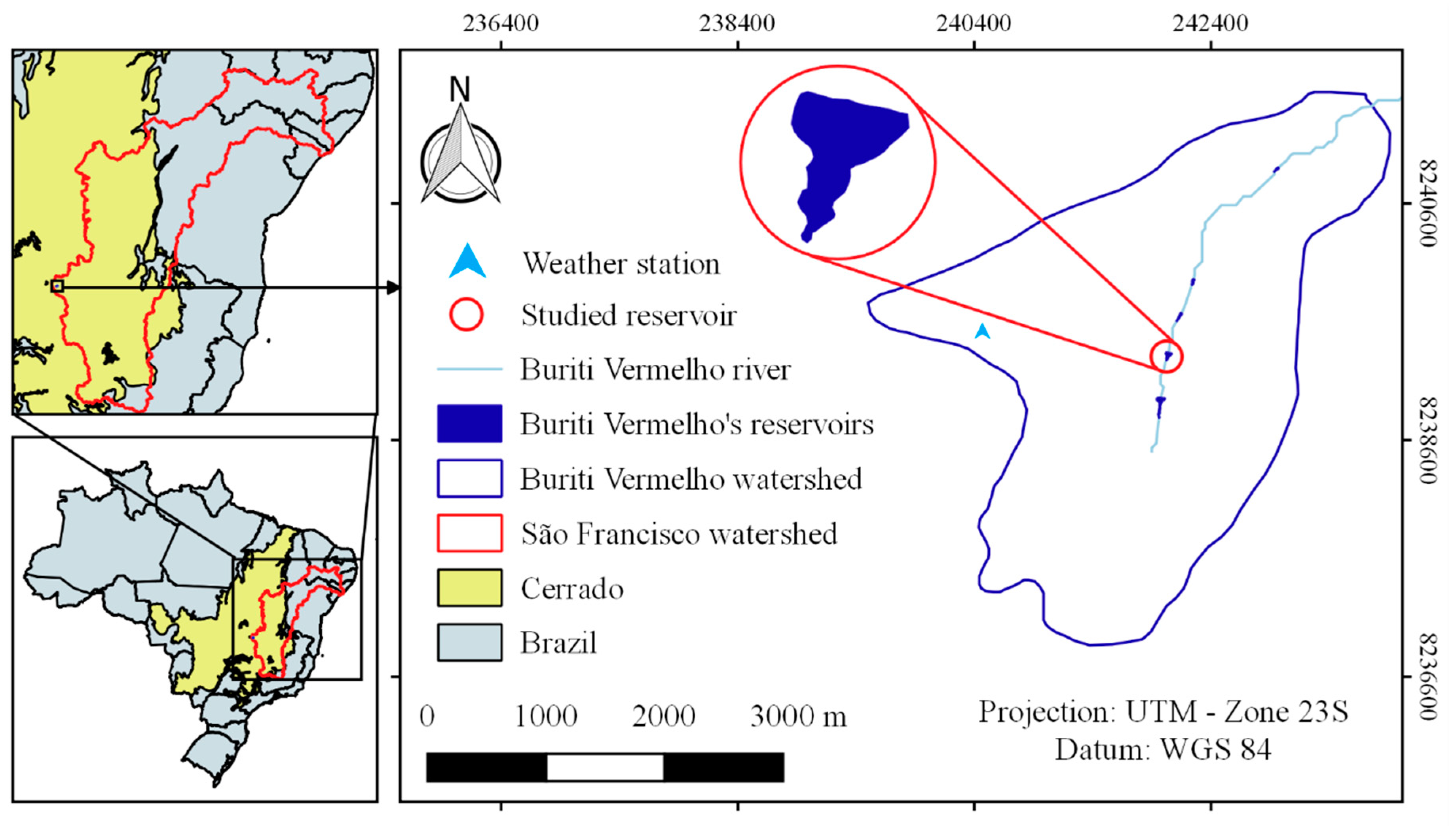
The Buriti Vermelho watershed (Figure 1), with a drainage area of approximately 10 km2, has its main watercourse as a tributary of the right bank of the Estreito River, which, in turn, flows into the Preto River, which is an important sub-basin of the San Francisco watershed. The average annual rainfall of the basin is about 1200 mm, of which 85% corresponds to the rainy season [2].
The small dam used in this study (Figure 1) has 2500 m2 of water surface area and a storage capacity of 3178.7 m3.
2.2. Data
The daily data of temperature, relative humidity, wind speed, and solar radiation were obtained from a meteorological station (EM1) installed near the reservoir (~2 km) for the period from 2010 to 2011. For the same period, the evaporation data were obtained by measurements in a class A pan (TCA) that was installed inside the reservoir. Class A pans are standardized evaporation pans that are made of galvanized or stainless steel, 120.7 cm in diameter, and 25.4 cm deep.
The water level readings in the TCA were performed by a limnigraph (precision = ~0.32 mm) coupled to a datalogger. Whenever the pan water level dropped more than 5 cm, a volume of water that was equivalent to the evaporated water was poured into the pan. The days on which the data collected presented problems, either due to the occurrence of rain or reading failures of the datalogger, were eliminated from the series.
A second meteorological station (EM2), located at ~40 km from the reservoir, was used to obtain a historical series of climatic data (1974 to 2017).
2.3. Methods Used to Estimate Reservoir Evaporation
The methods used (Table 1) vary in complexity and input data, ranging from only requiring maximum and minimum monthly temperature to requiring net radiation, wind speed, and relative humidity.
Although some of the methods that are presented in Table 1 were developed for the calculation of potential evapotranspiration, because the reservoirs present open water surfaces, they can also be used to represent evaporation [1].
The reservoir water temperature, necessary for the energy balance of the water body’s stored heat (Qx), was neglected. Seasonal and interannual temperature changes in the Cerrado region are small, which result in close to no alterations in heat storage [37]. Additionally, many authors have documented heat storage to be insignificant for shallow reservoirs [15,24], and as so it can be disregarded for small ones.
2.4. Performance Analysis of the Employed Equations
The performance of the methods that were applied on a daily basis was also evaluated on a monthly scale. For this, the daily values were accumulated monthly and their average daily evaporations were calculated.
To evaluate the performance of the methods, the Nash-Sutcliffe efficiency index (NSE) [38,39], mean error (MBE), mean absolute error (MAE), and root mean square error (RMSE) were used [40,41].
MBE values averting from zero indicate a tendency to over or underestimate the observed values by the methods. The MAE provides an insight into the general error, while RMSE penalizes errors of higher magnitudes by giving them more weight. In other words, two methods might present the same accuracy, but the RMSE will indicate which is the less precise method [40]. The performance of the method is considered better the closer the MBE, MAE, and RMSE values are to 0.
2.5. Elaboration of Reservoir Evaporation Frequency Curves
An evaporation frequency curve (EC) is a valuable tool for assessing how often a given evaporation will occur. ECs are based on the same principle as flow duration curves [43] and they are used to demonstrate the percentage of time for which evaporation is likely to equal or exceed a given value. Although the EC is sufficient for understanding the distribution of observed or simulated phenomena, its parameterization is fundamental for predicting events and in regionalization studies [44].
In order to elaborate ECs for fortnightly periods, daily evaporation was simulated using historical data from 1974 to 2017 (44 years) and grouped for the desired periods. For example, for the period from 1 to 15 January (Julian days from 1 to 15), 660 data corresponding to daily evaporation values of the first fortnight of the 44 years were used in the EC elaboration.
Evaporation was simulated by the method which, among the evaluated ones, presented the best performance to calculate daily evaporation in small reservoirs in the region. Based on the daily values of each fortnightly period, the evaporation occurrence frequencies were calculated while using Kimball’s Equation [45] (Equation (1)).
where F = frequency (%); m = evaporation event order; and, n = number of observations.
The probability curves were generated from a probability distribution that was derived from the extended Burr XII distribution [44,46] (Equations (2) and (3)).
where λ = scale parameter; α and β = shape parameters; and, t = parameter associated with the percentage of time in which the event is greater than 0.
The parameterization of the equations was performed while using the Levenberg-Marquardt algorithm [47], aimed at the adjustment of non-linear methods by minimizing the sum of the squares of residues.
3. Results
3.1. Evaluation of Observed Data
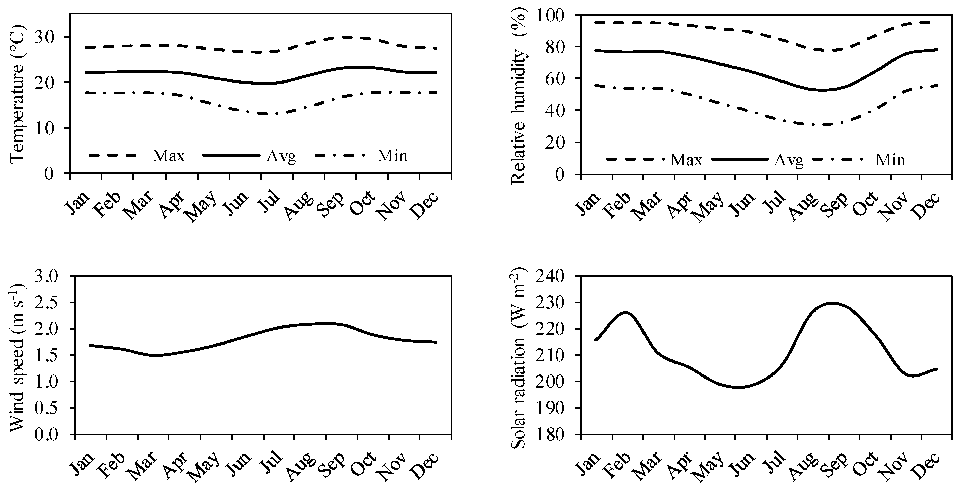
The monthly averages of mean (Ta), maximum (Tx), and minimum (Tn) air temperature, and of mean (RHa), maximum (RHx), and minimum (RHn) relative humidity, wind speed (U2), and solar radiation (Qs) obtained by EM1 (period from 2010 to 2011) and by EM2 (from 1974 to 2017) are shown in Figure 2 and Figure 3, respectively.
The average temperature showed a small variation over the years (Figure 2 and Figure 3), with the monthly average values ranging, for the historical series, between 18.2 °C and 25.4 °C. The maximum temperature values were observed in the months of September and October, while the minimum values were observed in the months of June and July. Analyzing the same figures, it can be seen that the relative humidity decreases from April to August (dry season), with a marked increase in the beginning of the rainy season. The solar radiation recorded the highest values in the months of February, August, and September, and, for the study period, the station near the reservoir presented solar radiation values that were slightly higher than the historical average. The average monthly wind speed, based on historical data, showed its lowest values in the months of February to April, with an average of 1.6 m s−1, and the highest in the months of July to September, with an average of 2.1 m s−1.
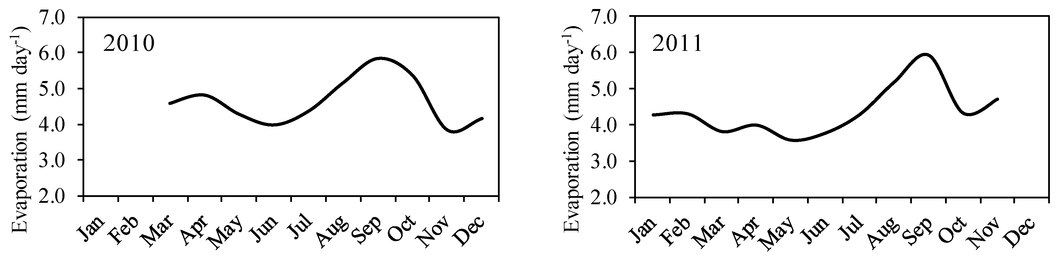
After the elimination of the faults in the series of evaporation data, 312 pairs of data were obtained, where 220 corresponded to the dry season and 92 to the rainy season. It can be observed in Figure 4 that the evaporation had its highest values in September, when the relative humidity was low, and the temperature, wind speed, and radiation were high (Figure 2). The lowest values of evaporation were recorded in the coldest month, June, which also presented low values of radiation.
3.2. Performance of the Methods Used to Estimate Evaporation
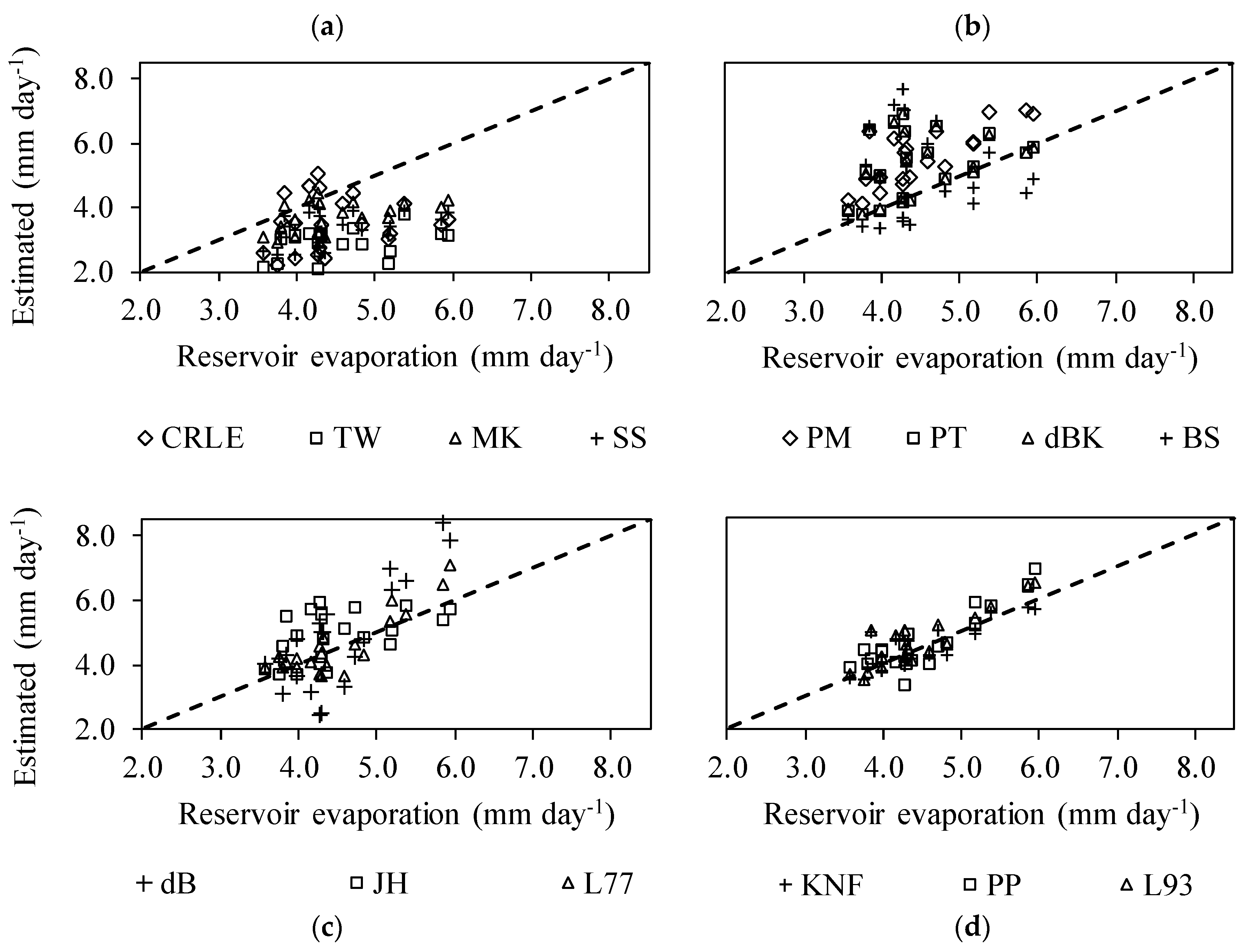
Figure 5 presents monthly average evaporation values that were calculated by different methods. The methods of SS (−0.14 to −2.22 mm) and TW (−0.61 to −2.94 mm) underestimated evaporation in all 21 simulations (Figure 5a). The methods of MK (0.19 to −1.88 mm) and CRLE (0.75 to −2.41 mm) underestimated evaporation values in 86% and 81% of the simulations (Figure 5a), respectively.
The PM method (2.50 to 0.40 mm) (Figure 5b) overestimated the value of evaporation in all of the simulations performed; yet the methods of PT (2.64 to −0.14 mm), dBK (2.63 to −0.15 mm) and BS (3.41 to −1.39 mm) (Figure 5b) overestimated the evaporation value in 71%, 71% and 52% of the simulations, respectively, while the methods of dB (2.57 to −1.84 mm) and L77 (1.16 to −0.92 mm) did so in 62%, and JH (1.69 to −0.61 mm) in 57% (Figure 5c).
Evaporation was better simulated by the PP, L93, and KNF methods (Figure 5d), which presented less dispersion in relation to the 1:1 line. The overestimation of evaporation by the methods of PP (1.02 to −0.88 mm), L93 (1.17 to −0.26 mm) and KNF (1.16 to −0.52 mm) was smaller in magnitude when compared with the other methods and happened in 67%, 62%, and 43% of the simulations, respectively.
The performance criteria of evaporation methods are presented in Table 2 for the time scale for which the methods were developed. The method of PM, for example, was applied on a daily scale, while the PP method was applied on a monthly scale. The performance of the daily methods was also evaluated on a monthly scale.
It can be noted that, both in the daily and monthly scale simulations, only the methods of L93 and KNF had adequate performance (NSE ≥ 0.54), according to the classification of Saleh et al. (2000) [39]. The L93 and KNF methods presented MAE values of 0.56 and 0.54 mm day−1 in the daily scale simulation and 0.44 and 0.38 mm day−1 on the monthly scale, respectively. In the monthly scale simulation, only the method of KNF presented very good performance according to the NSE classification that was presented by Saleh et al. (2000) [39].
In Figure 6, the evaporation values simulated by the methods of KNF and L93 are presented, which were, amongst all of the methods evaluated, the ones with the best performance. The highest monthly evaporation value observed is 7.02 mm day−1, and the smallest is 2.16 mm day−1, both by the method of L93. Outliers appeared more commonly during the dry period, with a tendency to concentrate below the lowest value.
The average monthly evaporation data simulated by the methods, as indicated by the red horizontal line (Figure 6), ranged from 3.56 mm day−1, in May, to 4.99 mm day−1, in September. For the dry season, the L93 method presented the highest average (4.32 mm day−1) and KNF the lowest (4.15 mm day−1), while the opposite happened for the rainy season, where KNF presented the highest average (3.98 mm day−1) and L93 the lowest (3.87 mm day−1).
Figure 7 presents the annual total evaporation values that were simulated by the methods that presented the best performance (KNF and L93) and the trend line of evaporation (1974 to 2017), constructed while taking the average evaporation of the two methods. The gray area between the curves indicates the range of evaporation variation between the two methods.
Trends in evaporation were assessed by a linear model [48,49,50] and their significance by the Student’s t-test [50]. Evaporation exhibited an increasing trend over the years (Figure 7). For the 44 years analyzed, the slope coefficient of the trend line indicated, with a significance of 5% probability by the t-test, a 6.12 mm year−1 increase in the evaporation.
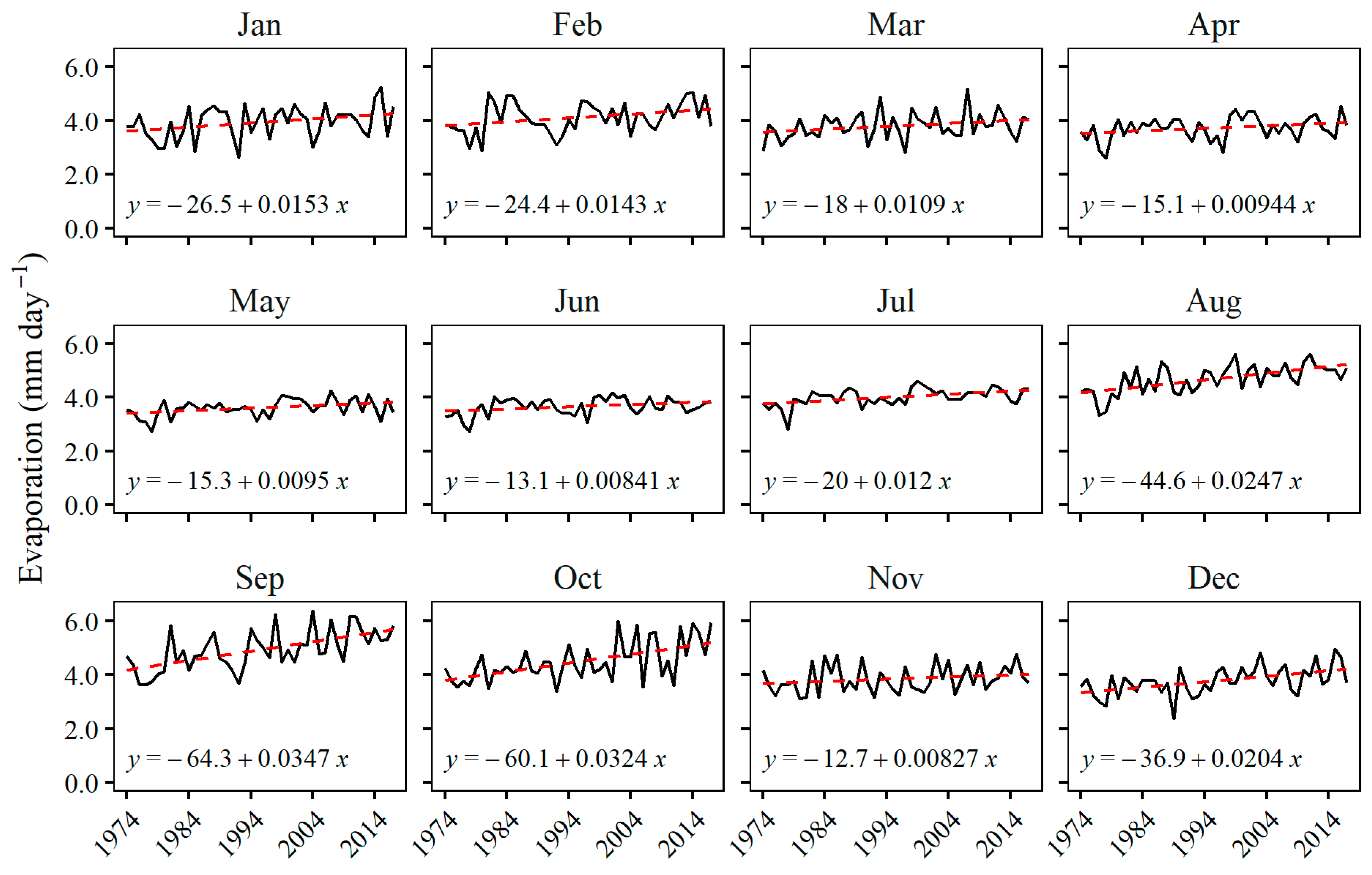
The trend of evaporation variation estimated for the historical series was also evaluated on a monthly basis (Figure 8). Analyzing the trend lines, it was found that all of the angular coefficients of the regressions were significant at 5% probability by the t-test, except for the months of March and April, where the coefficients were significant at 10% probability, and November, which was not significant.
The highest water evaporation values were observed in September (mean = 4.93 mm day−1) and the lowest values in the month of May (mean = 3.61 mm day−1). In general, the lowest variations in the evaporation values were observed during the dry season, with the exception of the months of August and September, a transition period to the rainy season. The lowest monthly values of standard deviation were observed for the months of May, June, and July (0.32 mm), while the highest were observed for the months of September and October (0.73 mm).
It can be seen in Figure 8 that there is an increasing tendency of evaporated water in every month, with angular coefficients that ranged from 0.0083 (November) to 0.0347 mm day−1 year−1 (September). The months that presented the highest monthly evaporation variation by the tendency were September (1.53 mm day−1) and October (1.42 mm day−1), and the months with the lowest significant variation were April (0.42 mm day−1), May (0.42 mm day−1), and June (0.37 mm day−1). For the observed period, the average monthly evaporation increase tendency represented a variation that ranged from 10% in June to 32% in October.
3.3. Reservoir Evaporation Frequency Curves
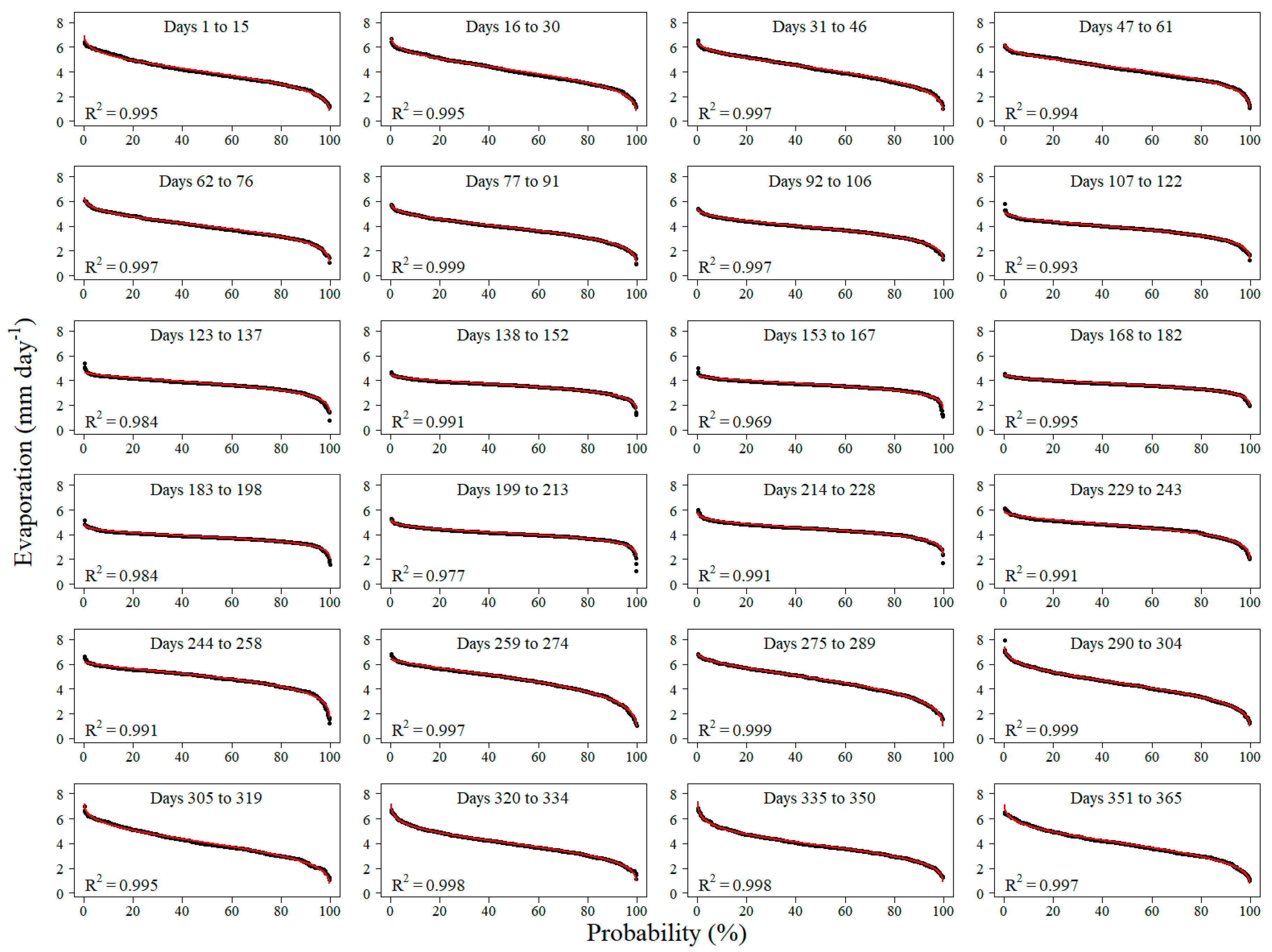
The KNF method presented the best performance among the evaluated methods. For this reason, it was chosen to simulate the evaporation and construct the ECs (Figure 9) based on historical climatic data (44 years). It is noted that the equations presented by Shao et al. (2009) [44] adjusted very well to the ECs, presenting R2 values that ranged from 0.969 to 0.999.
During the dry season, from May to September (Julian days 120 to 272), the EC showed a gentle slope, which indicated that the evaporation value changed very little with the probability. For example, for Julian days varying from 138 to 152 (May 19 to June 2) and for 20% and 80% probability of being matched or exceeded, the reservoir evaporation values varied from 3.95 mm day−1 to 3.11 mm day−1, respectively, with a difference between the values of only 0.84 mm day−1.
During the rainy season (Julian days 1 to 120 and 273 to 365), the EC showed a steeper slope. For example, for Julian days that ranged from 305 to 319 (November 2 to 16) and for 20% and 80% probability of being matched or exceeded, the reservoir evaporation values varied from 5.05 mm day−1 to 2.98 mm day−1, respectively, with a difference between the values of 2.07 mm day−1.
The performance indexes (NSE and RMSE), the evaporation values for the 20% and 60% probability levels and the adjustment parameters (λ, α, and β) of Equations (2) and (3), for each of the fortnightly periods, are presented in Table 3.
The shape parameters α and β are related to the slope and the shape of the upper tail of the EC, respectively. The parameter α varied from 0.094 to 0.271. The higher the value of α, the steeper the EC slope, as can be observed in the Julian days from 259 to 91, representing the months from September to March, where there is greater variability in the evaporation values (Figure 6).
The value of the parameter β ranged from -0.202 to 0.602. The smaller the value of β, the greater the slope of the tail at the top of the curve, the higher its value, and the lower the variation of the values within the low probability range. This behavior can be observed in the Julian days from 335 to 350 (β = −0.202), where the upper part of the EC has a steeper slope when compared, for example, to the period from 259 to 274 (β = 0.602).
The value of λ ranged between 3.802 and 5.627. This parameter relates to the expected evaporation magnitude. The highest values of λ are observed in the periods in which a higher evaporative rate is expected, between Julian days 229 and 289 (August 18 to October 17).
At 20% probability, evaporation in the small dam is predicted to range from 3.95 to 5.68 mm day−1, and at 60% probability, from 3.45 to 4.78 mm day−1. For the same probabilities (20% and 60%), the mean evaporation for the dry season is 4.60 and 3.99 mm day−1, respectively, and for the rainy season is equal to 4.91 and 3.80 mm day−1.
The mean NSE observed for the whole period was equal to 0.993, which indicated a good adjustment of the probability model. The RMSE values ranged from 0.03 to 0.09 mm day−1, with an average of 0.06 mm day−1.
4. Discussion
Potential evaporation had its maximum value when radiation, wind speed, and temperature were high and relative humidity was low, such as in the months from August to October. Even though the beginning of the year might present high radiation and temperature, higher values of relative humidity may strongly limit the potential evaporation, especially in low wind speed conditions, when air moisture accumulates near the air-water interface [51].
Furthermore, the sources of uncertainties in evaporation data collected in pans must be acknowledged. For example, the vapor pressure in the center of reservoirs can be different from the values closer to its shores, which results in microclimate differences between the reservoir and the pan. As a consequence of this, the evaporation measure in the pan can be different from that observed in the reservoir.
Warnaka and Pochop (1988) [52] and Kaya et al. (2016) [14], when comparing class A pans’ observations with evaporation equations, also obtained results in which the method of KNF presented the best performance. In addition, the KNF and L93 methods showed a smaller tendency to underestimate or overestimate the observed values (Table 2). Cabrera et al. (2016) [53] also found good results for the L93 method, where the method performed best (NSE = 0.76) to simulate the daily evaporation of a 20 m2 pan. Although the PM method presented a value of R2 that was close to these two methods, its performance was poor, based on NSE (−0.09) and MBE (0.79 mm day−1).
On the monthly scale, despite the simplicity of the meteorological data required by the PP method, it presented positive NSE and RMSE values that were only slightly higher than the methods of KNF and L93. The PP method was considered by Rosenberry et al. (2007) [1] to be a cost-effective method, since it presented a good performance when compared to several methods of greater complexity. Despite R2 values higher than many methods, the dB and PM methods performed poorly when compared with KNF and L93, for they presented errors with large magnitudes, with a RMSE of the order of 1.22 and 1.23 mm day−1, respectively.
In general, for the monthly evaporation that was simulated for the historical period, the L93 method was the one that presented the greatest dispersion in the simulations, and KNF the smallest. The simulations by both the L93 and KNF methods presented higher dispersion in the months with higher temperature and solar radiation, which are the major variables in the model. A smaller dispersion is observed in cold months due to the nature of the vapor pressure dynamics, which exponentially increases with temperature and it has little difference for lower temperatures.
Based on Figure 7, it is noted that the L93 method, in general, tended to overestimate the evaporation when compared to the KNF method, which can also be observed in Table 2 by the higher MBE values. The average of the two methods’ annual evaporation varied between 1153 and 1671 mm, with a mean equal to 1479 mm. The largest variation (116 mm) between the methods is observed in 1977. For the period from 2002 to 2014, Coelho et al. (2017) [37], evaluating the methods of KNF and L93 to calculate the average annual evaporation of a large reservoir in the Cerrado, obtained values that were equal to 1389 and 1685 mm, respectively, whereas in this work L93 (1484 mm) presented an average only slightly higher than KNF (1474 mm). For Coelho et al. (2017) [37], among the methods used, KNF was the one that presented the lowest values, while the PM and dBK methods presented the highest values.
Additionally, based on Figure 7, the increasing tendency of evaporation over the years is even more relevant when considering that, for the same period, precipitation in the region decreased at a rate of 12 mm year−1. When considering the tendency for growth of evaporation and reduction of precipitation, there is an increasing tendency in the average annual water deficit, by 18.12 mm year−1.
The smaller values of monthly increasing tendency were observed in the beginning of the dry season, when the irrigated crops are highly dependent on stored water. The highest values were observed in the transition period between the dry and rainy seasons, which impacts a key period for the Brazilian savannah’s agriculture. Double cropping viability dramatically increases regional production and it is highly dependent on water supply for early sowing. Climatic changes might escalate the pressure on irrigation reservoirs even further, for they may shorten the wet period and reduce precipitation in the months of September and October [54].
A few important observations were made while investigating the major drivers for the observed tendency increases in evaporation. Daily air mean temperatures were stable during the whole period; maximum air temperature, however, presented an increasing tendency during the entire period. The more significant trends were observed in the months from August to October, which meant that evaporation could present higher peaks along the course of a day. Relative humidity showed a decreasing tendency at the end of the dry season and beginning of the wet season (July to October), which resulted in a higher vapor pressure deficit for the period. Solar and net radiation presented increasing tendencies from August to March, while wind speed presented a small increasing trend for all the months. The months from April to June and November presented reduced tendencies in the meteorological parameters, which resulted in smaller increasing tendencies for evaporation.
Reservoirs are key structures in detecting climate change at the catchment level [55], and their responsiveness is even higher at lower latitudes [9]. Wang et al. (2018) [9] explains that this effect comes from lower latitude lakes and reservoir surface temperatures that require longer periods to warm than air. A water surface at lower temperature results in more long-wave radiation being available for evaporation, which further enhances the process. The temperature of water bodies was not assessed in this study, but water warming as a side effect of climate change can also have many biological and chemical consequences that should be further investigated, such as increased algal and toxic blooms and methane emissions [8].
Observing such increasing trends in evaporation along with unfavorable climate changes is crucial, especially when considering that the impacts of climate change on distributed water availability from small reservoirs are expected to exceed the impacts for large reservoirs [56]. The local social and economic well-being of many regions in the Cerrado strongly relies on water availability from small reservoirs, and their increased evaporation can result in substantial economic loss.
Therefore, investigating which methods perform better in the simulation of small reservoir evaporation is extremely important, especially when these findings give us more confidence in developing tools for a sustainable water resource management, such as evaporation frequency curves (Figure 9, Table 3). Evaporation curves are an important quantitative tool for aiding regional water managers in decision making at desired probabilities and in the planning for higher water availability in small reservoirs. In addition, the curves also provide crucial information for the design of new reservoirs.
5. Conclusions
Indirect methods are an alternative frequently used to overcome the difficulties of direct measurements, and the assessment of such methods for estimating small reservoir evaporation is fundamental while pursuing adequate water resource management. In this work, fourteen methods were assessed to estimate evaporation for small reservoirs in the Brazilian savannah region. The methods that showed the best performance on both daily and monthly time scales were those of Kohler et al. (1955) [21] and Linacre (1993) [24], with Nash-Sutcliffe efficiency indexes of 0.58 and 0.54 on the daily scale, and 0.66 and 0.55 on the monthly scale, respectively.
An increasing tendency of evaporation of approximately 6.12 mm year−1 was observed. The highest monthly increasing tendencies were observed for September and October, which increases the pressure on irrigation reservoirs and jeopardizes local socio-economic development. This raises awareness regarding how significant adequate water management strategies and policies are. Probability curves, which are also presented in this work, are an important quantitative tool for hydrologists and regional water managers, providing crucial information for reservoir operation and the design of new reservoirs.
Estimating small reservoir evaporation with pans comes with many uncertainties, such as the oasis effect, microclimate heterogeneity, and equipment precision. Assessing errors through water balance was not applied in this work, since measurements of water inflow and outflow of the reservoir were not available. The measurement of water infiltration in earth dams also remains a major challenge, which makes the aforementioned implementations promising for future research.
Author Contributions
Conceptualization, D.A. and L.N.R.; writing—original draft preparation, D.A.; writing—review and editing, D.A., L.N.R. and D.D.d.S.
Funding
This research was funded by Coordenação de Aperfeiçoamento de Pessoal de Nível Superior (finance code 001).
Acknowledgments
This study was supported by the Federal District Research Support Foundation (FAP-DF), the Brazilian Agricultural Research Corporation (EMBRAPA Cerrados) and the Federal University of Viçosa (UFV).
Conflicts of Interest
The authors declare no conflict of interest.
References
- Rosenberry, D.O.; Winter, T.C.; Buso, D.C.; Likens, G.E. Comparison of 15 evaporation methods applied to a small mountain lake in the northeastern USA. J. Hydrol. 2007, 340, 149–166. [Google Scholar] [CrossRef]
- Rodrigues, L.N.; Sano, E.E.; Steenhuis, T.S.; Passo, D.P. Estimation of small reservoir storage capacities with remote sensing in the Brazilian Savannah Region. Water Resour. Manag. 2012, 26, 873–882. [Google Scholar] [CrossRef]
- Klink, C.A. Policy intervention in the Cerrado Savannas of Brazil: Changes in the land use and effects on conservation. In Ecology and Conservation of the Maned Wolf: Multidisciplinary Perspectives; Consorte-McCrea, A.G., Ferraz Santos, E., Eds.; CRC Press: Boca Raton, FL, USA, 2014; pp. 293–308. [Google Scholar]
- Brito, L.T.L.; Cavalcanti, N.B.; Silva, A.S.; Pereira, L.A. Produtividade da água de chuva em culturas de subsistência no Semiárido Pernambucano. Eng. Agrícola 2012, 32, 102–109. [Google Scholar] [CrossRef]
- Poussin, J.-C.; Renaudin, L.; Adogoba, D.; Sanon, A.; Tazen, F.; Dogbe, W.; Fusillier, J.-L.; Barbier, B.; Cecchi, P. Performance of small reservoir irrigated schemes in the Upper Volta basin: Case studies in Burkina Faso and Ghana. Water Resour. Rural Dev. 2015, 6, 50–65. [Google Scholar] [CrossRef]
- Rodrigues, L.N.; Ramos, A.E.; Schaedler, H.A.R.; Lopes, A.V.; Figueiredo, G.C. Aspectos legais a serem considerados na construção de pequenas barragens. ITEM Irrig. E Tecnol. Mod. 2008, 80, 53–55. [Google Scholar]
- Friedrich, K.; Grossman, R.L.; Huntington, J.; Blanken, P.D.; Lenters, J.; Holman, K.D.; Gochis, D.; Livneh, B.; Prairie, J.; Skeie, E.; et al. Reservoir evaporation in the Western United States: Current science, challenges, and future needs. Bull. Am. Meteorol. Soc. 2018, 99, 167–187. [Google Scholar] [CrossRef]
- O’Reilly, C.M.; Sharma, S.; Gray, D.K.; Hampton, S.E.; Read, J.S.; Rowley, R.J.; Schneider, P.; Lenters, J.D.; McIntyre, P.B.; Kraemer, B.M.; et al. Rapid and highly variable warming of lake surface waters around the globe. Geophys. Res. Lett. 2015, 42, 10773–10781. [Google Scholar] [CrossRef]
- Wang, W.; Lee, X.; Xiao, W.; Liu, S.; Schultz, N.; Wang, Y.; Zhang, M.; Zhao, L. Global lake evaporation accelerated by changes in surface energy allocation in a warmer climate. Nat. Geosci. 2018, 11, 410–414. [Google Scholar] [CrossRef]
- Kang, M.; Park, S. Modeling water flows in a serial irrigation reservoir system considering irrigation return flows and reservoir operations. Agric. Water Manag. 2014, 143, 131–141. [Google Scholar] [CrossRef]
- Tinoco, V.; Willems, P.; Wyseure, G.; Cisneros, F. Evaluation of reservoir operation strategies for irrigation in the Macul Basin, Ecuador. J. Hydrol. Reg. Stud. 2016, 5, 213–225. [Google Scholar] [CrossRef] [Green Version]
- Lowe, L.D.; Webb, J.A.; Nathan, R.J.; Etchells, T.; Malano, H.M. Evaporation from water supply reservoirs: An assessment of uncertainty. J. Hydrol. 2009, 376, 261–274. [Google Scholar] [CrossRef]
- Wurbs, R.A.; Ayala, R.A. Reservoir evaporation in Texas, USA. J. Hydrol. 2014, 510, 1–9. [Google Scholar] [CrossRef]
- Kaya, S.; Evren, S.; Dașcı, E. Comparison of various equations for estimating class a pan evaporation in semi-arid climate conditions. Ziraat Fakültesi Derg. Uludağ Üniversitesi 2016, 30, 1–9. [Google Scholar]
- Zhao, G.; Gao, H. Estimating reservoir evaporation losses for the United States: Fusing remote sensing and modeling approaches. Remote Sens. Environ. 2019, 226, 109–124. [Google Scholar] [CrossRef] [Green Version]
- Althoff, D.; Rodrigues, L.N.; da Silva, D.D.; Bazame, H.C. Improving methods for estimating small reservoir evaporation in the Brazilian Savanna. Agric. Water Manag. 2019, 216, 105–112. [Google Scholar] [CrossRef]
- Masoner, J.R.; Stannard, D.I.; Christenson, S.C. Differences in evaporation between a floating pan and Class A pan on land. JAWRA J. Am. Water Resour. Assoc. 2008, 44, 552–561. [Google Scholar] [CrossRef]
- Harwell, G.R. Estimation of Evaporation from Open Water: A Review of Selected Studies, Summary of US Army Corps of Engineers Data Collection and Methods, and Evaluation of Two Methods for Estimation of Evaporation from Five Reservoirs in Texas; U.S. Department of the Interior: Washington, DC, USA; U.S. Geological Survey: Reston, VA, USA, 2012.
- Penman, H.L. Natural evaporation from open water, bare soil and grass. Proc. R. Soc. Lond. Ser. A 1948, 193, 120–145. [Google Scholar] [Green Version]
- Antonopoulos, V.Z.; Gianniou, S.K.; Antonopoulos, A.V. Artificial neural networks and empirical equations to estimate daily evaporation: Application to Lake Vegoritis, Greece. Hydrol. Sci. J. 2016, 61, 2590–2599. [Google Scholar] [CrossRef]
- Kohler, M.; Nordenson, T.; Fox, W. Evaporation from Pans and Lakes; US Weather Bureau: Washington, DC, USA, 1955; p. 38.
- Thornthwaite, C.W.; Mather, J.R. The Water Balance; Drexel Institute of Technology, Laboratory of Climatology: Centerton, NJ, USA, 1955; p. 104. [Google Scholar]
- Linacre, E.T. A simple formula for estimating evaporation rates in various climates, using temperature data alone. Agric. Meteorol. 1977, 18, 409–424. [Google Scholar] [CrossRef]
- Linacre, E.T. Data-sparse estimation of lake evaporation, using a simplified Penman equation. Agric. For. Meteorol. 1993, 64, 237–256. [Google Scholar] [CrossRef]
- DeBruin, H.A.R.; Keijman, J.Q. The Priestley-Taylor evaporation model applied to a large, shallow lake in the Netherlands. J. Appl. Meteorol. 1979, 18, 898–903. [Google Scholar] [CrossRef]
- Morton, F.I. Operational estimates of areal evapotranspiration and their significance to the science and practice of hydrology. J. Hydrol. 1983, 66, 1–76. [Google Scholar] [CrossRef]
- Winter, T.C.; Rosenberry, D.O.; Sturrock, A.M. Evaluation of 11 equations for determining evaporation for a small lake in the north central United States. Water Resour. Res. 1995, 31, 983–993. [Google Scholar] [CrossRef]
- Leão, R.A.D.O.; Soares, A.A.; Teixeira, A.D.S.; Silva, D.D.D. Estimation of evaporation in the Banabuiú dam, in the state of Ceará, Brazil, by different combined methods, derived from the Penman equation. Eng. Agrícola 2013, 33, 129–144. [Google Scholar] [CrossRef]
- Stephens, J.C.; Stewart, E.H. A comparison of procedures for computing evaporation and evapotranspiration. Publication 1963, 62, 123–133. [Google Scholar]
- McGuinness, J.L.; Bordne, E.F. A Comparison of Lysimeter-Derived Potential Evapotranspiration with Computed Values; U.S. Department of Agriculture: Washington, DC, USA, 1972.
- Papadakis, J. Potential evapotranspiration. Soil Sci. 1965, 100, 76. [Google Scholar] [CrossRef]
- Thornthwaite, C.W. An approach toward a rational classification of climate. Geogr. Rev. 1948, 38, 55–94. [Google Scholar] [CrossRef]
- Priestley, C.H.B.; Taylor, R.J. On the assessment of surface heat flux and evaporation using large-scale parameters. Mon. Weather Rev. 1972, 100, 81–92. [Google Scholar] [CrossRef]
- DeBruin, H.A.R. A simple model for shallow lake evaporation. J. Appl. Meteorol. 1978, 17, 1132–1134. [Google Scholar] [CrossRef]
- Jensen, M.E.; Haise, H.R. Estimating evapotranspiration from solar radiation. Proc. Am. Soc. Civ. Eng. J. Irrig. Drain. Div. 1963, 89, 15–41. [Google Scholar]
- Brutsaert, W.; Stricker, H. An advection-aridity approach to estimate actual regional evapotranspiration. Water Resour. Res. 1979, 15, 443–450. [Google Scholar] [CrossRef]
- Coelho, C.D.; da Silva, D.D.; Sediyama, G.C.; Moreira, M.C.; Pereira, S.B.; Lana, Â.M.Q. Comparison of the water footprint of two hydropower plants in the Tocantins River Basin of Brazil. J. Clean. Prod. 2017, 153, 164–175. [Google Scholar] [CrossRef]
- Nash, J.E.; Sutcliffe, J.V. River flow forecasting through conceptual models part I—A discussion of principles. J. Hydrol. 1970, 10, 282–290. [Google Scholar] [CrossRef]
- Saleh, A.; Arnold, J.G.; Gassman, P.W.; Hauck, L.M.; Rosenthal, W.D.; Williams, J.R.; McFarland, A.M.S. Application of SWAT for the upper North Bosque River watershed. Trans. ASAE 2000, 43, 1077–1087. [Google Scholar] [CrossRef]
- Willmott, C.J.; Matsuura, K. Advantages of the mean absolute error (MAE) over the root mean square error (RMSE) in assessing average model performance. Clim. Res. 2005, 30, 79–82. [Google Scholar] [CrossRef]
- Richter, K.; Hank, T.B.; Atzberger, C.; Mauser, W. Goodness-of-fit measures: What do they tell about vegetation variable retrieval performance from Earth observation data. In Remote Sensing for Agriculture, Ecosystems, and Hydrology XIII; International Society for Optics and Photonics: Bellingham, WA, USA, 2011; Volume 8174, p. 81740R. [Google Scholar]
- Santhi, C.; Arnold, J.G.; Williams, J.R.; Dugas, W.A.; Srinivasan, R.; Hauck, L.M. Validation of the swat model on a large rwer basin with point and nonpoint sources. J. Am. Water Resour. Assoc. 2001, 37, 1169–1188. [Google Scholar] [CrossRef]
- Searcy, J.K. Flow-Duration Curves; US Government Printing Office: Washington, DC, USA, 1959.
- Shao, Q.; Zhang, L.; Chen, Y.D.; Singh, V.P. A new method for modelling flow duration curves and predicting streamflow regimes under altered land-use conditions. Hydrol. Sci. J. 2009, 54, 606–622. [Google Scholar] [CrossRef]
- Kimball, B.F. On the choice of plotting positions on probability paper. J. Am. Stat. Assoc. 1960, 55, 546–560. [Google Scholar] [CrossRef]
- Shao, Q.; Wong, H.; Xia, J.; Ip, W.-C. Models for extremes using the extended three-parameter Burr XII system with application to flood frequency analysis. Hydrol. Sci. J. 2004, 49, 685–702. [Google Scholar] [CrossRef]
- Moré, J.J. The Levenberg-Marquardt algorithm: Implementation and theory. In Numerical Analysis; Springer: Berlin/Heidelberg, Germany, 1978; pp. 105–116. ISBN 978-3-540-08538-6. [Google Scholar] [Green Version]
- Barnes, E.A.; Barnes, R.J. Estimating linear trends: Simple linear regression versus epoch differences. J. Clim. 2015, 28, 9969–9976. [Google Scholar] [CrossRef]
- Mudelsee, M. Trend analysis of climate time series: A review of methods. Earth Sci. Rev. 2019, 190, 310–322. [Google Scholar] [CrossRef]
- Garfinkel, C.I.; Waugh, D.W.; Polvani, L.M. Recent Hadley cell expansion: The role of internal atmospheric variability in reconciling modeled and observed trends. Geophys. Res. Lett. 2015, 42, 10824–10831. [Google Scholar] [CrossRef]
- Condie, S.A.; Webster, I.T. The influence of wind stress, temperature, and humidity gradients on evaporation from reservoirs. Water Resour. Res. 1997, 33, 2813–2822. [Google Scholar] [CrossRef]
- Warnaka, K.; Pochop, L. Analyses of equations for free water evaporation estimates. Water Resour. Res. 1988, 24, 979–984. [Google Scholar] [CrossRef]
- Cabrera, M.C.; Anache, J.A.A.; Youlton, C.; Wendland, E. Performance of evaporation estimation methods compared with standard 20 m2 tank. Rev. Bras. Eng. Agrícola E Ambient. 2016, 20, 874–879. [Google Scholar] [CrossRef]
- Pires, G.F.; Abrahão, G.M.; Brumatti, L.M.; Oliveira, L.J.; Costa, M.H.; Liddicoat, S.; Kato, E.; Ladle, R.J. Increased climate risk in Brazilian double cropping agriculture systems: Implications for land use in Northern Brazil. Agric. For. Meteorol. 2016, 228, 286–298. [Google Scholar] [CrossRef]
- Adrian, R.; O’Reilly, C.M.; Zagarese, H.; Baines, S.B.; Hessen, D.O.; Keller, W.; Livingstone, D.M.; Sommaruga, R.; Straile, D.; Donk, E.V.; et al. Lakes as sentinels of climate change. Limnol. Oceanogr. 2009, 54, 2283–2297. [Google Scholar] [CrossRef]
- Krol, M.S.; de Vries, M.J.; van Oel, P.R.; de Araújo, J.C. Sustainability of small reservoirs and large scale water availability under current conditions and climate change. Water Resour. Manag. 2011, 25, 3017–3026. [Google Scholar] [CrossRef]
Figure 1.
The Buriti Vermelho watershed, Federal District, Brazil, and the small dam used in the study (red circle).
Figure 1.
The Buriti Vermelho watershed, Federal District, Brazil, and the small dam used in the study (red circle).

Figure 2.
Monthly average climate variables: meteorological station near the reservoir (EM1) for the period from 2010 to 2011.
Figure 2.
Monthly average climate variables: meteorological station near the reservoir (EM1) for the period from 2010 to 2011.

Figure 3.
Monthly average climate variables: meteorological station EM2 for the period from 1974 to 2017.
Figure 3.
Monthly average climate variables: meteorological station EM2 for the period from 1974 to 2017.

Figure 4.
Class A pan evaporation observed for the period from 2010 to 2011.

Figure 5.
Relationship between estimated and observed reservoir evaporation. SS = Stephens and Stewart (1963); MK = Makkink (McGuinness et al. 1972); PP = Papadakis (1965); TW = Thornthwaite (1948); PT = Priestley and Taylor (1972); dB = DeBruin (1978); JH = Jensen and Haise (1963); PM = Penman (1948); BS = Brutsaert and Stricker (1979); dBK = DeBruin and Keijman (1979); CRLE = Morton (1983); L77 = Linacre (1977); L93 = Linacre (1993); KNF = Kohler et al. (1955).

Figure 6.
Monthly average evaporation estimated based on the historical series by the best performing methods—KNF: Kohler et al. (1955) and L93: Linacre (1993). The red line indicates the monthly average simulated.
Figure 6.
Monthly average evaporation estimated based on the historical series by the best performing methods—KNF: Kohler et al. (1955) and L93: Linacre (1993). The red line indicates the monthly average simulated.

Figure 7.
Total annual evaporation estimated by the best performing methods (KNF: Kohler et al. (1955) and L93: Linacre (1993)) based on the historical series and the trend line (dashed line).
Figure 7.
Total annual evaporation estimated by the best performing methods (KNF: Kohler et al. (1955) and L93: Linacre (1993)) based on the historical series and the trend line (dashed line).

Figure 8.
Average monthly evaporation estimated by the average of the best performing methods (KNF: Kohler et al. (1955) and L93: Linacre (1993)) based on the historical series and trend line (dashed line).
Figure 8.
Average monthly evaporation estimated by the average of the best performing methods (KNF: Kohler et al. (1955) and L93: Linacre (1993)) based on the historical series and trend line (dashed line).

Figure 9.
Daily evaporation curves built for fortnightly periods based on the historical climatic data.
Figure 9.
Daily evaporation curves built for fortnightly periods based on the historical climatic data.


Table 1.
Methods used in the estimation of evaporation.
| Methods (Reference) | Equation | Applied |
|---|---|---|
| Stephens and Stewart (1963)—SS [29] | Monthly | |
| Makkink (McGuinness et al. 1972)—MK [30] | Monthly | |
| Papadakis (1965)—PP [31] | Monthly | |
| Thornthwaite (1948)—TW [32] | Monthly | |
| Priestley and Taylor (1972)—PT [33] | >10 days | |
| DeBruin (1978)—dB [34] | >10 days | |
| Jensen and Haise (1963)—JH [35] | >5 days | |
| Penman (1948)—PM [19] | Daily | |
| Brutsaert and Stricker (1979)—BS [36] | Daily | |
| DeBruin and Keijman (1979)—dBK [25] | Daily | |
| Morton (1983)—CRLE [26] | Daily | |
| Linacre (1977)—L77 [23] | Daily | |
| Linacre (1993)—L93 [24] | Daily | |
| Kohler et al. (1955)—KNF [21] | Daily |
E = evaporation (mm day−1); α = 1.26 = empirical constant of Priestley-Taylor; s = slope of the vapor pressure curve (Pa °C−1); γ = psychrometric constant (Pa °C−1); Qn = net radiation (W m−2); Qs = solar radiation (W m−2); Qx = change in heat stored in the water body (W m−2); L = latent heat of vaporization (MJ kg−1); ρ = water density (~1000 kg m−3); I = annual heat index (I = ∑i, i = (Ta/5)1.514); U2 = wind speed at 2 meters from the surface (m s−1); es = vapor saturation pressure at the air temperature (mb); ea = vapor pressure at the air temperature (mb); Ta = mean air temperature (°C) for Thornthwaite and Linacre, and °F for Jensen-Haize and Stephens-Stewart; Td = dew point temperature (°C); d = day number in the month; esmax and esmin = vapor saturation pressure at maximum and minimum temperature (mb); h = altitude (m); Lat = latitude (degrees); P = atmospheric pressure (mb); Ps = atmospheric pressure at sea level (mb); sp = slope of the saturation vapor pressure curve at equilibrium temperature; RTP = net irradiance at equilibrium temperature (W m−2); F = correction factor due to site altitude; Ea = evaporation assuming water temperature is equal to air temperature (mm day−1).
Table 2.
Performance criteria of the evaporation estimation methods.
| Methods | NSE | R2 | RMSE | MAE | MBE |
| Daily Scale | |||||
| KNF | 0.58 | 0.61 | 0.68 | 0.54 | −0.18 |
| L93 | 0.54 | 0.66 | 0.71 | 0.56 | 0.14 |
| L77 | −0.01 | 0.43 | 1.06 | 0.83 | 0.22 |
| PM | −0.09 | 0.54 | 1.10 | 0.89 | 0.79 |
| dBK | −0.19 | 0.19 | 1.15 | 0.85 | 0.26 |
| BS | −1.50 | 0.01 | 1.66 | 1.35 | −0.26 |
| CRLE | −1.91 | 0.15 | 1.79 | 1.59 | −1.44 |
| Methods | NSE | R2 | RMSE | MAE | MBE |
| Monthly Scale | |||||
| KNF | 0.66 | 0.70 | 0.38 | 0.29 | 0.03 |
| L93 | 0.55 | 0.80 | 0.44 | 0.34 | 0.23 |
| PP | 0.43 | 0.75 | 0.49 | 0.42 | 0.19 |
| L77 | 0.41 | 0.76 | 0.50 | 0.40 | 0.09 |
| JH | −0.56 | 0.23 | 0.82 | 0.63 | 0.39 |
| MK | −1.32 | 0.26 | 1.00 | 0.85 | −0.81 |
| dB | −2.46 | 0.64 | 1.22 | 1.04 | 0.33 |
| PM | −2.55 | 0.56 | 1.23 | 1.09 | 1.09 |
| dBK | −2.71 | 0.11 | 1.26 | 0.87 | 0.82 |
| PT | −2.80 | 0.12 | 1.27 | 0.88 | 0.82 |
| SS | −3.25 | 0.23 | 1.35 | 1.21 | −1.21 |
| CRLE | −3.56 | 0.02 | 1.40 | 1.21 | −1.00 |
| BS | −4.77 | 0.01 | 1.57 | 1.26 | 0.56 |
| TW | −6.88 | 0.12 | 1.84 | 1.71 | −1.71 |
NSE = Nash-Sutcliffe efficiency index; R2 = coefficient of determination; RMSE = root mean square error (mm day−1); MAE = mean absolute error (mm day−1); and MBE = mean bias error (mm day−1).
Table 3.
Performance criteria, probable evaporation, and adjusted curve coefficients.
| Interval (Julian days) | Performance Criteria | Evaporation (mm day−1) | Distribution Coefficients | ||||
|---|---|---|---|---|---|---|---|
| NSE | RMSE | 20% * | 60% * | λ | β | α | |
| 1 to 15 | 0.995 | 0.08 | 4.91 | 3.68 | 4.358 | 0.006 | 0.252 |
| 16 to 30 | 0.995 | 0.08 | 5.05 | 3.82 | 4.577 | 0.120 | 0.258 |
| 31 to 46 | 0.997 | 0.06 | 5.13 | 3.93 | 4.766 | 0.252 | 0.261 |
| 47 to 61 | 0.994 | 0.07 | 5.01 | 3.97 | 4.644 | 0.168 | 0.218 |
| 62 to 76 | 0.997 | 0.05 | 4.75 | 3.73 | 4.305 | 0.011 | 0.211 |
| 77 to 91 | 0.999 | 0.03 | 4.55 | 3.61 | 4.186 | 0.110 | 0.213 |
| 92 to 106 | 0.997 | 0.04 | 4.41 | 3.63 | 4.116 | 0.119 | 0.180 |
| 107 to 122 | 0.993 | 0.06 | 4.34 | 3.65 | 4.101 | 0.159 | 0.164 |
| 123 to 137 | 0.984 | 0.08 | 4.18 | 3.59 | 4.045 | 0.351 | 0.156 |
| 138 to 152 | 0.991 | 0.05 | 3.95 | 3.45 | 3.802 | 0.240 | 0.133 |
| 153 to 167 | 0.969 | 0.09 | 3.98 | 3.51 | 3.845 | 0.264 | 0.123 |
| 168 to 182 | 0.995 | 0.03 | 3.98 | 3.55 | 3.814 | 0.086 | 0.102 |
| 183 to 198 | 0.984 | 0.06 | 4.14 | 3.70 | 3.925 | −0.110 | 0.094 |
| 199 to 213 | 0.977 | 0.07 | 4.43 | 3.95 | 4.195 | −0.141 | 0.094 |
| 214 to 228 | 0.991 | 0.05 | 4.85 | 4.30 | 4.573 | −0.151 | 0.099 |
| 229 to 243 | 0.991 | 0.07 | 5.18 | 4.50 | 4.966 | 0.218 | 0.136 |
| 244 to 258 | 0.991 | 0.08 | 5.61 | 4.78 | 5.502 | 0.491 | 0.177 |
| 259 to 274 | 0.997 | 0.06 | 5.67 | 4.53 | 5.627 | 0.602 | 0.264 |
| 275 to 289 | 0.999 | 0.04 | 5.68 | 4.45 | 5.386 | 0.346 | 0.252 |
| 290 to 304 | 0.999 | 0.04 | 5.33 | 4.05 | 4.762 | 0.005 | 0.240 |
| 305 to 319 | 0.995 | 0.08 | 5.05 | 3.73 | 4.482 | 0.040 | 0.271 |
| 320 to 334 | 0.998 | 0.05 | 4.86 | 3.68 | 4.269 | −0.111 | 0.229 |
| 335 to 350 | 0.998 | 0.05 | 4.74 | 3.56 | 4.098 | −0.202 | 0.225 |
| 351 to 365 | 0.997 | 0.07 | 4.93 | 3.64 | 4.348 | −0.001 | 0.263 |
* Probability level; NSE = Nash-Sutcliffe efficiency index; RMSE = root mean squared error (mm day−1).
© 2019 by the authors. Licensee MDPI, Basel, Switzerland. This article is an open access article distributed under the terms and conditions of the Creative Commons Attribution (CC BY) license (http://creativecommons.org/licenses/by/4.0/).
Share and Cite
MDPI and ACS Style
Althoff, D.; Rodrigues, L.N.; da Silva, D.D. Evaluating Evaporation Methods for Estimating Small Reservoir Water Surface Evaporation in the Brazilian Savannah. Water 2019, 11, 1942. https://doi.org/10.3390/w11091942
AMA Style
Althoff D, Rodrigues LN, da Silva DD. Evaluating Evaporation Methods for Estimating Small Reservoir Water Surface Evaporation in the Brazilian Savannah. Water. 2019; 11(9):1942. https://doi.org/10.3390/w11091942
Chicago/Turabian StyleAlthoff, Daniel, Lineu Neiva Rodrigues, and Demetrius David da Silva. 2019. "Evaluating Evaporation Methods for Estimating Small Reservoir Water Surface Evaporation in the Brazilian Savannah" Water 11, no. 9: 1942. https://doi.org/10.3390/w11091942
Note that from the first issue of 2016, this journal uses article numbers instead of page numbers. See further details here.