Seasonal and Scale Effects of Anthropogenic Pressures on Water Quality and Ecological Integrity: A Study in the Sabor River Basin (NE Portugal) Using Partial Least Squares-Path Modeling

 ,
,  ,
,  , and
, and 
Abstract
:1. Introduction
2. Methodology
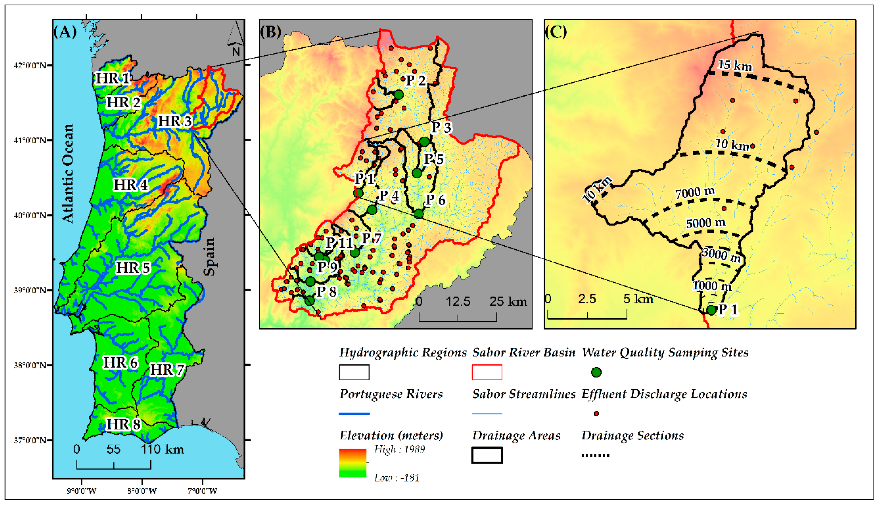
2.1. Study Area
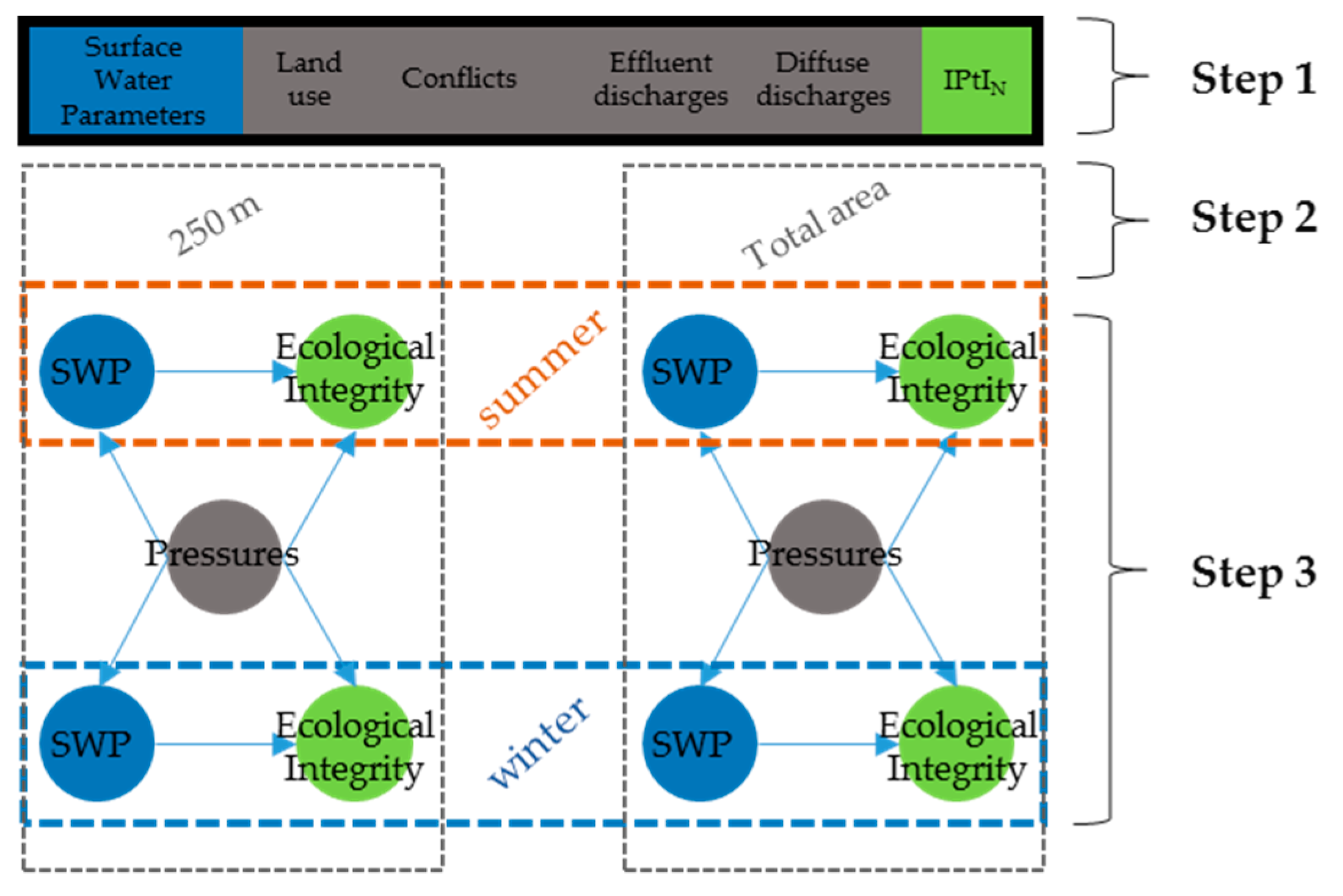
2.2. Materials and Methods
2.3. Dataset Preparation
3. Results
3.1. Spatial Data and Water Quality Parameters
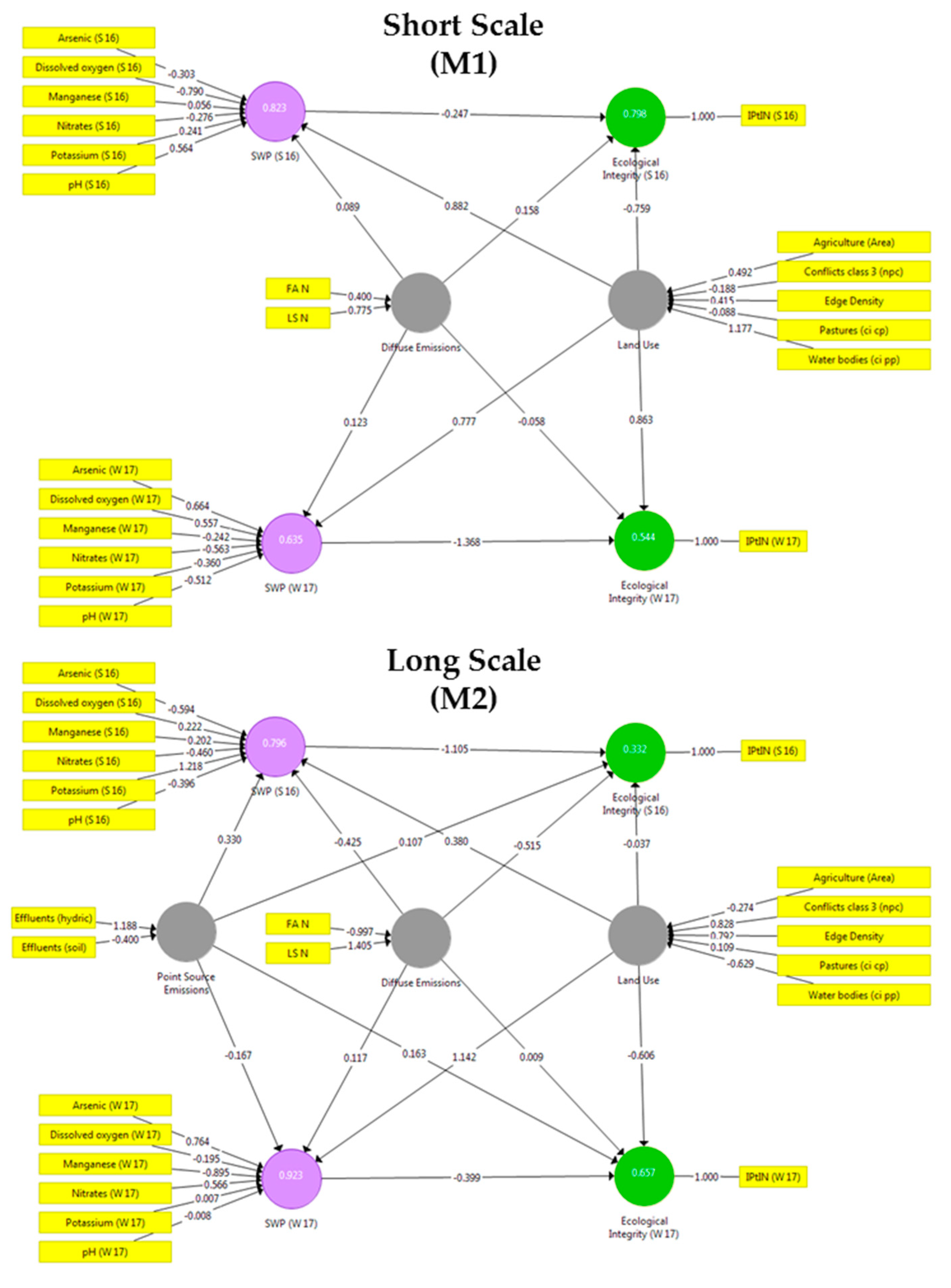
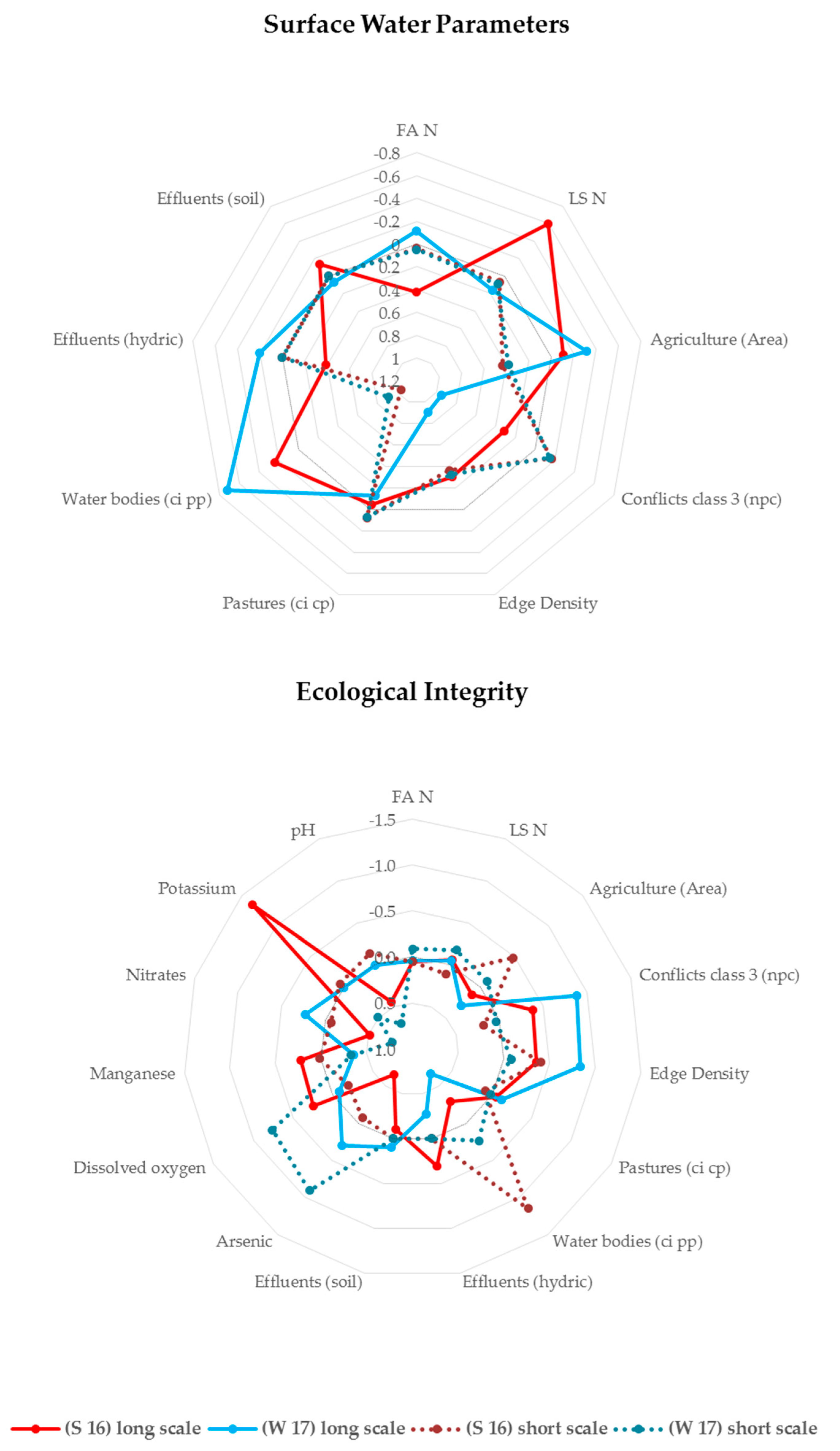
3.2. Results of the Partial Least-Squares Analysis
4. Discussion
4.1. Scope of Study and Environmental Management Guidelines
4.2. Study Limitations and Future Recommendations
5. Conclusions
Author Contributions
Funding
Conflicts of Interest
Appendix A

| Land Use | Agriculture | Pasture | Pasture/Forestry | Forestry | |
|---|---|---|---|---|---|
| Land Capability | |||||
| Agriculture | 0 | 0 | 0 | 0 | |
| Pasture | 1 | 0 | 0 | 0 | |
| Pasture/Forestry | 2 | 1 | 0 | 0 | |
| Forestry | 3 | 2 | 1 | 0 | |
Appendix B
Appendix C
References
- Pacheco, F.; Van Der Weijden, C.H.; Weijden, C.H. Contributions of Water-Rock Interactions to the Composition of Groundwater in Areas with a Sizeable Anthropogenic Input: A Case Study of the Waters of the Fundão Area, Central Portugal. Water Resour. Res. 1996, 32, 3553–3570. [Google Scholar] [CrossRef]
- Pacheco, F.A.L.; Oliveira, A.S.; Van Der Weijden, A.J.; Van Der Weijden, C.H. Weathering, Biomass Production and Groundwater Chemistry in an Area of Dominant Anthropogenic Influence, the Chaves-Vila Pouca de Aguiar Region, North of Portugal. Water Air Soil Pollut. 1999, 115, 481–512. [Google Scholar] [CrossRef]
- Pacheco, F.A.; Van Der Weijden, C.H. Mineral weathering rates calculated from spring water data: A case study in an area with intensive agriculture, the Morais Massif, northeast Portugal. Appl. Geochem. 2002, 17, 583–603. [Google Scholar] [CrossRef]
- Van Der Weijden, C.H.; Pacheco, F.A. Hydrochemistry, weathering and weathering rates on Madeira island. J. Hydrol. 2003, 283, 122–145. [Google Scholar] [CrossRef]
- Van Der Weijden, C.H.; Pacheco, F.A. Hydrogeochemistry in the Vouga River basin (central Portugal): Pollution and chemical weathering. Appl. Geochem. 2006, 21, 580–613. [Google Scholar] [CrossRef]
- Pacheco, F.A.; Szocs, T. “Dedolomitization reactions” driven by anthropogenic activity on loessy sediments, SW Hungary. Appl. Geochem. 2006, 21, 614–631. [Google Scholar] [CrossRef]
- Pacheco, F.A.; Landim, P.M.; Szocs, T. Anthropogenic impacts on mineral weathering: A statistical perspective. Appl. Geochem. 2013, 36, 34–48. [Google Scholar] [CrossRef]
- Santos, R.B.; Fernandes, L.F.S.; Pereira, M.; Cortes, R.; Pacheco, F. Water resources planning for a river basin with recurrent wildfires. Sci. Total Environ. 2015, 526, 1–13. [Google Scholar] [CrossRef]
- Pacheco, F.; Fernandes, L.F.S.; Pacheco, F. Environmental land use conflicts in catchments: A major cause of amplified nitrate in river water. Sci. Total Environ. 2016, 548, 173–188. [Google Scholar] [CrossRef]
- Pacheco, F.A.L.; Santos, R.M.B.; Sanches Fernandes, L.F.; Pereira, M.G.; Cortes, R.M.V. Controls and forecasts of nitrate yields in forested watersheds: A view over mainland Portugal. Sci. Total Environ. 2015, 537, 421–440. [Google Scholar] [CrossRef]
- Santos, R.; Fernandes, L.F.S.; Pereira, M.; Cortes, R.; Pacheco, F. A framework model for investigating the export of phosphorus to surface waters in forested watersheds: Implications to management. Sci. Total Environ. 2015, 536, 295–305. [Google Scholar] [CrossRef] [PubMed]
- Carey, R.O.; Migliaccio, K.W. Contribution of Wastewater Treatment Plant Effluents to Nutrient Dynamics in Aquatic Systems: A Review. Environ. Manag. 2009, 44, 205–217. [Google Scholar] [CrossRef] [PubMed]
- Hayet, C.; Saida, B.A.; Youssef, T.; Hédi, S. Study of biodegradability for municipal and industrial Tunisian wastewater by respirometric technique and batch reactor test. Sustain. Environ. Res. 2016, 26, 55–62. [Google Scholar] [CrossRef] [Green Version]
- Sheoran, A.; Sheoran, V. Heavy metal removal mechanism of acid mine drainage in wetlands: A critical review. Miner. Eng. 2006, 19, 105–116. [Google Scholar] [CrossRef]
- Soares, H.; Boaventura, R.; Machado, A.; Da Silva, J.E.; Da Silva, J.E. Sediments as monitors of heavy metal contamination in the Ave river basin (Portugal): Multivariate analysis of data. Environ. Pollut. 1999, 105, 311–323. [Google Scholar] [CrossRef]
- Serrano-Grijalva, L.; Sánchez-Carrillo, S.; Angeler, D.; Sánchez-Andrés, R.; Álvarez-Cobelas, M. Effects of shrimp-farm effluents on the food web structure in subtropical coastal lagoons. J. Exp. Mar. Biol. Ecol. 2011, 402, 65–74. [Google Scholar] [CrossRef] [Green Version]
- Grizzetti, B.; Bouraoui, F.; De Marsily, G. Assessing nitrogen pressures on European surface water. Glob. Biogeochem. Cycles 2008, 22, GB4023. [Google Scholar] [CrossRef]
- Moss, B. Water pollution by agriculture. Philos. Trans. R. Soc. B Biol. Sci. 2008, 363, 659–666. [Google Scholar] [CrossRef]
- Ayers, R.S.; Westcot, D.W. Water Quality for Agriculture; FAO United Nations: Rome, Italy, 1985. [Google Scholar]
- Ali, H.; Khan, E.; Sajad, M.A. Phytoremediation of heavy metals—Concepts and applications. Chemosphere 2013, 91, 869–881. [Google Scholar] [CrossRef]
- Sheng, Y.; Qu, Y.; Ding, C.; Sun, Q.; Mortimer, R.J. A combined application of different engineering and biological techniques to remediate a heavily polluted river. Ecol. Eng. 2013, 57, 1–7. [Google Scholar] [CrossRef]
- Palmer, M.; Bernhardt, E.; Allan, J.D.; Lake, P.; Alexander, G.; Brooks, S.; Carr, J.; Clayton, S.; Dahm, C.N.; Shah, J.F.; et al. Standards for ecologically successful river restoration. J. Appl. Ecol. 2005, 42, 208–217. [Google Scholar] [CrossRef]
- Groffman, P.M.; Bain, D.J.; Band, L.E.; Belt, K.T.; Brush, G.S.; Grove, J.M.; Pouyat, R.V.; Yesilonis, I.C.; Zipperer, W.C. Down by the riverside: Urban riparian ecology. Front. Ecol. Environ. 2003, 1, 315–321. [Google Scholar] [CrossRef]
- Nilsson, C.; Svedmark, M. Basic Principles and Ecological Consequences of Changing Water Regimes: Riparian Plant Communities. Environ. Manag. 2002, 30, 468–480. [Google Scholar] [CrossRef]
- Fernandes, M.R.; Aguiar, F.C.; Ferreira, M.T.; Fernandes, M.R. Assessing riparian vegetation structure and the influence of land use using landscape metrics and geostatistical tools. Landsc. Urban Plan. 2011, 99, 166–177. [Google Scholar] [CrossRef] [Green Version]
- McGarigal, K.; Marks, B.J. FRAGSTATS: Spatial Pattern Analysis Program for Quantifying Landscape Structure; US Forest Service Pacific Northwest Research Station: Corvallis, OR, USA, 1995; p. 351.
- Adamczyk, J.; Tiede, D. ZonalMetrics—A Python toolbox for zonal landscape structure analysis. Comput. Geosci. 2017, 99, 91–99. [Google Scholar] [CrossRef]
- Johnson, L.; Richards, C.; Host, G.; Arthur, J. Landscape influences on water chemistry in Midwestern stream ecosystems. Freshw. Biol. 1997, 37, 193–208. [Google Scholar] [CrossRef]
- Łowicki, D. Prediction of flowing water pollution on the basis of landscape metrics as a tool supporting delimitation of Nitrate Vulnerable Zones. Ecol. Indic. 2012, 23, 27–33. [Google Scholar] [CrossRef]
- Uuemaa, E.; Roosaare, J.; Mander, U. Scale dependence of landscape metrics and their indicatory value for nutrient and organic matter losses from catchments. Ecol. Indic. 2005, 5, 350–369. [Google Scholar] [CrossRef]
- Lee, S.W.; Hwang, S.J.; Lee, S.B.; Hwang, H.S.; Sung, H.C. Landscape ecological approach to the relationships of land use patterns in watersheds to water quality characteristics. Landsc. Urban Plan. 2009, 92, 80–89. [Google Scholar] [CrossRef]
- Ding, J.; Jiang, Y.; Liu, Q.; Hou, Z.; Liao, J.; Fu, L.; Peng, Q. Influences of the land use pattern on water quality in low-order streams of the Dongjiang River basin, China: A multi-scale analysis. Sci. Total Environ. 2016, 551, 205–216. [Google Scholar] [CrossRef]
- Morley, S.A.; Karr, J.R. Assessing and Restoring the Health of Urban Streams in the Puget Sound Basin. Conserv. Biol. 2002, 16, 1498–1509. [Google Scholar] [CrossRef] [Green Version]
- Allan, D.; Erickson, D.; Fay, J. The influence of catchment land use on stream integrity across multiple spatial scales. Freshw. Biol. 1997, 37, 149–161. [Google Scholar] [CrossRef] [Green Version]
- Zhang, J.; Li, S.; Dong, R.; Jiang, C.; Ni, M. Influences of land use metrics at multi-spatial scales on seasonal water quality: A case study of river systems in the Three Gorges Reservoir Area, China. J. Clean. Prod. 2019, 206, 76–85. [Google Scholar] [CrossRef]
- Dodds, W.K.; Oakes, R.M. Headwater influences on downstream water quality. Environ. Manag. 2008, 41, 367–377. [Google Scholar] [CrossRef] [PubMed]
- Schiff, R.; Benoit, G. Effects of Impervious Cover at Multiple Spatial Scales on Coastal Watershed Streams. JAWRA J. Am. Water Resour. Assoc. 2007, 43, 712–730. [Google Scholar] [CrossRef]
- Yu, S.; Xu, Z.; Wu, W.; Zuo, D. Effect of land use types on stream water quality under seasonal variation and topographic characteristics in the Wei River basin, China. Ecol. Indic. 2016, 60, 202–212. [Google Scholar] [CrossRef]
- Junior, R.V.; Galbiatti, J.; Pissarra, T.; Filho, M.M. Diagnóstico do Conflito de Uso e Ocupação do Solo na Bacia do Rio Uberaba. Glob. Sci. Technol. 2013, 6, 40–52. [Google Scholar] [CrossRef]
- Valera, C.; Junior, R.F.V.; Varandas, S.; Fernandes, L.S.; Pacheco, F.; Fernandes, L.F.S.; Pacheco, F. The role of environmental land use conflicts in soil fertility: A study on the Uberaba River basin, Brazil. Sci. Total Environ. 2016, 562, 463–473. [Google Scholar] [CrossRef]
- Valera, C.A.; Pissarra, T.C.T.; Martins Filho, M.V.; Valle Junior, R.F.; Sanches Fernandes, L.F.; Pacheco, F.A.L. A legal framework with scientific basis for applying the ‘polluter pays principle’ to soil conservation in rural watersheds in Brazil. Land Use Policy 2017, 66, 61–71. [Google Scholar] [CrossRef]
- Caldas, A.; Pissarra, T.; Costa, R.; Neto, F.; Zanata, M.; Parahyba, R.; Sanches Fernandes, L.; Pacheco, F.; Caldas, A.M.; Pissarra, T.C.T.; et al. Flood Vulnerability, Environmental Land Use Conflicts, and Conservation of Soil and Water: A Study in the Batatais SP Municipality, Brazil. Water 2018, 10, 1357. [Google Scholar] [CrossRef]
- Junior, R.V.; Varandas, S.; Fernandes, L.S.; Pacheco, F.; Junior, R.F.V.; Fernandes, L.F.S.; Pacheco, F. Environmental land use conflicts: A threat to soil conservation. Land Use Policy 2014, 41, 172–185. [Google Scholar] [CrossRef]
- Pacheco, F.; Varandas, S.; Fernandes, L.S.; Junior, R.V.; Pacheco, F.; Fernandes, L.F.S.; Junior, R.F.V. Soil losses in rural watersheds with environmental land use conflicts. Sci. Total Environ. 2014, 485, 110–120. [Google Scholar] [CrossRef] [PubMed]
- Junior, R.V.; Varandas, S.; Fernandes, L.S.; Pacheco, F.; Junior, R.F.V.; Fernandes, L.F.S.; Pacheco, F. Multi Criteria Analysis for the monitoring of aquifer vulnerability: A scientific tool in environmental policy. Environ. Sci. Policy 2015, 48, 250–264. [Google Scholar] [CrossRef] [Green Version]
- Valle, R.; Varandas, S.; Fernandes, L.S.; Pacheco, F.; Fernandes, L.F.S.; Pacheco, F. Groundwater quality in rural watersheds with environmental land use conflicts. Sci. Total Environ. 2014, 493, 812–827. [Google Scholar] [CrossRef] [PubMed]
- Bellu, A.; Fernandes, L.F.S.; Cortes, R.M.; Pacheco, F.A.; Fernandes, L.F.S. A framework model for the dimensioning and allocation of a detention basin system: The case of a flood-prone mountainous watershed. J. Hydrol. 2016, 533, 567–580. [Google Scholar] [CrossRef]
- Junior, R.F.V.; Varandas, S.G.; Pacheco, F.A.; Pereira, V.R.; Santos, C.F.; Cortes, R.M.; Fernandes, L.F.S.; Junior, R.F.V.; Fernandes, L.F.S. Impacts of land use conflicts on riverine ecosystems. Land Use Policy 2015, 43, 48–62. [Google Scholar] [CrossRef]
- Fonseca, A.; Fernandes, L.S.; Fontainhas-Fernandes, A.; Monteiro, S.M.; Pacheco, F.; Fernandes, L.F.S.; Pacheco, F. From catchment to fish: Impact of anthropogenic pressures on gill histopathology. Sci. Total Environ. 2016, 550, 972–986. [Google Scholar] [CrossRef] [PubMed]
- Fonseca, A.; Fernandes, L.S.; Fontainhas-Fernandes, A.; Monteiro, S.M.; Pacheco, F.; Fernandes, L.F.S.; Pacheco, F. The impact of freshwater metal concentrations on the severity of histopathological changes in fish gills: A statistical perspective. Sci. Total Environ. 2017, 599, 217–226. [Google Scholar] [CrossRef]
- Oliveira, S.V.; Cortes, R. Environmental indicators of ecological integrity and their development for running waters in northern Portugal. Limnetica 2006, 25, 479–498. [Google Scholar]
- Carignan, V.; Villard, M.-A. Selecting Indicator Species to Monitor Ecological Integrity: A Review. Environ. Monit. Assess. 2002, 78, 45–61. [Google Scholar] [CrossRef]
- Alba-Tercedor, J.; Jaímez-Cuéllar, P.; Aĺvarez, M.; Avileś, J.; Bonada, N.; Casas, J.; Mellado, A.; Ortega, M.; Pardo, I.; Prat, N.; et al. Caracterización del estado ecológico de ríos mediterráneos ibéricos mediante el índice IBMWP (antes BMWP’). Limnetica 2002, 21, 175–185. [Google Scholar]
- INAG. Critérios Para a Classificação do Estado das Massas de Água Superficiais–Rios e Albufeiras; Technical Report; Instituto da Água I.P.: Lisbon, Portugal, 2009; 71p, Available online: https://apambiente.pt/dqa/assets/crit%C3%A9rios-classifica%C3%A7%C3%A3o-rios-e-albufeiras.pdf (accessed on 15 February 2019).
- Cortes, R.; Hughes, S.; Coimbra, A.; Monteiro, S.M.; Pereira, V.; Lopes, M.; Pereira, S.; Pinto, A.; Sampaio, A.; Santos, C.; et al. A multiple index integrating different levels of organization. Ecotoxicol. Environ. Saf. 2016, 132, 270–278. [Google Scholar] [CrossRef] [PubMed]
- Pacheco, F.A.L. Application of Correspondence Analysis in the Assessment of Groundwater Chemistry. Math. Geol. 1998, 30, 129–161. [Google Scholar] [CrossRef]
- Pacheco, F.A.L.; Landin, P.M.B. Two-way regionalized classification of multivariate datasets and its application to the assessment of hydrodynamic dispersion. Math. Geol. 2005, 37, 393–417. [Google Scholar] [CrossRef]
- Astrachan, C.B.; Patel, V.K.; Wanzenried, G. A comparative study of CB-SEM and PLS-SEM for theory development in family firm research. J. Fam. Bus. Strat. 2014, 5, 116–128. [Google Scholar] [CrossRef]
- Hair, J.F.; Hult, G.T.M.; Ringle, C.; Sarstedt, M. A Primer on Partial Least Squares Structural Equation Modeling; Sage Publishing Inc.: Thousand Oaks, CA, USA, 2014. [Google Scholar]
- Zou, S.; Yu, Y.-S. A general structural equation model for river water quality data. J. Hydrol. 1994, 162, 197–209. [Google Scholar] [CrossRef]
- Chenini, I.; Khemiri, S. Evaluation of ground water quality using multiple linear regression and structural equation modeling. Int. J. Environ. Sci. Technol. 2009, 6, 509–519. [Google Scholar] [CrossRef] [Green Version]
- Wu, E.M.Y.; Tsai, C.C.; Cheng, J.F.; Kuo, S.L.; Lu, W.T. The Application of Water Quality Monitoring Data in a Reservoir Watershed Using AMOS Confirmatory Factor Analyses. Environ. Model. Assess. 2014, 19, 325–333. [Google Scholar] [CrossRef]
- Levêque, J.G.; Burns, R.C. A Structural Equation Modeling approach to water quality perceptions. J. Environ. Manag. 2017, 197, 440–447. [Google Scholar] [CrossRef] [Green Version]
- Fernandes, L.S.; Fernandes, A.; Ferreira, A.; Cortes, R.; Pacheco, F. A partial least squares—Path modeling analysis for the understanding of biodiversity loss in rural and urban watersheds in Portugal. Sci. Total Environ. 2018, 626, 1069–1085. [Google Scholar] [CrossRef]
- Terêncio, D.; Fernandes, L.S.; Cortes, R.; Moura, J.; Pacheco, F.; Pacheco, F. Rainwater harvesting in catchments for agro-forestry uses: A study focused on the balance between sustainability values and storage capacity. Sci. Total Environ. 2018, 613, 1079–1092. [Google Scholar] [CrossRef] [PubMed]
- APA. ARHNorte Relatório de Base—Parte 2 (Caracterização e Diagnóstico da Região Hidrográfica); APA: Washington, DC, USA, 2012. [Google Scholar]
- DGTerritório. The 2015 Map of Land Uses in Portugal (Carta de Uso e Ocupação do Solo in Portuguese). Available online: http://www.dgterritorio.pt/dados_abertos/cos/ (accessed on 18 February 2019).
- Santos, R.; Fernandes, L.S.; Cortes, R.; Pacheco, F. Analysis of hydrology and water allocation with swat and mike hydro basin in the sabor river basin, portugal. Environ. Impact IV 2018, 215, 347–355. [Google Scholar]
- Pereira, M.G.; Malamud, B.D.; Trigo, R.M.; Alves, P.I.; Trigo, R. The history and characteristics of the 1980–2005 Portuguese rural fire database. Nat. Hazards Earth Syst. Sci. 2011, 11, 3343–3358. [Google Scholar] [CrossRef]
- Gonçalves, D. Contribuição Para o Estudo Do Clima da Bacia Superior do Rio Sabor. Influência da Circulação Geral e Regional na Estrutura de Baixa Atmosfera; Universidade de Trás-os-Montes e Alto Douro: Vila Real, Portugal, 1985; 510p. [Google Scholar]
- Santos, R.; Fernandes, L.S.; Cortes, R.; Varandas, S.; Jesus, J.; Pacheco, F.; Fernandes, L.F.S.; Pacheco, F. Integrative assessment of river damming impacts on aquatic fauna in a Portuguese reservoir. Sci. Total Environ. 2017, 601, 1108–1118. [Google Scholar] [CrossRef] [PubMed]
- PGRH2 - Plano de Gestão da Região Hidrográfica do Cávado Parte 2, Ave e Leça (RH2); Technical Report; Administração da Região Hidrográfica do Norte, I.P.: Lisbon, Portugal, 2016; 193p. (In Portuguese)
- Agência Portuguesa do Ambiente. Available online: https://www.apambiente.pt/ (accessed on 23 July 2019).
- EEA Data and Maps—European Environment Agency. Available online: https://www.eea.europa.eu/data-and-maps (accessed on 12 December 2018).
- ESRI. ArcMap version 10.1. Environ. Syst. Resour. Inst. 2012. Available online: http://desktop.arcgis.com/en/arcmap/ (accessed on 18 September 2019).
- Pacheco, F.A.; Alencoão, A.M. Role of fractures in weathering of solid rocks: Narrowing the gap between laboratory and field weathering rates. J. Hydrol. 2006, 316, 248–265. [Google Scholar] [CrossRef]
- Pacheco, F.A.; Van Der Weijden, C.H. Role of hydraulic diffusivity in the decrease of weathering rates over time. J. Hydrol. 2014, 512, 87–106. [Google Scholar] [CrossRef]
- Pacheco, F.A.; Van Der Weijden, C.H. Weathering of plagioclase across variable flow and solute transport regimes. J. Hydrol. 2012, 420, 46–58. [Google Scholar] [CrossRef]
- Terêncio, D.; Fernandes, L.S.; Cortes, R.; Pacheco, F.; Fernandes, L.F.S.; Pacheco, F. Improved framework model to allocate optimal rainwater harvesting sites in small watersheds for agro-forestry uses. J. Hydrol. 2017, 550, 318–330. [Google Scholar] [CrossRef]
- Fernandes, L.F.S.; Dos Santos, C.M.M.; Pereira, A.P.; Moura, J.P. Model of management and decision support systems in the distribution of water for consumption: Case study in North Portugal. Eur. J. Environ. Civ. Eng. 2011, 15, 411–426. [Google Scholar] [CrossRef]
- Pinto, A.A.S.; Fernandes, L.F.S.; De Oliveira Maia, R.J.F. A method for selecting suitable technical solutions to support sustainable riverbank stabilisation. Area 2018, 51, 285–298. [Google Scholar] [CrossRef]
- Fernandes, L.F.S.; Marques, M.J.; Oliveira, P.C.; Moura, J.P. Decision support systems in water resources in the demarcated region of Douro—Case study in Pinhão river basin, Portugal. Water Environ. J. 2014, 28, 350–357. [Google Scholar] [CrossRef]
- ESRI. ArcHydro Tools for ArcGIS 10. Environ. Syst. Resour. Inst. 2012. Available online: http://downloads.esri.com/ArcHydro/ArcHydro/Setup/10.1/ (accessed on 18 September 2019).
- EC—European Commission. Common Implementation Strategy for the Water Framework Directive (2000/60/EC); Guidance document no. 19, guidance on surface water chemical monitoring under the water framework directive. Technical Report - 2009–025; Office for Official Publications of the European Communities: Luxembourg, 2009; 132p. [Google Scholar]
- EC—European Commission. Common Implementation Strategy for the Water Framework Directive (2000/60/EC); Guidance document no. 7—Monitoring under the Water Framework Directive. Technical Report; Office for Official Publications of the European Communities: Luxembourg, 2003; 160p. [Google Scholar]
- Monecke, A.; Leisch, F. semPLS: Structural Equation Modeling Using Partial Least Squares. J. Stat. Softw. 2012, 48, 1–32. [Google Scholar] [CrossRef] [Green Version]
- Ringle, C.M.; Wende, S.; Will, A. Smart PLS. 2015. Available online: https://www.smartpls.com/ (accessed on 15 February 2019).
- Fernandes, A.; Ferreira, A.; Fernandes, L.S.; Cortes, R.; Pacheco, F. Path modelling analysis of pollution sources and environmental consequences in river basins. WIT Trans. Ecol. Environ. 2018, 228, 79–87. [Google Scholar]
- Salgado Terêncio, D.P.; Sanches Fernandes, L.F.; Vitor Cortes, R.M.; Moura, J.P.; Leal Pacheco, F.A.; Salgado Terêncio, D.P.; Sanches Fernandes, L.F.; Vitor Cortes, R.M.; Moura, J.P.; Leal Pacheco, F.A. Can Land Cover Changes Mitigate Large Floods? A Reflection Based on Partial Least Squares-Path Modeling. Water 2019, 11, 1464. [Google Scholar] [CrossRef]
- Decree-Law No. 236/98. Diário da República No. 176/1998. Série I-A de 1998-08-01. 1998, pp. 3676–3722. Available online: https://data.dre.pt/eli/dec-lei/236/1998/08/01/p/dre/pt/html (accessed on 20 March 2019).
- Ravenscroft, P.; Brammer, H.; Richards, K. Arsenic Pollution: A Global Synthesis; Wiley-Blackwell: Hoboken, NJ, USA, 2009; 618p, ISBN 9781405186025. [Google Scholar]
- Jayasumana, C.; Fonseka, S.; Fernando, A.; Jayalath, K.; Amarasinghe, M.; Siribaddana, S.; Gunatilake, S.; Paranagama, P. Phosphate fertilizer is a main source of arsenic in areas affected with chronic kidney disease of unknown etiology in Sri Lanka. SpringerPlus 2015, 4, 90. [Google Scholar] [CrossRef] [PubMed]
- Jayasumana, C.; Fonseka, S.; Fernando, A.; Jayalth, K.; Amarasinghe, M.; Paranagma, P. Presence of arsenic in agrochemicals and their association with the agricultural chronic kidney disease in Sri Lanka. J. Toxicol. Health 2014, Photon 104, 352–361. [Google Scholar]
- Suriyagoda, L.D.; Dittert, K.; Lambers, H. Arsenic in Rice Soils and Potential Agronomic Mitigation Strategies to Reduce Arsenic Bioavailability: A Review. Pedosphere 2018, 28, 363–382. [Google Scholar] [CrossRef]
- Bhattacharya, P.; Welch, A.H.; Stollenwerk, K.G.; McLaughlin, M.J.; Bundschuh, J.; Panaullah, G. Arsenic in the environment: Biology and Chemistry. Sci. Total Environ. 2007, 379, 109–120. [Google Scholar] [CrossRef]
- Canivet, P.C.V.; Canivet, V.; Chambon, P.; Gibert, J. Toxicity and Bioaccumulation of Arsenic and Chromium in Epigean and Hypogean Freshwater Macroinvertebrates. Arch. Environ. Contam. Toxicol. 2001, 40, 345–354. [Google Scholar] [CrossRef] [PubMed]
- Römheld, V.; Kirkby, E.A. Research on potassium in agriculture: Needs and prospects. Plant Soil 2010, 335, 155–180. [Google Scholar] [CrossRef]
- Mpelasoka, B.S.; Schachtman, D.P.; Treeby, M.T.; Thomas, M.R. A review of potassium nutrition in grapevines with special emphasis on berry accumulation. Aust. J. Grape Wine Res. 2003, 9, 154–168. [Google Scholar] [CrossRef]
- Dag, A.; Kerem, Z.; Erel, R.; Basheer, L.; Yermiyahu, U.; Ben-Gal, A.; Ben-David, E. Olive oil composition as a function of nitrogen, phosphorus and potassium plant nutrition. J. Sci. Food Agric. 2009, 89, 1871–1878. [Google Scholar] [CrossRef]
- Jones, J.P.; Sudicky, E.A.; Brookfield, A.; Park, Y.-J. An assessment of the tracer-based approach to quantifying groundwater contributions to streamflow. Water Resour. Res. 2006, 42, W02407. [Google Scholar] [CrossRef]
- Uuemaa, E.; Roosaare, J.; Mander, Ü. Landscape metrics as indicators of river water quality at catchment scale. Hydrol. Res. 2007, 38, 125–138. [Google Scholar] [CrossRef]
- Wiens, J.A. Riverine landscapes: Taking landscape ecology into the water. Freshw. Biol. 2002, 47, 501–515. [Google Scholar] [CrossRef]
- Ferreira, A.; Fernandes, L.S.; Cortes, R.; Pacheco, F.; Fernandes, L.F.S.; Pacheco, F. Assessing anthropogenic impacts on riverine ecosystems using nested partial least squares regression. Sci. Total Environ. 2017, 583, 466–477. [Google Scholar] [CrossRef]
- DGADR—Direção-Geral de Agricultura e Desenvolvimento Rural. Available online: https://www.dgadr.gov.pt/ (accessed on 23 February 2019).
- Sharpley, A. Managing agricultural phosphorus to minimize water quality impacts. Sci. Agric. 2015, 73, 1–8. [Google Scholar] [CrossRef]
- Hooda, P.; Edwards, A.; Anderson, H.; Miller, A. A review of water quality concerns in livestock farming areas. Sci. Total Environ. 2000, 250, 143–167. [Google Scholar] [CrossRef]
- Peden, D.; Tadesse, G.; Misra, A.K.; Ahmed, F.A.; Astatke, A.; Ayalneh, W.; Herrero, M.; Kiwuwa, G.; Kumsa, T.; Mati, B.; et al. Water and Livestock for Human development. In Water for Food Water for Life: A Comprehensive Assessment of Water Management in Agriculture; Springer: Berlin/Heidelberg, Germany, 2013; ISBN 9781849773799. [Google Scholar]
- Sahoo, P.K.; Kim, K.; Powell, M.A. Managing Groundwater Nitrate Contamination from Livestock Farms: Implication for Nitrate Management Guidelines. Curr. Pollut. Rep. 2016, 2, 178–187. [Google Scholar] [CrossRef] [Green Version]
- Roth, N.E.; Allan, J.D.; Erickson, D.L. Landscape influences on stream biotic integrity assessed at multiple spatial scales. Landsc. Ecol. 1996, 11, 141–156. [Google Scholar] [CrossRef]
- Lambin, E.F.; Meyfroidt, P. Land use transitions: Socio-ecological feedback versus socio-economic change. Land Use Policy 2010, 27, 108–118. [Google Scholar] [CrossRef]
- Pacheco, F.; Martins, L.; Quininha, M.; Oliveira, A.S.; Fernandes, L.S. Modification to the DRASTIC framework to assess groundwater contaminant risk in rural mountainous catchments. J. Hydrol. 2018, 566, 175–191. [Google Scholar] [CrossRef]
- Knobeloch, L.; Salna, B.; Hogan, A.; Postle, J.; Anderson, H. Blue Babies and Nitrate-Contaminated Well Water. Environ. Health Perspect. 2000, 108, 675–678. [Google Scholar] [CrossRef] [PubMed]
- Van Grinsven, H.J.; Tiktak, A.; Rougoor, C.W. Evaluation of the Dutch implementation of the nitrates directive, the water framework directive and the national emission ceilings directive. NJAS Wagening. J. Life Sci. 2016, 78, 69–84. [Google Scholar] [CrossRef] [Green Version]
- Dixon, W.; Chiswell, B. Review of aquatic monitoring program design. Water Res. 1996, 30, 1935–1948. [Google Scholar] [CrossRef]
- Loucks, D.P.; van Beek, E.; Stedinger, J.R.; Dijkman, J.P.M.; Villars, M.T. Water Quality Modelling and Prediction. In Water Resources Systems Planning and Management: An Introduction to Methods, Models and Applications; Springer: Berlin/Heidelberg, Germany, 2005; ISBN 9231039989. [Google Scholar]
- Lane, J. Assessing the impact of science funding. Science 2009, 324, 1273–1275. [Google Scholar]
- Allan, I.J.; Vrana, B.; Greenwood, R.; Mills, G.A.; Roig, B.; Gonzalez, C. A “toolbox” for biological and chemical monitoring requirements for the European Union’s water framework directive. Talanta 2006, 69, 302–322. [Google Scholar] [CrossRef]
- Coltman, T.; DeVinney, T.M.; Midgley, D.F.; Venaik, S. Formative versus reflective measurement models: Two applications of formative measurement. J. Bus. Res. 2008, 61, 1250–1262. [Google Scholar] [CrossRef] [Green Version]
- Lowry, P.B.; Gaskin, J. Partial Least Squares (PLS) Structural Equation Modeling (SEM) for Building and Testing Behavioral Causal Theory: When to Choose It and How to Use It. IEEE Trans. Dependable Secur. Comput. 2014, 57, 123–146. [Google Scholar] [CrossRef]
- Telci, I.T.; Nam, K.; Guan, J.; Aral, M.M. Optimal water quality monitoring network design for river systems. J. Environ. Manag. 2009, 90, 2987–2998. [Google Scholar] [CrossRef] [PubMed]
- Behmel, S.; Damour, M.; Ludwig, R.; Rodriguez, M. Water quality monitoring strategies—A review and future perspectives. Sci. Total Environ. 2016, 571, 1312–1329. [Google Scholar] [CrossRef] [PubMed]
- Levine, C.R.; Yanai, R.D.; Lampman, G.G.; Burns, D.A.; Driscoll, C.T.; Lawrence, G.B.; Lynch, J.A.; Schoch, N. Evaluating the efficiency of environmental monitoring programs. Ecol. Indic. 2014, 39, 94–101. [Google Scholar] [CrossRef] [Green Version]
- Ross, C.; Petzold, H.; Penner, A.; Ali, G. Comparison of sampling strategies for monitoring water quality in mesoscale Canadian Prairie watersheds. Environ. Monit. Assess. 2015, 187, 395. [Google Scholar] [CrossRef] [PubMed]
- Jones, F.C. Taxonomic sufficiency: The influence of taxonomic resolution on freshwater bioassessments using benthic macroinvertebrates. Environ. Rev. 2008, 16, 45–69. [Google Scholar] [CrossRef]
- Silva, G.; Costa, J.L.; De Almeida, P.R.; Costa, M.J.; Almeida, P. Structure and Dynamics of a Benthic Invertebrate Community in an Intertidal Area of the Tagus Estuary, Western Portugal: A Six Year Data Series. Hydrobiologia 2006, 555, 115–128. [Google Scholar] [CrossRef]
- Strahler, A.N. Hypsometric (area-altitude) analysis of erosional topography. GSA Bull. Am. 1952, 63, 1117–1142. [Google Scholar] [CrossRef]
- Pielou, E. The measurement of diversity in different types of biological collections. J. Theor. Biol. 1966, 13, 131–144. [Google Scholar] [CrossRef]
- Jost, L. The Relation between Evenness and Diversity. Diverssity 2010, 2, 207–232. [Google Scholar] [CrossRef]
- Alba-Tercedor, J.; Sánchez-Ortega, A. Un Método Rápido Y Simple Para Evaluar La Calidad Biológica De Las Aguas Corrientes Basado En El De Hellawell (1978). Limnetica 1986, 4, 1–56. [Google Scholar]


| Data | Description | Source |
|---|---|---|
| Elevation model | Elevation model raster file with a pixel size of 25 × 25 m. | [74] |
| Point sources of contamination | Yields of discharged biological and chemical oxygen demands, nitrogen and phosphorus from urban effluents in surface water (Effluents (hydric)) and soil/underground water (Effluents (soil)). | [73] |
| Diffuse sources of contamination | Nitrogen and phosphorous yields sourced from agriculture plus forested areas (FA N) and from livestock production areas (LS N). | [73] |
| Land use | Land use map of Portuguese territory—CLC2015 (reference: 2015) and metrics derived therefrom (see description in text): “area used for agriculture”, “npc”, “edge density”, “ci cp” and “ci pp“. | [67] |
| Land use conflicts | Difference between land occupation and land capability. | [9] |
| SWP | Values of pH, temperature, conductivity, dissolved oxygen, nitrites, nitrates, sulfates, phosphates, total suspended solids, calcium, iron, magnesium, potassium, sodium, total aluminum, arsenic, cadmium, lead, cobalt, copper, manganese, zinc, nickel, and chromium. | Measured in the field during the summer of 2016 (S 16) and winter of 2017 (W17) |
| IPtIN | Biodiversity of benthic macroinvertebrates | Measured in the field in the summer of 2016 (S 16) and winter of 2017 (W17) |
| IPtIN | pH | Dissolved Oxygen | Nitrates | Potassium | Arsenic | Manganese | |||
|---|---|---|---|---|---|---|---|---|---|
| mg (O2)/L | mg (NO3)/L | mg (K)/L | µg (As)/L | µg (Mn)/L | |||||
| Summer 2016 | P 1 | 0.83 | Good | 7.95 | 8.55 | 8.49 | 0.97 | 2.25 | 9.03 |
| P 2 | 0.62 | Moderate | 7.73 | 7.19 | 15.05 | 4.05 | 2.31 | 53.79 | |
| P 3 | 0.72 | Good | 8.78 | 10.23 | 3.80 | 1.60 | 6.33 | 132.10 | |
| P 4 | 0.89 | Excellent | 8.13 | 8.27 | 2.28 | 0.52 | 2.38 | 45.80 | |
| P 5 | 0.84 | Good | 8.71 | 4.03 | 1.52 | 1.19 | 0.03 | 101.00 | |
| P 6 | 0.51 | Moderate | 7.37 | 6.88 | 2.00 | 1.16 | 0.03 | 60.66 | |
| P 7 | 0.78 | Good | 6.95 | 7.56 | 1.59 | 0.51 | 12.92 | 88.00 | |
| P 8 | 0.79 | Good | 7.06 | 6.51 | 3.50 | 1.87 | 1.21 | 68.13 | |
| P 9 | 0.57 | Moderate | 7.17 | 4.48 | 3.04 | 2.95 | 14.68 | 198.38 | |
| P 10 | 0.86 | Good | 7.24 | 6.45 | 1.31 | 1.49 | 14.86 | 96.50 | |
| P 11 | 0.81 | Good | 7.91 | 7.94 | 3.80 | 2.39 | 18.95 | 49.73 | |
| Winter 2017 | P 1 | 1.01 | Excellent | 7.02 | 9.72 | 2.60 | 0.97 | 4.34 | 551.40 |
| P 2 | 0.52 | Moderate | 7.59 | 11.19 | 5.23 | 1.13 | 0.97 | 38.86 | |
| P 3 | 0.70 | Good | 7.66 | 11.67 | 1.32 | 0.68 | 3.12 | 9.61 | |
| P 4 | 0.92 | Excellent | 8.53 | 11.63 | 0.71 | 0.59 | 0.76 | 8.61 | |
| P 5 | 0.68 | Good | 8.65 | 11.68 | 0.17 | 0.68 | 5.65 | 9.39 | |
| P 6 | 0.36 | Poor | 8.00 | 10.33 | 1.99 | 0.66 | 6.19 | 14.24 | |
| P 7 | 0.81 | Good | 8.50 | 12.40 | 0.71 | 0.59 | 0.76 | 8.61 | |
| P 8 | 0.38 | Poor | 8.28 | 12.96 | 1.38 | 1.69 | 6.80 | 17.88 | |
| P 9 | 0.74 | Good | 8.04 | 13.58 | 1.25 | 2.48 | 6.89 | 20.35 | |
| P 10 | 0.89 | Excellent | 6.79 | 9.95 | 0.00 | 1.52 | 2.16 | 40.13 | |
| P 11 | 0.52 | Moderate | 7.70 | 11.99 | 0.00 | 2.61 | 4.90 | 8.65 | |
| Long Scale | Short Scale | |||
|---|---|---|---|---|
| Summer 2016 | Winter 2017 | Summer 2016 | Winter 2017 | |
| FA N | X | |||
| LS N | X | X | X | |
| Effluents (hydric) | X | |||
| Effluents (soil) | X | |||
| Agriculture (Area) | X | X | ||
| Conflicts class 3 (npc) | X | X | ||
| Edge Density | X | X | X | X |
| Pastures (ci cp) | X | X | ||
| Water bodies (ci pp) | X | X | ||
© 2019 by the authors. Licensee MDPI, Basel, Switzerland. This article is an open access article distributed under the terms and conditions of the Creative Commons Attribution (CC BY) license (http://creativecommons.org/licenses/by/4.0/).
Share and Cite
Fernandes, A.C.P.; Sanches Fernandes, L.F.; Terêncio, D.P.S.; Cortes, R.M.V.; Pacheco, F.A.L. Seasonal and Scale Effects of Anthropogenic Pressures on Water Quality and Ecological Integrity: A Study in the Sabor River Basin (NE Portugal) Using Partial Least Squares-Path Modeling. Water 2019, 11, 1941. https://doi.org/10.3390/w11091941
Fernandes ACP, Sanches Fernandes LF, Terêncio DPS, Cortes RMV, Pacheco FAL. Seasonal and Scale Effects of Anthropogenic Pressures on Water Quality and Ecological Integrity: A Study in the Sabor River Basin (NE Portugal) Using Partial Least Squares-Path Modeling. Water. 2019; 11(9):1941. https://doi.org/10.3390/w11091941
Chicago/Turabian StyleFernandes, António Carlos Pinheiro, Luís Filipe Sanches Fernandes, Daniela Patrícia Salgado Terêncio, Rui Manuel Vitor Cortes, and Fernando António Leal Pacheco. 2019. "Seasonal and Scale Effects of Anthropogenic Pressures on Water Quality and Ecological Integrity: A Study in the Sabor River Basin (NE Portugal) Using Partial Least Squares-Path Modeling" Water 11, no. 9: 1941. https://doi.org/10.3390/w11091941