Groundwater Autochthonous Microbial Communities as Tracers of Anthropogenic Pressure Impacts: Example from a Municipal Waste Treatment Plant (Latium, Italy)

Abstract

The groundwater behavior at a municipal solid waste disposal dump, located in Central Italy, was studied using a multi-parameter monitoring over 1 year consisting of 4 seasonal samples. The hydrological and hydrogeological dynamics of water circulation, microbiological parameters (microbial abundance and cell viability of the autochthonous microbial community), dissolved organic carbon, and several contaminants were evaluated and related to the geological structures in both two and three dimensions and used for geostatistical analysis in order to obtain 3D maps. Close relationships between geological heterogeneity, water circulation, pollutant diffusion, dissolved organic carbon, and cell viability were revealed. The highest cell viability values were found with dissolved organic carbon (DOC) values ≤0.5 mg/L; above this value, DOC negatively affected the microbial community. The highest DOC values were detected in groundwater at some sampling points within the site indicating its probable origin from the waste disposal dump. Although legislation limits for the parameters measured were not exceeded (except for a contaminant in one piezometer), the 1-year multi-parameter monitoring approach made it possible to depict both the dynamics and the complexity of the groundwater flux and, with “non-legislative parameters” such as microbial cell viability and DOC, identify the points with the highest vulnerability and their origin. This approach is useful for identifying the most vulnerable sites in a groundwater body.

1. Introduction

Contamination of groundwater is a serious environmental problem and a risk to human health, especially because many communities depend on groundwater as the sole or major source of drinking water. In fact, more than 65% of the drinking water produced in Europe is sourced from groundwater [1,2]. Most subsurface systems consist of rock fissures and caves or pores in sand, silt, and gravel where the water flows and connects the aquifer with the surface water [3,4,5]. Soil pollution can influence groundwater quality because groundwater bodies are the final recipient of pollutants of both a point and nonpoint nature due to anthropic pressure. Groundwater is increasingly threatened by contaminants from human activities, like agriculture, industrial plants, livestock farming, septic tank leaking, and subsurface storage of household, municipal solid and industrial wastes [6,7,8,9].

The attenuation capacity of the unsaturated zone is crucial in order to reduce the contamination of the water reservoir below. In this context, persistence and mobility in soil of a specific chemical are key aspects for evaluating groundwater vulnerability [10,11]. An organic compound persistence is strictly dependent on its degradation route, which is a complex phenomenon dependent on both abiotic and biotic processes occurring mainly in the surface environment. However, the role of natural microbial communities in degrading or removing contaminants in situ [12,13] or in groundwater microcosm experiments has recently been discovered [1,14,15,16].

Leaching of a contaminant from surface to groundwater depends on various chemical and physical processes which take place in the underground profile and are linked to the chemodynamic properties of a substance (e.g., sorption to soil organic matter, reactivity of the solid matrix) and to specific hydrogeological settings. The process occurs through matrix and macropore flow. In the latter case, large and discontinuous macropores can operate as preferential flow pathways causing a rapid movement of chemicals through the unsaturated zone [17,18]. In other cases, pollutant persistence is related to the water travel times, which determine their concentration and impact on biota [19,20].

Volcanic areas are generally considered protected from groundwater contamination due to their intrinsically low permeability [21,22,23,24]; however, volcanic substrata, considered to be un-deformed or blandly deformed, could be intensely fractured due to brittle deformation processes [25]. In particular, meso-scale brittle deformation elements such as faults and extensional fractures, define a potential gradient of water circulation related to the strain processes [26]. In this context, geological heterogeneity is likely to be a problem in planning management programmes (e.g., sampling design). The linkage of brittle elements and their frequency, orientation, and spatial distribution influence the mechanical stratigraphy [27,28] and the environmental conditions [29,30]. Consequently, the understanding of the mechanisms underlying the reservoir shape and water travel time facilitates the optimization and planning of sustainable use of natural resources [31] in areas characterized by intense anthropogenic activities. The concept of geological heterogeneity is key in creating a well-defined model able to predict directions, flux and time-space movement of water, including possible pollutants, within a reservoir. Accordingly, the understanding of mechanisms underlying the rate of diffusion of water-borne pollutants will facilitate the optimization of sampling efforts (e.g., number of measurements in living organisms).

The EU Directive 2000/60/EC (Water Framework Directive, WFD) [32] defines a general objective of reaching a good quality status in all surface and groundwater bodies and introduces the principle of preventing any further deterioration in status. Analyses of ecological and chemical parameters are foreseen for surface water, while only quantitative and chemical parameters are considered for groundwater bodies. Consequently, for assessing a groundwater body status, WFD does not take into consideration biota and considers that subsurface environments are without life. The key role of microbial communities in biochemical processes and ecosystem services [33], including water purification and organic contaminant degradation in groundwater, is nowadays recognized [1,34,35]. Nevertheless, there has been little research into these communities owing to the lack for a long time of consistent and suitable methods for identifying and characterizing their structure and functioning. The application to microbial ecology of molecular methods has made it possible to study groundwater microbial communities in their natural environment [1,34].

Microorganisms constitute the major group of organisms in groundwater systems, both in terms of biomass and activity [36]. Community composition is key for all the ecosystem processes [37]. Where groundwater is in a near-natural state and far from the surface, one may assume a steady state without much development over time, but spatial gradients are important [38]. The microbial community response may prove an indicator of residual toxicity linked to the disappearance or sequestration of pollutants and their degradation products [34,39,40].

The factors that regulate the occurrence and abundance of microorganisms, their biotic interactions and their community structure are relatively difficult to discern, due to their large numbers, small size, and difficulty in evaluating the spatial or temporal scale of the environmental gradients influencing microbial communities [41,42]. The organic material load, in particular the dissolved organic carbon (DOC), has proved useful for the study of factors governing microbial activity in groundwater [43,44].

The current study aims to show the importance of taking into consideration the autochthonous microbial communities in groundwater in addition to other ecological parameters (DOC) in quality monitoring control because of their sensitivity to anthropogenic pressures. We illustrate this by a study of a municipal solid waste dump located in Central Italy, which collects daily waste from the city of Rome.

The overall results showed that legislation limits were exceeded only for a contaminant in one piezometer, while the 1-year multi-parameter monitoring approach made it possible to depict the dynamicity and complexity of the groundwater flux and identify where contaminant movement to groundwater was concentrated. Close relationships between geological heterogeneity, water circulation, pollutant diffusion, dissolved organic carbon, and microbial viability were found. This approach can be extremely useful for improving the monitoring plans and to identifying the most vulnerable sampling points in groundwater.

2. Materials and Methods

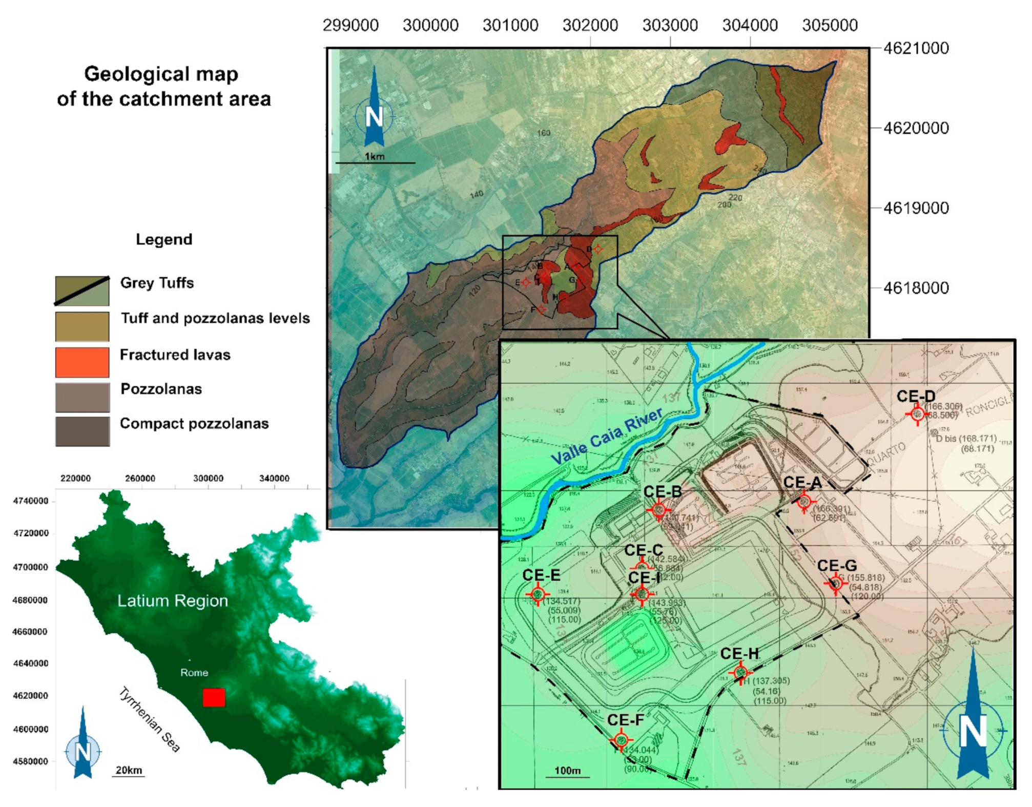
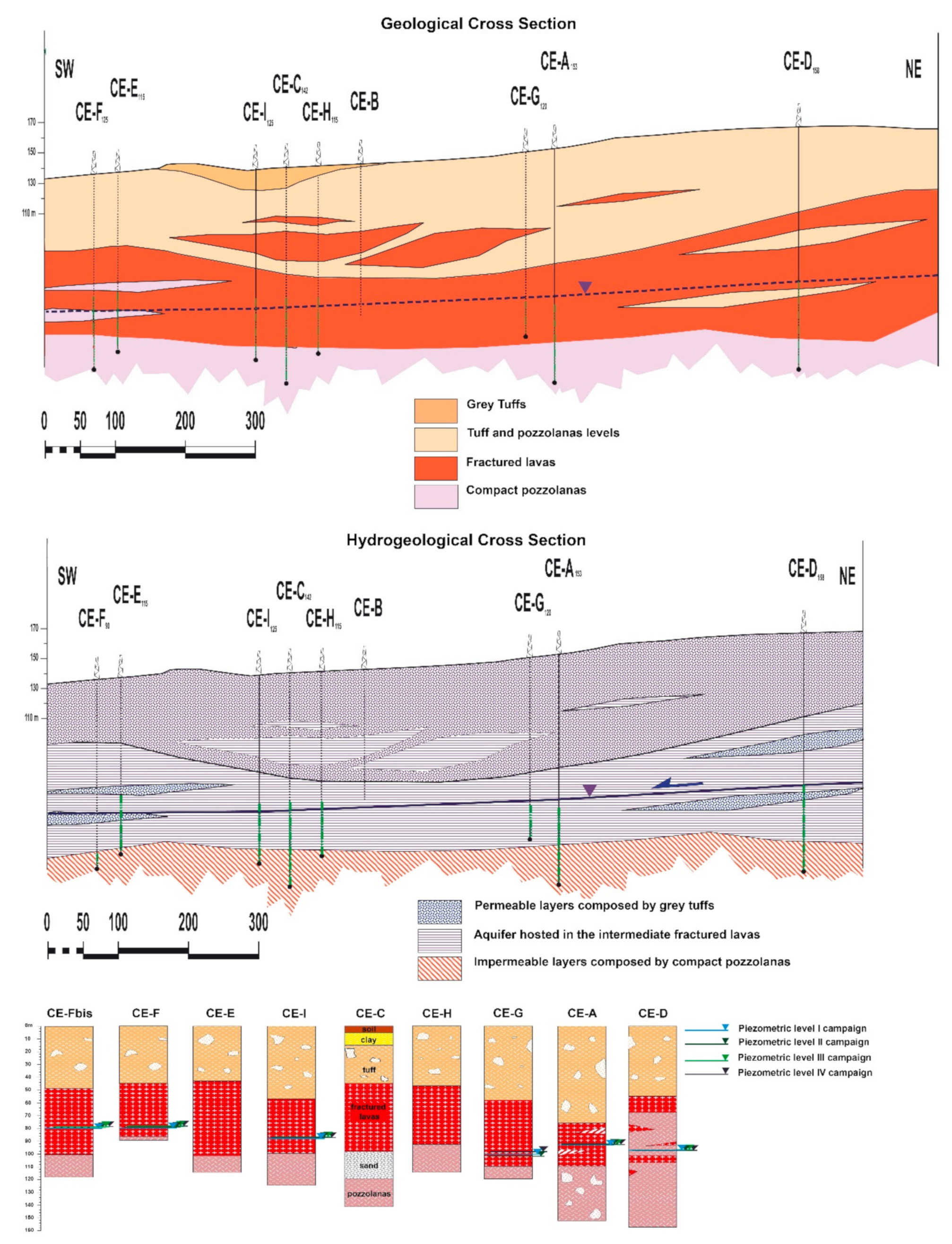
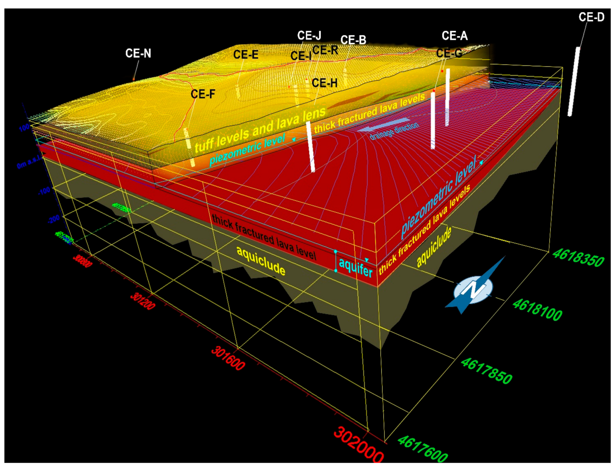
2.1. Geological and Hydrogeological Setting

The investigated area is about 52 ha of which 11 ha comprise waste disposal dumps and the rest treatment facilities (Figure 1). It is located in the South-Western sector of the Colli Albani volcanic district (Albano Laziale, Rome), which is represented by Quaternary volcanisms belonging to the ultrapotassic Roman province [45]. The treatment facility manages waste with a mechanical biological treatment aimed at the production of secondary solid fuel and stabilized organic fraction, and metal recovery. It also manages the biogas collection system and related electricity production facility. The plant is able to treat 500 tons of municipal solid waste per day.

The area is located at the top of the Tuscolano-Artemisio volcanic stage [46,47,48]. Moreover, the outcropping formations are characterized by grey tuffs, fractured lava, and compact pozzolanas. The last, from a hydrological point of view, represents the impermeable layer of the aquifer hosted in the fractured lavas. The groundwater circulation is linked to the extensive Colli Albani main hydrogeological unit [21], characterized by a centrifugal drainage trend around the Albano Lake volcanic complex [49,50]. The whole area is also characterized by several minor perched aquifers maintained by thin waterproof layers represented by compacted tuffs and paleosols. It has long been recognized in literature that the permeability of rocks is extremely variable, from low to high [51,52,53]. This is mainly due to a secondary process, represented by fracturation, which completely changes the hydrogeological behavior of the un-deformed rocks.

2.2. Digital Elevation Model

With the integration of elevation data gathered from topographic maps, aerial photo interpretation and field measurements, a Digital Elevation Model (DEM) was created (Figure 1) using the Surfer10 software.

A rectangular grid (numerical matrix) was realized using the intersection of rows and columns to obtain a three-dimensional representation of the entire drainage basin.

A highly detailed Digital Elevation Model (DEM) was used to automatically map the stream channel and divide the networks of a watershed located in the study area. The construction of a code describing the network topology, each drainage area and the associated stream link represents the basis for an efficient watershed information system. A detailed DEM was superimposed on a thematic slope map and on drainage direction/intensity ones to obtain dynamic surface maps and to identify the local-scale run-off potentially affecting the municipal solid waste disposal site [54,55,56,57].

Meso and macrostructural surveys together with surface and sub-surface geological analyses were carried out to spatially identify the geological structures, geometry, and when possible the fracturation network. The latter represents a fundamental aspect that directly affects the water circulation and facilitates infiltration processes and groundwater circulation.

The DEM was realized with a mesh of 5 meters in order to have a reproduction as close as possible to reality. When necessary, in order to increase the ground resolution of the altimetric variations, the mesh was thickened up to 2 m ground resolution. A geological cross section and block diagram were realized by processing data from the stratigraphical logs of the piezometer used as a monitoring network.

2.3. Groundwater Sampling and on Site Characterization

It was first necessary to depict the dynamicity and complexity of the groundwater flux and identify where contaminant movement to groundwater was concentrated. Therefore, water samples were collected from eight piezometers four times and the main chemical (inorganic and organic contaminants) and quantitative parameters (groundwater regime level) required in both the Italian [58] and European (Water Frame Directive) [32] legislation were measured. An ecological evaluation was performed in addition. It includes the analyses of the groundwater natural microbial community (cell abundance and viability) and the dissolved organic carbon (DOC). Finally, we integrated the overall data with the geological structures in both two and three dimensions.

A preliminary campaign made it possible to select 8 internal piezometers and an external one (Figure 1,

Table 1. Maximum depth, piezometer-top/bottom and diameter, and static water level of the CE-A, CE-B, CE-C, CE-D, CE-E, CE-F, CE-G, CE-H, and CE-I piezometers in the four sampling campaigns (I, II, III and IV). Static level was not measured for CE-E piezometer. a.s.l. = above sea level.

Piezometer	Maximum Depth from Surface (m)	Piezometer-Top/Bottom (m) (a.s.l.)	Diameter (mm)	Static Level (m) (a.s.l.)				Range
				I September	II February	III July	IV October
CE-A	153	156.39/3.39	150	63.5	63.8	63.8	64.2	0.7
CE-B	100	140.74/40.74	150	59.6	59.7	60	60	0.4
CE-C	142	142.58/0.58	250	57.1	57.5	57.8	57.6	0.7
CE-D	158	166.31/8.31	180	68.8	68.9	69.4	69.3	0.6
CE-E	15	134.52/119.52	75	-	-	-	-	-
CE-F	90	134.04/44.04	75	54.2	54.8	56.1	56.1	1.9
CE-G	120	155.82/35.82	75	55.5	53.8	62.8	57.2	7.3
CE-H	115	137.31/20.31	75	54.9	54.2	58.9	56.4	4.7
CE-I	125	143.96/16.96	170	56.2	56.6	56.8	56.6	0.4

). Water samplings for chemical and microbiological analyses and hydrogeological measurements were performed in all piezometers within the municipal solid waste disposal site.

Each single water point was sampled in four campaigns during one year (between 2012 and 2013: I September, II February, III July, IV October) in order to have a multi-temporal analysis of the parameters investigated. Owing to accessibility problems, the CE-G piezometer was sampled only in the third and fourth campaigns. Hydrogeological (piezometric depth-average: 124 m), chemical (main inorganic and organic contaminants), DOC and microbiological data (total microbial abundance and cell viability) were analyzed inside and outside the area studied in order to assess if the water body might be negatively affected by the waste disposal plant.

For this purpose, data from the eight internal piezometers (named CE-A, CE-B, CE-C, CE-E, CE-F, CE-G, CE-H, CE-I) and the external one (CE-D, which is the most upstream one) were compared during 1 year and processed with a geostatistical approach [59,60,61].

For each piezometer the depth-average piezometric level and main physico-chemical parameters (pH, redox potential, electrical conductivity, dissolved oxygen, temperature, and alkalinity) were measured on site using a pre-calibrated multiparameter probe (WTW, Germany) [53,62]. Water samples were collected from each single piezometer after 30 minutes of purging and placed in sterile polyethylene bottles to avoid any contamination. Subsamples were immediately processed for different purposes. For trace elements, dissolved organic carbon (DOC) and main cations and anions, water samples were filtered (0.45 μm) and then put in polyethylene bottles (previously cleaned with HNO₃ and then washed with milliQ water). A pre-acidification of the sample (HNO₃ 1%) was performed before metal and DOC analyses. For organic contaminants, water samples were collected in pre-cleaned 2.5 L dark glass bottles. For microbiological analyses, water samples were immediately fixed with formaldehyde (2% final concentration) for microbial abundance or were kept fresh for microbial cell viability. All the groundwater samples were stored (24 h maximum) at 4 °C before use.

The reconstruction of the piezometric level of the aquifer was performed through the analysis of the static groundwater level using several measuring points consisting of springs, piezometers and equipped piezometers within the municipal solid waste disposal site. These data were processed to obtain a three-dimensional surface, suitable for obtaining a 3D volumetric geometry of the aquifer. All the data were analyzed using geostatistical programs.

2.4. Chemical Analyses

The main inorganic and organic pollutants considered in the WFD [32] and Italian legislation (Decree law 152/06) [58] for evaluating the water quality state were searched for.

Analyses of thirty-two inorganic elements (anions, cations, and metals) were performed in accordance with the Italian Environment Protection Agency Guidelines [63] and APHA, AWWA, WEF methods [64]. Inorganic Anions (Fluoride, Chloride, Nitrite, Nitrate, and Sulfate) were determined by ion chromatography using a Dionex DX-120 Ion Chromatograph. Inductively coupled plasma-mass spectrometry (ICP-MS-Agilent technologies 7500c, Santa Clara, CA, USA) with an Octopole Reaction System (ORS) was used for the determination of Boron, Barium, Antimony, Arsenic, Cadmium, Total Chromium, Copper, Lead, Mercury, Nickel, Selenium, Vanadium, Iron, Zinc, Manganese, Aluminum, Strontium, Lithium, Cesium, Uranium, and Cobalt.

Calcium, Magnesium, Sodium, and Potassium were determined by Inductively Coupled Plasma Optical Emission Spectroscopy (ICP-OES-Perkin Elmer, Waltham, MA, USA) using a Perkin Elmer P400 spectrometer.

Analysis of ninety-two organic contaminants was performed. Polycyclic Aromatic Hydrocarbons (PAH_s) were extracted by SPE (solid-phase extraction) and then determined using a high-performance liquid chromatography (HPLC-Varian 9010-Agilent technologies, Santa Clara, CA, USA) with fluorescence detection (FL-Perkin Elmer LS30-Perkin Elmer, Waltham, MA, USA) [65]. The identity of each analyte was confirmed by liquid chromatography-mass spectrometry (LC-MS) in accordance with Patrolecco et al. [65].

Volatile organic compounds (VOC_s) were determined by the dynamic purge-and-trap technique using a Tekmar dynamic purge-and-trap system (Teledyne Tekmar, Mason, OH USA), equipped with a 25 mL glass vessel, coupled to a gas Saturn 2200 (Varian) chromatograph/mass spectrometric system (GC/MS-Agilent technologies, Santa Clara, CA, USA). An aliquot of 25 mL of the water sample was manually introduced into the vessel using a syringe. The VOCs purged by a helium flow were trapped onto a Tenax cartridge and then thermally desorbed at 210 °C and swept to the GC column were they were separated and detected by the MS system. LODs obtained were between 0.005 and 0.1 µg/L depending on the VOC selected.

Chlorinated pesticides were extracted applying solid-phase extraction (SPE) and then determined by gas chromatography (GC) with an electron capture detector (ECD) using Perkin Elmer, Clarus 480 and a fused silica capillary column [66].

The list of overall organic compounds analyzed in the groundwater samples is reported in

Table 2. List of organic contaminants examined in the nine piezometers sampled.

Group of Organic Contaminants	Chemicals
Polycyclic Aromatic Hydrocarbons (PAHs)	Naphthalene, Acenaphthene, Fluorene, Phenanthrene, Anthracene, Fluoranthene, Pyrene, Benzo(a)Anthracene, Chrysene, Benzo(b)fluoranthene, Benzo(k)fluoranthene, Benzo(a)pyrene, Dibenz(a,h)anthracene, Benzo(g,h,i)perylene, Indeno(1,2,3-c,d)pyrene, Dibenzo(a,e) pyrene, Dibenzo(a,i) pyrene, Dibenzo(a,h) pyrene, Dibenzo(a,l) pyrene
Volatile Organic Compounds (VOCs)	Trichloromethane, Tribromomethane, 1,2-Dibromoethane, Dibromochloromethane, Bromodichloromethane, 1,2-Dichloroethane, 1,1-Dichloroethane, 1,2-Dichloropropane, 1,1,2-Trichloroethane, 1,2,3-Trichloropropane, 1,1,2,2-Tetrachloroethane, Chloroethene, Chloromethane, 1,2-Dichloroethene, 1,1-Dichloroethene, Trichloroethylene, Tetrachloroethylene, Hexachloro-1,3-butadiene, Chlorobenzene, 1,2-Dichlorobenzene, 1,3-Dichlorobenzene, 1,4-Dichlorobenzene, 1,2,4-Trichlorobenzene, 1,2,3-Trichlorobenzene, n-Hexane, Benzene, Ethylbenzene, Styrene, Toluene, ortho-Xylene, meta-Xylene, para-Xylene, (1-methylethyl)benzene, Propylbenzene, Methylbenzene, Bromobenzene, Phenylamine, Diphenylamine, o-Toluidine, prop-2-enamide, pyridine-3-carboxylic acid, 1,2-Dinitrobenzene, 1,3-Dinitrobenzene, 1-methyl-2,4-dinitro benzene, n-Nitrotoluene, 1-Chloro-2-nitrobenzene, 1-Chloro-3-nitrobenzene,1-Chloro-4-nitrobenzene, 1,2,3-Trichloropropane, Dichloromethane, Bromomethane, Tetrachloromethane, Chloroethane, Dichlorodifluoromethane, Trichlorofluoromethane, Bromoethene, 1-bromo-2-chloroethane, Dichlorobutane, 1,1,1-Trichloroethane, 1,1,1,2-Tetrachloroethane, Bromodichloroethane, 4-Bromochlorobenzene, 1,1-Dichlorocycloutane, 1,4-Dichlorobut-2-ene, 2-Methoxy-2-methylpropane, Diiodomethane, n- Propylbenzene
Chlorinated Pesticides	Dichlorodiphenyldichloroethylene (DDE) Gamma-hexachlorocyclohexane (γ HCH)

.

2.5. Dissolved Organic Carbon (DOC)

Aliquots of water samples (20–500 µL) were analyzed for dissolved organic carbon content with high temperature catalytic oxidation using a Shimadzu TOC-5000A Total Organic Carbon Analyzer, with a detection limit of 0.15 mg/L.

2.6. Microbiological Analysis

The microbial abundance (No. cells/mL) was determined in at least four replicates in each piezometer. Water aliquots (20 mL) fixed in formaldehyde (2%) were filtered on black polycarbonate filters (pore size 0.22 µm, 25 mm diameter) and stained for 20 minutes at 4 °C in the dark with the DNA intercalant DAPI (at the final concentration of 1 µg/L). Finally, the filters were observed under an epifluorescence microscope (Leica DM 4000B). The DAPI method was used because it is able to detect all the microbial cells in a sample whatever their physiological state and metabolic activity and for this reason is suitable for the total microbial counts [67,68].

Cell viability (% live cells/live + dead) was measured in four fresh replicate subsamples (20 mL each) using two fluorescent dyes. SYBR Green II and propidium iodide (Sigma-Aldrich, Germany) were used for distinguishing between viable (green) and dead or damaged (red) cells under a fluorescence microscope [34]. The cells were counted in both analyses with the epifluorescence microscope at 1000 magnification, counting a minimum of 300 cells per filter. Each microbiological measure was the average of four replicate filters comprising at least 1200 microbial cells counted.

2.7. Statistical Analysis

The statistical analysis was performed, using the R software version 2.15 (downloaded from the Comprehensive R Archive Network (CRAN), which is located at http://cran.r-project.org/). The t test was used to compare the overall organic contaminant concentrations among the different piezometers. Moreover, any correlations between DOC and abiotic (conductivity, dissolved oxygen, bicarbonates, ∑ organic contaminants, PAHs, VOCs) and biotic (microbial abundance and cell viability) parameters, whatever the piezometer location and the sampling time, were also evaluated.

2.8. Geostatistical Analysis

In order to investigate the distribution and evolution patterns of pollutants in the groundwater an ordinary kriging [69,70,71] was performed taking into consideration the overall data obtained from the sampling, using the Surfer10 software.

This method consists of a spatial interpolation technique, which makes it possible to obtain contour distribution maps. Among the numerous geostatistical gridding methods that are useful in many fields of applications, kriging provides visually appealing maps from irregularly spaced data and incorporates anisotropy and underlying trends in an efficient and natural manner [72]. Moreover, kriging is very flexible and makes it possible to obtain spatial autocorrelation graphs, allowing prediction, prediction standard errors, and probability maps, minimizing at the same time errors in predicted values. To measure the mean variability between two sampled points x and x + h, as a function of their distance h semi-variograms were produced. The semi-variogram is an autocorrelation statistic defined as follows:

$$\hat{y}(h) = \frac{1}{2n}{{\displaystyle \sum }}_{i=1}^n{(z\left(x_i\right)-z(x_i+h))}^2$$

where n is the number of pairs of sample points separated by distance h, z(x_i) is the value of the variable z at point i, and z(x_i + h) is the value of the variable z at point i + h. The assumptions of kriging are a stationary difference between x and x + h and variance of the differences, which define the requirements for the intrinsic hypothesis. This means that semi-variance does not depend on the location of samples and only depends on the distance between samples, so that the semi-variance is isotropic. Consequently, several geostatistic thematic maps of the site were made using the most suitable model with the least errors.

3. Results

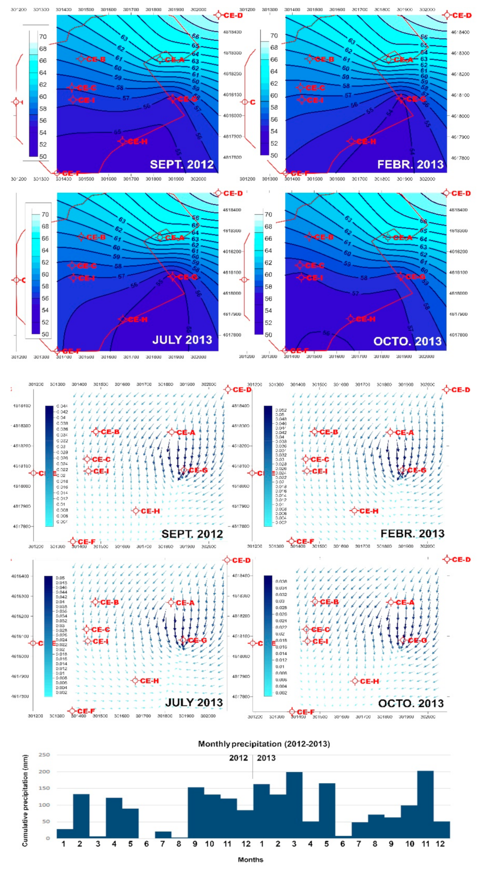
3.1. Geological and Hydrogeological Characterization

The reconstruction of a detailed geological cross section (Figure 2) allows us to identify the limit of the aquiclude represented by the “Pozzolane inferiori” formation. Using the surface geological and geometrical data acquired directly in the field and well log stratigraphy it was possible to correlate and model the complete volcanic sequences observed in the area investigated. Furthermore, each single geologic unit was geometrically identified and superimposed on the others to obtain a complete 3D picture of the whole volcanic template succession using the Voxler3 software. In fact, the overall volcanic sequence lies in an unconformity above a thick sedimentary succession mainly represented by clay, sand, and silt. Heterogeneity of the geological substrata is represented by the alternation between tuff levels and lava lenses in the upper half portion of the cross section (between 0 and 50 m), while the lower half one is characterized by thick fractured lava levels. The latter are characterized by constant thickness in the NE–SW direction and by important lateral thickness variations in the W–E direction. This aspect represents an important factor that strongly limits water circulation towards West and East.

With a total thickness of 30–35 m and a widespread areal distribution, the aquifer located in the thick fractured lavas and supported by compact pozzolanas, which act as an aquiclude (Figure 2 and Figure 3), represents a fundamental element able to rapidly convey pollutants toward SSW, driven by the main drainage direction (Figure 4). The 3D geological and hydrogeological model [73,74,75,76] allows us to better define the vertical and lateral variations of each single rock body [73,74,75,76,77,78]. Because both the fractured lavas and the tuff layers do not show a constant thickness in the whole area studied, it is fundamental to build up a detailed geometry of the volcanic deposits, showing a progressive reduction of the thickness towards both West and South. The latter aspect is key to a better understanding of the hydraulic behavior of the aquifer and a better identification of the relationships between the dump activities, water circulation and bacterial behavior.

The reconstruction of the piezometric level shows a time-space variation with a progressive increase in the water level from 68.5 m (I campaign) to 69.3 m (IV campaign) at piezometer CE-D, which is the upstream of the overall piezometers sampled (Table 1).

The piezometric variation shows a trend that does not seem influenced by seasonal variation, as highlighted by the high level of the piezometric level measured during the February 2013 campaign in the upper stream sector. Despite the vertical variation observed, the drainage direction remained constant during the investigation period showing a main drainage direction from N-NE to S-SW. During the last campaign, the southern sector was characterized by a counterclockwise rotation of the drainage direction toward South. This process was mainly observable within the area comprising the CE-F, CE-H, and CE-I piezometers, as shown in Figure 4.

It is important to underline that the groundwater drainage direction did not have a uniform trend; the gradient in the northern sector (CE-D, CE-A, CE-B, CE-C, CE-I piezometers) was higher than that in the southern sector (CE-F, CE-H, CE-G piezometers) (Figure 4). This result can be ascribed to the inhomogeneities in the permeability profile affecting the groundwater level. Based on the subsurface geological analysis, the CE-B piezometer was the most vulnerable to the waste disposal occurrence owing to the presence of several fractured lava layers between the surface and groundwater levels. This makes possible a passive transport of both organic matter and contaminants from surface to groundwater. On the contrary, the CE-D piezometer was intrinsically less vulnerable because it was located upstream and outside the waste disposal area and was characterized by a vertical geological homogeneity with a low fracturation process. For this reason, it was considered a control piezometer.

3.2. Main Chemical–Physical Parameters on Site

Temperature and pH in all piezometers were quite constant (Supplementary Materials Table S1), with no significant differences between different sampling times and piezometers, with average values of 17.54 ± 0.09 °C and 7 ± 0.03, respectively. Conductivity and dissolved oxygen values are reported in

Table 3. Conductivity (µS/cm) and dissolved oxygen (mg/L) found in each piezometer (CE-A, CE-B, CE-C, CE-D, CE-E, CE-F, CE-G, CE-H, and CE-I) at each sampling campaign.

Piezometer	Conductivity (µS/cm)				Dissolved Oxygen (mg/L)
	I September	II February	III July	IV October	I September	II February	III July	IV October
CE-A	704	1404	789	758	9.14	8.30	8.8	4.3
CE-B	1029	1022	1028	1039	3.3	3.50	3.2	3.3
CE-C	855	905	847	840	8.1	5.2	4.0	7.5
CE-D	718	1412	713	710	8.87	8.9	8.9	8.8
CE-E	713	707	709	718	6.8	6.58	5.1	6.4
CE-F	1039	1040	1035	1049	4.4	3.64	3.7	3.7
CE-G	-	850	862	-	-	6.97	5.1	-
CE-H	850	843	790	798	3.54	6.28	7.5	7.4
CE-I	769	792	770	774	6.5	6.73	6.7	7.3

and Table S1 (Supplementary Materials).

The highest values for conductivity and the lowest for oxygen were in the CE-B and CE-F piezometers. All the other parameters are reported in Supplementary Materials Table S1.

3.3. Chemical Analysis

Anion and cation concentrations found in the four samplings rarely exceeded the corresponding threshold limits required by the Italian legislation (D.Lgs 152/2006 Annex 5; D.Lgs 30/2009, Annex 3), as can be seen in

Table 4. Minimum (Min) and maximum (Max) concentrations of anions and cations found in the four sampling campaigns (second and third column); threshold limits reported in the Italian legislations (fourth column); Numbers of exceeding values and corresponding piezometers (fifth and sixth column).

Ions	Min	Max	Legal limits *	>Limits	Piezometers
Fluorides	0.86	6.64	1.5 mg/L	11	CE-C; CE-E; CE-H; CE-I
Nitrites	0	0	0.5 mg/L	0
Sulphates	19.1	40.39	250 mg/L	0
Be	0.1	0.9	4 μg/L	0
B	114	803.54	1000 μg/L	0
Al	3.1	1718	200 μg/L	8	CE-E; CE-F; CE-G; CE-H
Cr Tot	0.8	3.7	50 μg/L	0
Cr (VI)	<0.5	<0.5	5 μg/L	0
Mn	0.2	46.2	50 μg/L	0
Fe	7.5	543	200 μg/L	3	CE-G; CE-H
As	8.3	26.58	10 μg/L	28	CE-A; CE-B; CE-C; CE-E; CE-F; CE-G; CE-H; CE-I
Ni	0.3	7.8	20 μg/L	0
Cu	0.21	4.53	1000 μg/L	0
Co	0.3	2.5	50 μg/L	0
Zn	2.5	838	3000 μg/L	0
Se	0.1	0.6	10 μg/L	0
Ag	<0.1	<0.1	10 μg/L	0
V	30.2	49.8	50 μg/L	0
Cd	0.11	0.15	5 μg/L	0
Sb	0.2	0.4	5 μg/L	0
Hg		<0.1	1 μg/L	0
Pb	0.1	1.5	10 μg/L	0

* D.Lgs 152/06; D.Lgs 30/2009, Annex 3.

and in detail in Supplementary Materials (Table S1).

Nitrites were never found and the legislation limits for inorganic elements were exceeded only in the case of fluorides (>1.5 mg/L), aluminum, iron and arsenic in several piezometers (Supplementary Materials Table S1). However, these values were in line with those naturally found in volcanic areas of Central Italy and can therefore be ascribed to a geogenic origin [53,79].

The overall chemical analysis results (see Supplementary Materials, Tables S2, S3, and S4) showed that although 92 contaminants were searched for, only 31 were found in residual concentrations. The legislation limit (0.15 µg/L) for the volatile organic compound 1,2 Dichloropropane was exceeded just in the case of CE-B (0.17 µg/l) and CE-F (0.55 µg/L) piezometers in the third campaign (July), (Table S4).

However, in order to assess a possible impact from the waste dump and the groundwater vulnerability to residual multiple contamination, at each single piezometer sampled, the residual concentrations of each single compound were added together and a “sum value” is reported for each single piezometer in

Table 5. Sum value of all organic contaminants (μg/L) found in each piezometer (CE-A, CE-B, CE-C, CE-D, CE-E, CE-F, CE-G, CE-H, and CE-I) and at each sampling.

Piezometer	I September (µg/L)	II February (µg/L)	III July (µg/L)	IV October (µg/L)
CE-A	0.398	0.122	0.434	0.287
CE-B	0.813	0.238	1.08	0.597
CE-C	0.508	0.129	0.92	0.353
CE-D	0.312	0.049	0.674	0.259
CE-E	0.291	0.061	0.465	0.236
CE-F	0.667	0.529	1.579	-
CE-G	0.646	0.163	0.347	0.179
CE-H	0.651	0.121	-	0.546
CE-I	0.398	0.219	1.12	0.288

.

In the first sampling, 15 micro-contaminants were found (trichloroethylene and tetrachloroethylene were in all piezometers sampled); however, the legislation limits were never exceeded. The highest number of contaminants and the highest sum value were found at the CE-B piezometer (0.8 μg/L: VOCs 0.78 μg/L + PAHs 0.021 μg/L), followed by the CE-F (0.7 μg/L: VOCs 0.66 μg/L + PAHs 0.04 μg/L), CE-H (0.65 μg/L: VOCs 0.633 μg/L + PAHs 0.016 μg/L) and CE-I (0.4 μg/L: VOCs 0.38 μg/L + PAHs 0.022 μg/L).

In the second sampling, 21 micro-contaminants were found, although their concentrations were very low. The highest sum values were found at the CE-F piezometer (0.53 μg/L: 0.13 μg/L VOCs + 0.4 μg/L PAHs) and at the CE-B one (0.24 μg/L: 0.09 μg/L VOCs + 0.15 μg/L PAHs), respectively.

In the third sampling (July) 22 micro-contaminants were found and their sum values were significantly higher (t test, p < 0.01) than those in the two previous samplings. In particular, at the CE-F piezometer the sum value of all contaminants was 1.58 µg/L (1.56 µg/L for VOCs and 0.016 µg/L for PAHs) and at the CE-B piezometer 1.08 µg/L (only VOCs were found). In this sampling, beyond the most frequently found Trichloroethylene, Tetrachloroethylene, 1,2-Dichloropropane, Etilbenzene, o/p-Xilene, and Phenantrene were also found (Tables S3 and S3). However, the legislation limit (0.15 µg/L) was exceeded just for the volatile organic compound 1,2-Dichloropropane at both the CE-B (0.17 μg/L) and CE-F (0.55 μg/L) piezometers.

In the fourth sampling (October) 15 micro-contaminants were found; 1,2-Dichloropropane was found at the CE-B, CE-C, CE-F, and CE-I piezometers, however its concentrations were always in trace amounts (Tables S2 and S3), below the legislation limit.

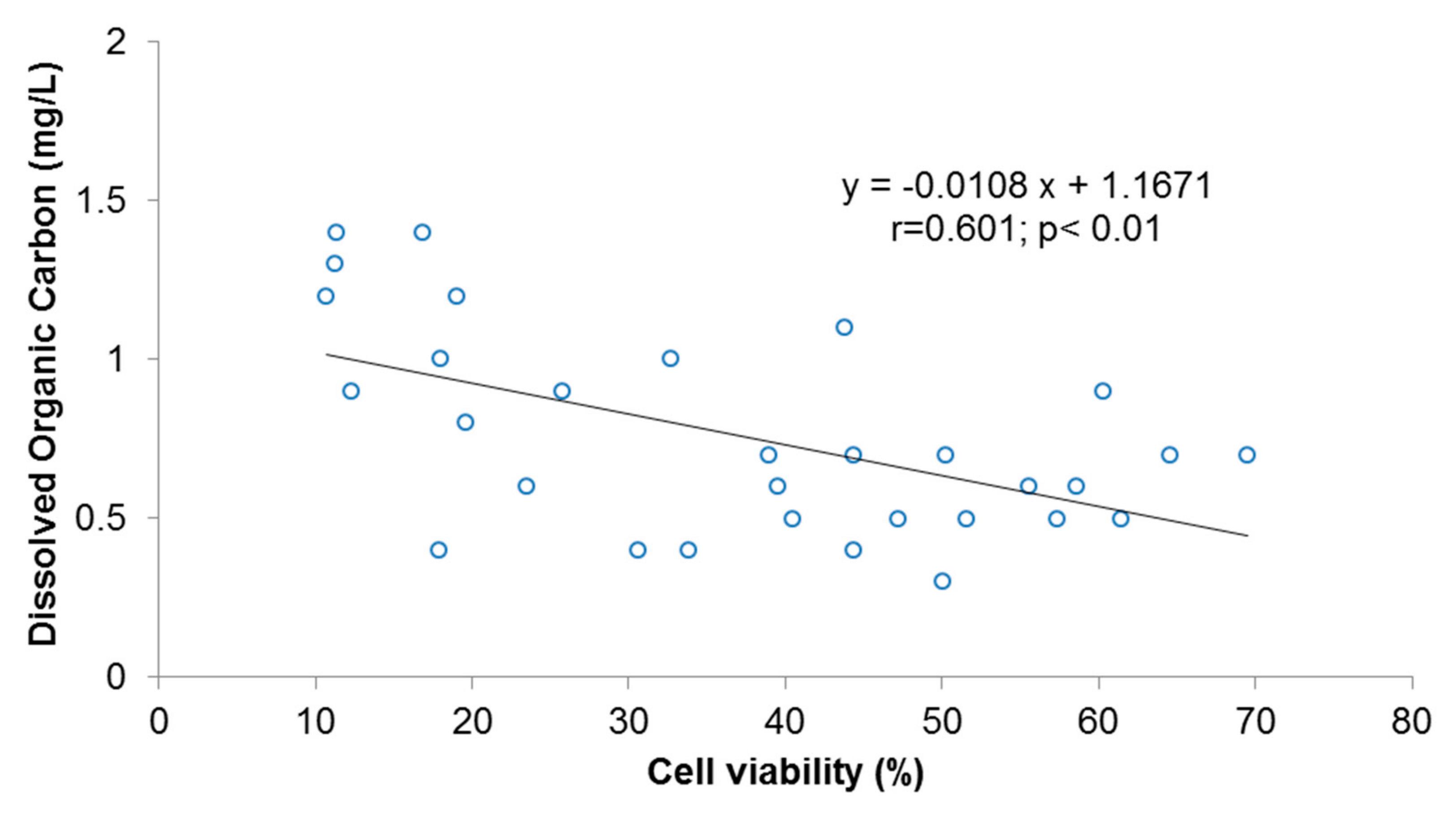
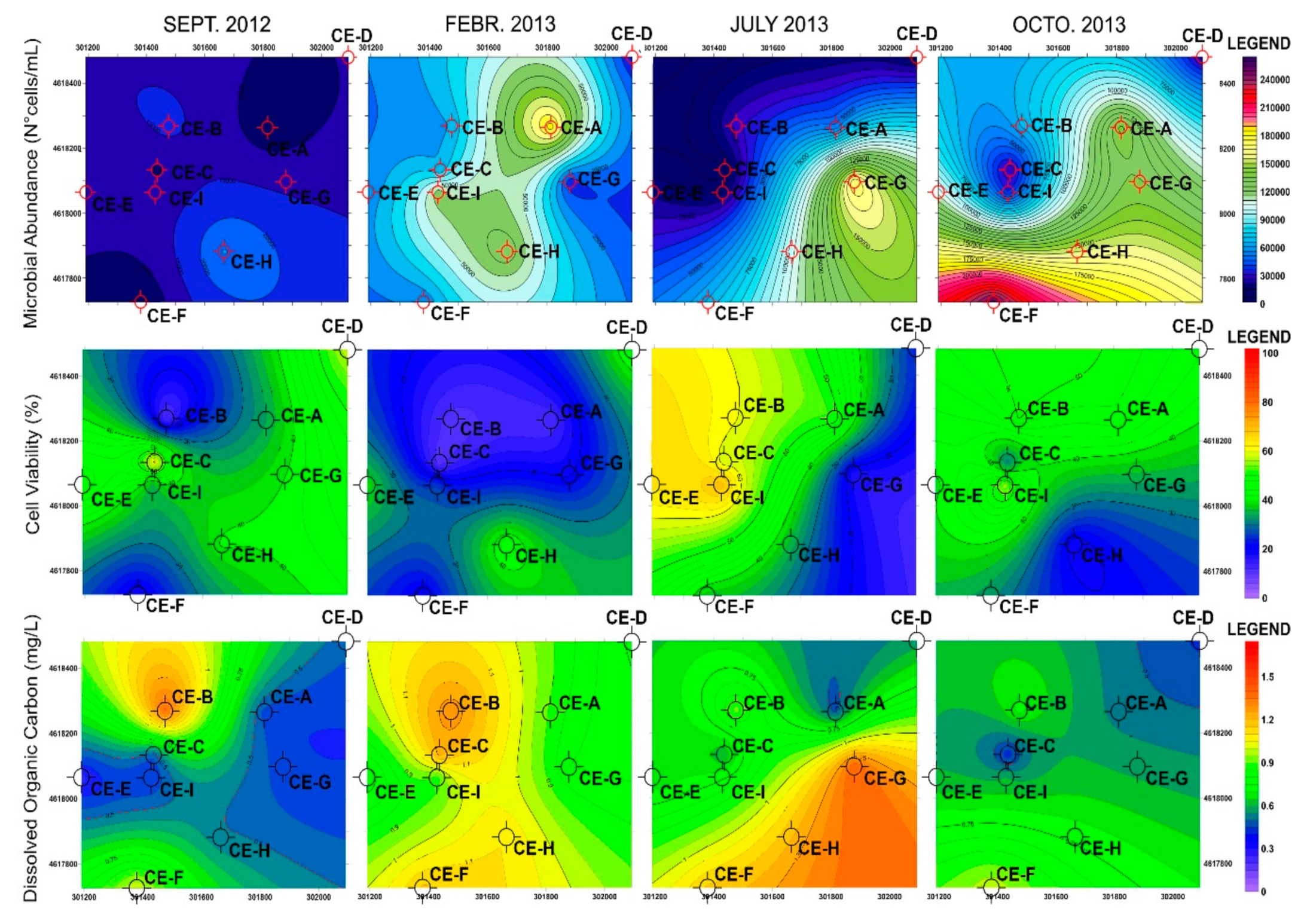
3.4. Dissolved Organic Carbon

The average value of DOC was 0.6 mg/L ± 0.1 at the CE-D piezometer located upstream from the dump and at the CE-A and CE-E piezometers located on the boundary of the dump; the DOC values were significantly higher (p < 0.05) (ranging from 0.7 to 1.1 mg/L) at the other piezometers (CE-B, CE-C, and CE-F). No relationships were found between the DOC values and sum values of all organic contaminants; while a positive relationship was found between DOC and dissolved oxygen and conductivity (p < 0.01) (

Table 6. Dissolved Organic Carbon (DOC) values determined in each piezometer (CE-A, CE-B, CE-C, CE-D, CE-E, CE-F, CE-G, CE-H, and CE-I) at each sampling campaign.

Piezometer	DOC (mg/L)
	I September	II February	III July	IV October	Average	±se
CE-A	0.4	0.9	0.5	0.5	0.6	±0.1
CE-B	1.4	1.3	0.9	0.7	1.1	±0.2
CE-C	0.5	1.2	0.6	0.4	0.7	±0.2
CE-D	0.5	0.7	0.6	0.4	0.6	±0.1
CE-E	0.3	0.7	0.7	0.6	0.6	±0.1
CE-F	1.0	1.2	1.2	1.0	1.1	±0.0
CE-G	0.4	0.8	1.4	0.6	0.8	±0.3
CE-H	0.5	1.1	2.0	0.7	1.1	±0.3
CE-I	0.4	0.9	0.7	0.6	0.7	±0.1

).

3.5. Microbial Abundance and Cell Viability

The microbial abundance values (No. cells/mL) ranged from a minimum of 5.3 × 10³ ± 1.3 × 10³ to a maximum of 1.2 × 10⁶ ± 7.7 × 10⁴ (

Table 7. Microbial abundance (No. Cells/mL) values determined in each piezometer (CE-A, CE-B, CE-C, CE-D, CE-E, CE-F, CE-G, CE-H, and CE-I) at each sampling campaign.

Piezometer	Microbial Abundance (No. Cells/mL)
	I September	II February	III July	IV October	Average	±se
CE-A	6.9 × 103	8.8 × 104	5.2 × 104	1.4 × 105	7.2 × 104	±2.9 × 104
CE-B	1.7 × 104	3.1 × 104	2.9 × 104	6.6 × 104	3.6 × 104	±1.1 × 104
CE-C	9.2 × 103	3.1 × 104	9.0 × 103	2.6 × 104	1.9 × 104	±5.7 × 103
CE-D	1.0 × 104	1.4 × 104	1.2 × 104	2.2 × 104	1.4 × 104	±2.5 × 103
CE-E	1.5 × 104	2.6 × 104	1.9 × 104	1.1 × 105	4.2 × 104	±2.2 × 104
CE-F	5.3 × 103	2.6 × 104	6.6 × 104	2.5 × 105	8.8 × 104	±5.7 × 104
CE-G	-	1.7 × 104	1.7 × 105	-	9.4 × 104	±7.7 × 104
CE-H	2.5 × 104	6.5 × 104	1.5 × 104	1.2 × 106	3.3 × 105	±2.9 × 105
CE-I	1.2 × 104	5.8 × 104	1.5 × 104	3.5 × 104	3.0 × 104	±1.1 × 104

). The CE-D piezometer had the lowest average value if compared with the other ones.

The cell viability values (expressed as % live cells/live + dead) ranged from 10.7% to 69.5% (

Table 8. Cell viability (% live cells/live + dead) values determined in each piezometer at each sampling campaign.

Piezometer	Cell Viability (%)
	I September	II February	III July	IV October	Average	±se
CE-A	33.8	12.3	51.5	47.2	36.2	±8.8
CE-B	11.3	11.2	60.3	50.2	33.2	±12.9
CE-C	61.4	10.7	58.6	30.6	40.3	±12.1
CE-D	57.3	44.3	23.5	44.3	42.3	±7.0
CE-E	50.0	38.9	64.5	39.5	48.2	±6.0
CE-F	18.0	19.0	37.1	32.7	26.7	±4.8
CE-G	-	19.6	16.8	-	18.2	±1.4
CE-H	40.4	43.8	-	18	34.1	±8.1
CE-I	34.9	25.7	69.5	55.5	46.4	±12.2

). The data for the CE-H piezometer regarding the third sampling are not reported, owing to the interference of suspended particles, which hampered cell observations under the microscope.

A significant negative correlation was found (p < 0.01) between the cell viability and DOC values (Figure 5).

3.6. Spatial and Multi-Parameter Monitoring over 1 Year with 4 Season Analysis

Data collected were used for the geostatistical analysis. Close relationships among the geological heterogeneity, water circulation, pollutant diffusion, dissolved organic carbon, and cell viability were found. The thematic maps regarding microbial abundance, cell viability, and DOC are reported with a chromatic scale in Figure 6.

Microbial abundance was not directly related either to cell viability or to the DOC values (Figure S1). On the contrary, a close relationship (p < 0.01) was found between cell viability and dissolved organic carbon. The highest values for cell viability were found with DOC values ≤ 0.5 mg/L; above these values DOC seems to negatively affect the microbial community (Figure 5).

4. Discussion

The study carried out allowed us to reconstruct in detail the surface and subsurface geological structure of the investigated area. Using field analyses, piezometer stratigraphy (when available) and computer modelling, a new and up to date 3D geological model of the area was performed. The latter, mainly composed of a layer cake template succession of tuffs, lavas and compacted pozzolanas, with a total thickness up to 300 m, was characterized by a shallow aquifer comprised within the lava layers. A detailed structural analysis carried out on the outcropping formation showed an intense fracturation process, which substantially modified, as a second order process, the first order mechanical and hydraulic characters of the rocks (very low permeability). This last aspect is key to a better understanding of water circulation and drainage directions. The brittle deformation processes involving the most rigid formations of the entire stratigraphic succession are characterized by piezometer-organized and sub-parallel extensional fracture lineaments, showing different overlapped generations. In particular, the intersection among different fracture systems represents a preferential water vertical direction flux from the surface through the volcanic succession to the aquiclude levels, composed of the compact pozzolanas layers. However, the fracturation processes, which are not evenly distributed either planimetrically or vertically, favor the development of areas with higher induced permeability (secondary permeability) values such as those at CE-B and CE-F piezometers. Using the computer modelling software, it was possible to model the geological structures in the area investigated in 3D and evaluate the direction, geometry and volumes of both groundwater and volcanic formations. In this configuration, the surface successions of tuffs, unevenly fractured, represent the unsaturated layers, which should perform the function of protecting aquifers from contamination processes coming from the surface. Despite this, the pervasive fracturation processes, which also affects the tuffs, can make it possible for chemicals to directly reach the aquifer.

The overall data analysis regarding the 6 piezometers belonging to this volcanic aquifer showed that the threshold values for evaluating the chemical and quantitative status established by the European WFD and entered in force in the Italian legislation [32,58] were not exceeded, except for one chemical at two points (CE-B and CE-F) in the July sampling campaign. Using the current legislation approach, we can state that the waste dump did not negatively affect the groundwater quality.

However, by considering unconventional parameters such as DOC and cell viability and applying a geostatistical analysis we were able to identify some points where the groundwater was unexpectedly vulnerable to inputs from the surface. In this context, the high DOC value observed for the most vulnerable piezometer CE-B, whatever the season, can be ascribed to the dump’s presence. Using our approach, we identified the initial carbon input peak, at the CE-B piezometer, (September and February) and its transfer with the subsurface water flow in the following months toward the Southern sector of the area investigated though groundwater circulation. In fact, a progressive increase in DOC values during time at the CE-G (February and July), CE-H (February–July) and, downstream, CE-F piezometers (July and October) was observed (Figure 6).

An opposite trend was found for the cell viability (highest DOC, lowest viability), showing that DOC values above 0.6 mg/L had a detrimental effect on the groundwater microbial community (Figure 6). In fact, in the external control piezometer CE-D, DOC always displayed relatively low values, in accordance with those commonly found in pristine groundwater [1,34]. A low DOC content is known to be a factor limiting the growth of bacterial communities; on the contrary, in our samples we observed that the lowest cell viability was associated with the highest DOC values. This suggests that the additional organic carbon comes from the dump and that the microbial communities are sensitive to its origin and quality. This result, showing the negative effects on the microbial community of higher values of DOC in contaminated ecosystems, is in line with those found in in previous works [80,81,82]. Finally, it is interesting to note that in the third sampling campaign the lowest oxygen concentrations were found and the volatile organic compound 1,2 Dichloropropane detected above the legislation limits in the most vulnerable piezometers (CE-B and CE-F). The presence of volatile organic compounds is an indicator of anthropogenic activities [83]. Negative effects on the microbial community due to high DOC values and trace contamination of chlorinated organics were found in previous studies in groundwater [80]. These results show that a contaminant threshold compliance alone does not exclude possible effects from the trace contaminant mixture on the groundwater ecosystem. Once the most vulnerable groundwater sectors are identified, monitoring surveys can focus on these points and also take into consideration the microbiological parameters.

5. Conclusions

The overall results show that the chemical analysis of single contaminants and quantitative parameters required by the current regulations is not always able to assess the vulnerability of a groundwater and all the possible impacts of a waste deposit area. On the contrary, a detailed geological and hydrogeological analysis made it possible to understand the surface and subsurface geological structures of the area investigated. The new 3D geological model made it possible to identify the geometry and distribution of the different volcanic formations in the area studied. The meso-structural analysis showed different extensional fracture generations affecting both the tuffs and lavas. The intersection among different fracture lineament generations represents a preferential pathway for chemicals and organic carbon to reach and affect groundwater. This process was evident in the most vulnerable CE-B and CE-F piezometers. This study also shows that the geostatistical analysis makes it possible to understand the relationships between parameters and spatial heterogeneity in a better way than the classic statistical analysis. Finally, unconventional ecological parameters such as cell viability and DOC can be more sensitive than the chemical determinations alone for assessing the anthropogenic pressure on an aquifer and can be good indicators of water quality to be added to those required by the current legislation.

References

1. Barra Caracciolo, A.; Fajardo, C.; Grenni, P.; Sacca’, M.L.; Amalfitano, S.; Ciccoli, R.; Martin, M.; Gibello, A. The role of a groundwater bacterial community in the degradation of the herbicide terbuthylazine. FEMS Microbiol. Ecol. 2010, 71, 127–136. [Google Scholar] [CrossRef] [PubMed]
2. European Commission Water Statistics-Share of External Inflow from Neighbouring Territories in Renewable Freshwater Resources-Long-Term Annual Average. Available online: https://ec.europa.eu/eurostat/statistics-explained/index.php/Water_statistics (accessed on 9 May 2019).
3. Ducci, D.; de Melo, M.T.C.; Preziosi, E.; Sellerino, M.; Parrone, D.; Ribeiro, L. Combining natural background levels (NBLs) assessment with indicator kriging analysis to improve groundwater quality data interpretation and management. Sci. Total Environ. 2016, 569–570, 569–584. [Google Scholar] [CrossRef] [PubMed]
4. Preziosi, E.; Parrone, D.; Del Bon, A.; Ghergo, S. Natural background level assessment in groundwaters: Probability plot versus pre-selection method. J. Geochem. Explor. 2014, 143, 43–53. [Google Scholar] [CrossRef]
5. Looser, M.; Parriaux, A.; Bensimon, M. Landfill underground pollution detection and characterization using inorganic traces. Water Res. 1999, 33, 3609–3616. [Google Scholar] [CrossRef]
6. Lapworth, D.J.; Baran, N.; Stuart, M.E.; Ward, R.S. Emerging organic contaminants in groundwater: A review of sources, fate and occurrence. Environ. Pollut. 2012, 163, 287–303. [Google Scholar] [CrossRef] [PubMed] [Green Version]
7. Castañeda, S.S.; Sucgang, R.J.; Almoneda, R.V.; Mendoza, N.D.S.; David, C.P.C. Environmental isotopes and major ions for tracing leachate contamination from a municipal landfill in Metro Manila, Philippines. J. Environ. Radioact. 2012, 110, 30–37. [Google Scholar] [CrossRef] [PubMed]
8. Samadder, S.R.; Prabhakar, R.; Khan, D.; Kishan, D.; Chauhan, M.S. Analysis of the contaminants released from municipal solid waste landfill site: A case study. Sci. Total Environ. 2017, 580, 593–601. [Google Scholar] [CrossRef] [PubMed]
9. Preziosi, E.; Frollini, E.; Zoppini, A.; Ghergo, S.; Melita, M.; Parrone, D.; Rossi, D.; Amalfitano, S. Disentangling natural and anthropogenic impacts on groundwater by hydrogeochemical, isotopic and microbiological data: Hints from a municipal solid waste landfill. Waste Manag. 2019, 84, 245–255. [Google Scholar] [CrossRef] [PubMed]
10. Gogu, R.C.; Dassargues, A. Current trends and future challenges in groundwater vulnerability assessment using overlay and index methods. Environ. Geol. 2000, 39, 549–559. [Google Scholar] [CrossRef]
11. Civita, M.; De Maio, M. Assessing and mapping groundwater vulnerability to contamination: The Italian “combined” approach. Geofis. Int. 2004, 43, 513–532. [Google Scholar] [CrossRef]
12. Tuxen, N.; Albrechtsen, H.-J.; Bjerg, P.L. Identification of a reactive degradation zone at a landfill leachate plume fringe using high resolution sampling and incubation techniques. J. Contam. Hydrol. 2006, 85, 179–194. [Google Scholar] [CrossRef] [PubMed]
13. de Lipthay, J.R.; Tuxen, N.; Johnsen, K.; Hansen, L.H.; Albrechtsen, H.-J.; Bjerg, P.L.; Aamand, J. In Situ Exposure to Low Herbicide Concentrations Affects Microbial Population Composition and Catabolic Gene Frequency in an Aerobic Shallow Aquifer. Appl. Environ. Microbiol. 2002, 69, 461–467. [Google Scholar] [CrossRef] [PubMed]
14. Naidu, R. Recent Advances in Contaminated Site Remediation. Water Air Soil Pollut. 2013, 224, 1573–2932. [Google Scholar] [CrossRef]
15. Safonov, A.V.; Babich, T.L.; Sokolova, D.S.; Grouzdev, D.S.; Tourova, T.P.; Poltaraus, A.B.; Zakharova, E.V.; Merkel, A.Y.; Novikov, A.P.; Nazina, T.N. Microbial Community and in situ Bioremediation of Groundwater by Nitrate Removal in the Zone of a Radioactive Waste Surface Repository. Front. Microbiol. 2018, 9, 1985. [Google Scholar] [CrossRef] [PubMed]
16. Taş, N.; Brandt, B.W.; Braster, M.; van Breukelen, B.M.; Röling, W.F.M. Subsurface landfill leachate contamination affects microbial metabolic potential and gene expression in the Banisveld aquifer. FEMS Microbiol. Ecol. 2018, 94, fiy156. [Google Scholar] [CrossRef] [PubMed]
17. Guzzella, L.; Capri, E.; Di Corcia, A.; Barra Caracciolo, A.; Giuliano, G. Fate of Diuron and Linuron in a Field Lysimeter Experiment. J. Environ. Qual. 2006, 35, 312–323. [Google Scholar] [CrossRef]
18. Alaoui, A.; Lipiec, J.; Gerke, H.H. A review of the changes in the soil pore system due to soil deformation: A hydrodynamic perspective. Soil Tillage Res. 2011, 115–116, 1–15. [Google Scholar] [CrossRef]
19. Beeby, A. Applying Ecology; Springer: New York, NY, USA, 1994; ISBN 978-0-412-44470-8. [Google Scholar]
20. Calow, P. Evolution, ecology and environmental stress. Biol. J. Linn. Soc. 1989, 37, 1. [Google Scholar] [CrossRef]
21. Capelli, G.; Mazza, R. Water criticality in the Colli Albani (Rome, Italy). G. Geol. Appl. 2005, 1, 261–271. [Google Scholar]
22. Hansen, J.E.; Lacis, A.A.; Lee, P.; Wang, W.-C. Climatic effects of atmospheric aerosols. Ann. N. Y. Acad. Sci. 1980, 338, 575–587. [Google Scholar] [CrossRef]
23. Capelli, G.; Mazza, R.; Gazzetti, C. Strumenti e Strategie per la Tutela e uso Compatibile Della Risorsa Idrica nel Lazio. Gli Acquiferi Vulcanici; Pitagora: Bologna, Italy, 2005; ISBN 978-8837114503. [Google Scholar]
24. Tatti, F.; Petrangeli Papini, M.; Torretta, V.; Mancini, G.; Boni, M.R.; Viotti, P. Experimental and numerical evaluation of Groundwater Circulation Wells as a remediation technology for persistent, low permeability contaminant source zones. J. Contam. Hydrol. 2019, 222, 89–100. [Google Scholar] [CrossRef]
25. Dagan, G.; Neuman, S.P. Subsurface Flow and Transport: A Stochastic Approach-International Hydrology Series; Cambridge University Press: Cambridge, UK, 1997; ISBN 9780521020091. [Google Scholar]
26. Sibson, R.H. Crustal stress, faulting and fluid flow. Geol. Soc. Lond. Spec. Publ. 1994, 78, 69–84. [Google Scholar] [CrossRef]
27. Fischer, M.P.; Jackson, P.B. Stratigraphic controls on eformation patterns in fault-related folds: A detachment fold example from the Sierra Madre Oriental, northeast Mexico. J. Struct. Geol. 1999, 21, 613–633. [Google Scholar] [CrossRef]
28. Chester, J.S. Mechanical stratigraphy and fault–fold interaction, Absaroka thrust sheet, Salt River Range, Wyoming. J. Struct. Geol. 2003, 25, 1171–1192. [Google Scholar] [CrossRef]
29. Engelder, T.; Marshak, S. Disjunctive cleavage formed at shallow depths in sedimentary rocks. J. Struct. Geol. 1985, 7, 327–343. [Google Scholar] [CrossRef]
30. Jamison, W.R. Stress controls on fold thrust style. In Thrust Tectonics; Springer: Dordrecht, The Netherlands, 1992; pp. 155–164. [Google Scholar]
31. United Nations World Commission on Environment and Development-Brundtland Commission. Our Common Future, Report of the World Commission on Environment and Development, World Commission on Environment and Development; Oxford University Press: Oxford, UK, 1987; Volume 1, Doc. 149; ISBN 019282080X. [Google Scholar]
32. Parliament, E. Directive 2000/60/EC of the European Parliament and of the Council of 23 October 2000 establishing a framework for Community action in the field of water policy. Off. J. Eur. Union 2000, 12, 1–51. [Google Scholar]
33. Gilbert, J.A.; Steele, J.A.; Caporaso, J.G.; Steinbrück, L.; Reeder, J.; Temperton, B.; Huse, S.; McHardy, A.C.; Knight, R.; Joint, I.; et al. Defining seasonal marine microbial community dynamics. ISME J. 2012, 6, 298–308. [Google Scholar] [CrossRef]
34. Grenni, P.; Gibello, A.; Barra Caracciolo, A.; Fajardo, C.; Nande, M.; Vargas, R.; Saccà, M.L.; Martinez-Iñigo, M.J.; Ciccoli, R.; Martín, M. A new fluorescent oligonucleotide probe for in situ detection of s-triazine-degrading Rhodococcus wratislaviensis in contaminated groundwater and soil samples. Water Res. 2009, 43, 2999–3008. [Google Scholar] [CrossRef]
35. Amalfitano, S.; Del Bon, A.; Zoppini, A.; Ghergo, S.; Fazi, S.; Parrone, D.; Casella, P.; Stano, F.; Preziosi, E. Groundwater geochemistry and microbial community structure in the aquifer transition from volcanic to alluvial areas. Water Res. 2014, 65, 384–389. [Google Scholar] [CrossRef]
36. Danielopol, D.L.; Griebler, C. Changing Paradigms in Groundwater Ecology-from the “Living Fossils” Tradition to the “New Groundwater Ecology”. Int. Rev. Hydrobiol. 2008, 93, 565–577. [Google Scholar] [CrossRef]
37. Allison, S.D.; Martiny, J.B.H. Resistance, resilience, and redundancy in microbial communities. Proc. Natl. Acad. Sci. USA 2008, 105, 11512–11519. [Google Scholar] [CrossRef] [Green Version]
38. Seibert, J.; Bishop, K.; Rodhe, A.; McDonnell, J.J. Groundwater dynamics along a hillslope: A test of the steady state hypothesis. Water Resour. Res. 2003, 39, 1014. [Google Scholar] [CrossRef]
39. Henriksen, H.J.; Rasmussen, P.; Brandt, G.; von Bülow, D.; Jensen, F.V. Public participation modelling using Bayesian networks in management of groundwater contamination. Environ. Model. Softw. 2007, 22, 1101–1113. [Google Scholar] [CrossRef]
40. Yagi, J.M.; Madsen, E.L. Diversity, Abundance, and Consistency of Microbial Oxygenase Expression and Biodegradation in a Shallow Contaminated Aquifer. Appl. Environ. Microbiol. 2009, 75, 6478–6487. [Google Scholar] [CrossRef] [Green Version]
41. Haack, S.K.; Fogarty, L.R.; West, T.G.; Alm, E.W.; McGuire, J.T.; Long, D.T.; Hyndman, D.W.; Forney, L.J. Spatial and temporal changes in microbial community structure associated with recharge-influenced chemical gradients in a contaminated aquifer. Environ. Microbiol. 2004, 6, 438–448. [Google Scholar] [CrossRef]
42. Griebler, C.; Lueders, T. Microbial biodiversity in groundwater ecosystems. Freshw. Biol. 2009, 54, 649–677. [Google Scholar] [CrossRef]
43. Hancock, P.J.; Boulton, A.J.; Humphreys, W.F. Aquifers and hyporheic zones: Towards an ecological understanding of groundwater. Hydrogeol. J. 2005, 13, 98–111. [Google Scholar] [CrossRef]
44. Humphreys, W.F. Hydrogeology and groundwater ecology: Does each inform the other? Hydrogeol. J. 2009, 17, 5–21. [Google Scholar] [CrossRef]
45. Peccerillo, A. Plio-Quaternary Volcanism in Italy: Petrology, Geochemistry, Geodynamics; Springer: Berlin/Heidelberg, Germany; New York, NY, USA, 2005; p. 370. ISBN 13 978-3-540-25885-8. [Google Scholar]
46. De Rita, D.; Funiciello, R.; Parotto, M. Geological Map of the Colli Albani Volcanic Complex (Carta geologica del Complesso vulcanico dei Colli Albani); Consiglio Nazionale delle Ricerche: Rome, Italy, 1988; Available online: http://repositories.dst.unipi.it/index.php/carte/item/29-carta-geologica-del-complesso-vulcanico-dei-colli-albani-vulcano-laziale (accessed on 10 May 2019).
47. Marra, F.; Karner, D.B.; Freda, C.; Gaeta, M.; Renne, P. Large mafic eruptions at Alban Hills Volcanic District (Central Italy): Chronostratigraphy, petrography and eruptive behavior. J. Volcanol. Geotherm. Res. 2009, 179, 217–232. [Google Scholar] [CrossRef]
48. Gaeta, M.; Freda, C.; Marra, F.; Di Rocco, T.; Gozzi, F.; Arienzo, I.; Giaccio, B.; Scarlato, P. Petrology of the most recent ultrapotassic magmas from the Roman Province (Central Italy). Lithos 2011, 127, 298–308. [Google Scholar] [CrossRef]
49. Capelli, G.; Mastrorillo, L.; Mazza, R.; Petitta, M. Map of the Hydrogeological Units of the Lazio Region (Carta delle Unità Idrogeologiche della Regione Lazio, scala 1:250.000; Regione Lazio, S.EL.C.A.: Firenze, Italy, 2012; Available online: http://www.regione.lazio.it/binary/rl_main/tbl_documenti/AMB_PBL_SIRDIS_Carta_Unita_in_scala_1a250.000_LD.pdf (accessed on 10 May 2019).
50. Capelli, G.; Mastrorillo, L.; Mazza, R.; Petitta, M.; Baldoni, T.; Banzato, F.; Cascone, D.; Di Salvo, C.; La Vigna, F.; Taviani, S.; et al. Hydrogeological Map of the Lazio Region (Carta Idrogeologica del Territorio della Regione Lazio), (4 sheets); Regione Lazio: Rome, Italy, 2016. [Google Scholar]
51. Cinti, D.; Procesi, M.; Tassi, F.; Montegrossi, G.; Sciarra, A.; Vaselli, O.; Quattrocchi, F. Fluid geochemistry and geothermometry in the western sector of the Sabatini Volcanic District and the Tolfa Mountains (Central Italy). Chem. Geol. 2011, 284, 160–181. [Google Scholar] [CrossRef]
52. Cinti, D.; Poncia, P.P.; Brusca, L.; Tassi, F.; Quattrocchi, F.; Vaselli, O. Spatial distribution of arsenic, uranium and vanadium in the volcanic-sedimentary aquifers of the Vicano–Cimino Volcanic District (Central Italy). J. Geochem. Explor. 2015, 152, 123–133. [Google Scholar] [CrossRef]
53. Preziosi, E.; Rossi, D.; Parrone, D.; Ghergo, S. Groundwater chemical status assessment considering geochemical background: An example from Northern Latium (Central Italy). Rend. Lincei 2016, 27, 59–66. [Google Scholar] [CrossRef]
54. Moore, I.D.; Grayson, R.B.; Ladson, A.R. Digital terrain modelling: A review of hydrological, geomorphological, and biological applications. Hydrol. Process. 1991, 5, 3–30. [Google Scholar] [CrossRef]
55. Moore, I.D.; Gessler, P.E.; Nielsen, G.A.; Peterson, G.A. Soil Attribute Prediction Using Terrain Analysis. Soil Sci. Soc. Am. J. 1993, 57, 443–452. [Google Scholar] [CrossRef]
56. Wise, S.M. Effect of differing DEM creation methods on the results from a hydrological model. Comput. Geosci. 2007, 33, 1351–1365. [Google Scholar] [CrossRef]
57. Vaze, J.; Teng, J.; Spencer, G. Impact of DEM accuracy and resolution on topographic indices. Environ. Model. Softw. 2010, 25, 1086–1098. [Google Scholar] [CrossRef]
58. Italian Ministry of the Environment. Legislative Decree no. 152, 2006, Rules in environmental field. Ital. Off. J. 2006, 88, 425. Available online: https://www.gazzettaufficiale.it/eli/gu/2006/04/14/88/so/96/sg/pdf (accessed on 15 May 2019).
59. Borkowski, A.S.; Kwiatkowska-Malina, J. Geostatistical modelling as an assessment tool of soil pollution based on deposition from atmospheric air. Geosci. J. 2017, 21, 645–653. [Google Scholar] [CrossRef]
60. Chang, T.; Shyu, G.; Lin, Y.; Chang, N. Geostattstical analysis of soil arsenic content in taiwan. J. Environ. Sci. Heal. Part A 1999, 34, 1485–1501. [Google Scholar] [CrossRef]
61. Brenning, A. Geostatistics without stationarity assumptions within Geographical Information Systems. Freib. Online Geosci. 2001, 102. Available online: http://www.geo.tu-freiberg.de/fog/FOG_Vol_6.pdf (accessed on 10 March 2019). [CrossRef]
62. Frollini, E.; Rossi, D.; Rainaldi, M.; Parrone, D.; Ghergo, S.; Preziosi, E. A proposal for groundwater sampling guidelines: Application to a case study in southern Latium. Rend. Online Della Soc. Geol. Ital. 2019, 47, 46–51. [Google Scholar] [CrossRef]
63. APAT-IRSA CNR (Agenzia per la Protezione Dell’ambiente e per i Servizi Tecnici-Consiglio Nazionale delle Ricerche-Istituto di Ricerca sulle Acque). Metodi Analitici per le Acque; Belli, M., Centioli, D., Zorzi, P., Umberto, S., Capri, S., Pagnotta, R., Pettine, M., Eds.; APAT: Rome, Italy, 2003; ISBN 88-448-0083-7. [Google Scholar]
64. APHA (American Public Health Association). Standard Methods for the Examination of Water and Waste Waters, 23rd ed.; Rice, E.W., Baird, R.B., Eaton, A.D., Eds.; American Public Health Associatio; American Water Works Association; Water Environment Federation: Washington, DC, USA, 2017; ISBN 978-0-87553-287-5. [Google Scholar]
65. Patrolecco, L.; Ademollo, N.; Grenni, P.; Tolomei, A.; Barra Caracciolo, A.; Capri, S. Simultaneous determination of human pharmaceuticals in water samples by solid phase extraction and HPLC with UV-fluorescence detection. Microchem. J. 2013, 107, 165–171. [Google Scholar] [CrossRef]
66. Ademollo, N.; Patrolecco, L.; Polesello, S.; Valsecchi, S.; Wollgast, J.; Mariani, G.; Hanke, G. The analytical problem of measuring total concentrations of organic pollutants in whole water. TrAC Trends Anal. Chem. 2012, 36, 71–81. [Google Scholar] [CrossRef]
67. Barra Caracciolo, A.; Giuliano, G.; Grenni, P.; Cremisini, C.; Ciccoli, R.; Ubaldi, C. Effect of urea on degradation of terbuthylazine in soil. Environ. Toxicol. Chem. 2005, 24, 1035–1040. [Google Scholar] [CrossRef]
68. Barra Caracciolo, A.; Giuliano, G.; Grenni, P.; Guzzella, L.; Pozzoni, F.; Bottoni, P.; Fava, L.; Crobe, A.; Orrù, M.; Funari, E. Degradation and leaching of the herbicides metolachlor and diuron: A case study in an area of Northern Italy. Environ. Pollut. 2005, 134, 525–534. [Google Scholar] [CrossRef]
69. Isaaks, E.H.; Srivastava, R.M. An Introduction to Applied Geostatistics; Oxford University Press: New York, NY, USA, 1989; Volume 17, ISBN 0-19-505012-6. [Google Scholar]
70. Cressie, N. The origins of kriging. Math. Geol. 1990, 22, 239–252. [Google Scholar] [CrossRef]
71. Cressie, N.A.C. Statistics for Spatial Data; Wiley Series in Probability and Statistics; John Wiley & Sons, Inc.: Hoboken, NJ, USA, 1993; ISBN 9781119115151. [Google Scholar]
72. Burrough, P.A.; McDonnell, R.A. Principles of Geographical Information Systems; Oxford University Press: Oxford, UK, 1999; ISBN 019-8233655. [Google Scholar]
73. Wu, Z.; Guo, F.; Li, J. The 3D modelling techniques of digital geological mapping. Arab. J. Geosci. 2019, 12, 467. [Google Scholar] [CrossRef]
74. Kaufmann, O.; Martin, T. 3D geological modelling from boreholes, cross-sections and geological maps, application over former natural gas storages in coal mines. Comput. Geosci. 2008, 34, 279–290. [Google Scholar] [CrossRef]
75. Li, X.; Li, P.; Zhu, H.; Liu, J. Geomodeling with integration of multi-source data by Bayesian kriging in underground space. Tongji Daxue Xuebao/Journal Tongji Univ. 2014, 42, 406–412. [Google Scholar]
76. Wu, Z.; Guo, F.; Liu, Z.; Hou, M.; Luo, J. Technology and method of multi-data merging in 3D geological modelling. J. Jilin Univ. Earth Sci. Ed. 2016, 6, 1895–1913. [Google Scholar]
77. Berg, R.C.; Greenpool, M.R. Stack-Unit Geologic Mapping: Color-Coded and Computer-Based Methodology; Department of Energy and Natural Resources, Illinois State Geological Survey Library: Champaign, IL, USA, 1993; pp. 1–11. [Google Scholar]
78. Berg, R.C.; Kempton, J.P. Stack-unit Mapping of Geologic Materials in Illinois to a Depth of 15 m; Department of Energy and Natural Resources, Illinois State Geological Survey Library: Champaign, IL, USA, 1988. [Google Scholar]
79. Angelone, M.; Cremisini, C.; Piscopo, V.; Proposito, M.; Spaziani, F. Influence of hydrostratigraphy and structural setting on the arsenic occurrence in groundwater of the Cimino-Vico volcanic area (central Italy). Hydrogeol. J. 2009, 17, 901–914. [Google Scholar] [CrossRef]
80. Barra Caracciolo, A.; Grenni, P.; Falconi, F.; Caputo, M.C.; Ancona, V.; Uricchio, V.F. Pharmaceutical waste disposal: Assessment of its effects on bacterial communities in soil and groundwater. Chem. Ecol. 2011, 27, 43–51. [Google Scholar] [CrossRef]
81. Saccà, M.L.; Ferrero, V.E.V.; Loos, R.; Di Lenola, M.; Tavazzi, S.; Grenni, P.; Ademollo, N.; Patrolecco, L.; Huggett, J.; Barra Caracciolo, A.; et al. Chemical mixtures and fluorescence in situ hybridization analysis of natural microbial community in the Tiber river. Sci. Total Environ. 2019, 673, 7–19. [Google Scholar] [CrossRef]
82. Barra Caracciolo, A.; Patrolecco, L.; Grenni, P.; Di Lenola, M.; Ademollo, N.; Rauseo, J.; Rolando, L.; Spataro, F.; Plutzer, J.; Monostory, K.; et al. Chemical mixtures and autochthonous microbial community in an urbanized stretch of the River Danube. Microchem. J. 2019, 147, 985–994. [Google Scholar] [CrossRef]
83. Bi, E.; Liu, Y.; He, J.; Wang, Z.; Liu, F. Screening of Emerging Volatile Organic Contaminants in Shallow Groundwater in East China. Ground Water Monit. Remediat. 2012, 32, 53–58. [Google Scholar] [CrossRef]
Figure 1. Study area and sampling site location map: the catchment basin is highlighted with a blue line (intermediate map); the dashed black line shows the site (detail map) where each red circle represents a sampled piezometer (CE-A, CE-B, CE-C, CE-D, CE-F, CE-G, CE-H, and CE-I).
Water 11 01933 g001
Figure 2. Geological and hydrogeological cross sections within the municipal solid waste disposal dump and stratigraphic correlation of the piezometers investigated.
Water 11 01933 g002
Figure 3. Detailed 3D sketch of the area investigated: groundwater (blue line), aquiclude (green), lavas (red) and tuff formations (yellow). Each white vertical pin corresponds to a piezometer (CE-A, CE-B, CE-C, CE-D, CE-F, CE-G, CE-H, and CE-I). The geological cross-section is oriented from North-East to South-West (NE–SW). The surface red line corresponds to the contour of the waste treatment plant.
Water 11 01933 g003
Figure 4. Reconstruction of the piezometric level variations (meters above sea level) in the different sampling campaigns: I September 2012; II February 2013; III July 2013; IV October 2013. Each red circle represents a piezometer sampled (CE-A, CE-B, CE-C, CE-D, CE-F, CE-G, CE-H, and CE-I). The blue arrows show the drainage direction and magnitude. The red line corresponds to the contour of the waste treatment plant. In the bottom part of the Figure, the monthly cumulative precipitation are reported.
Water 11 01933 g004
Figure 5. Linear regression (n = 34) which shows the relationship between the cell viability and dissolved organic carbon (DOC).
Water 11 01933 g005
Figure 6. Geostatistical maps of microbial abundance (No. cells/mL), cell viability (%), dissolved organic carbon (mg/L) for each sampling campaign. The higher values are reported in red and the lower ones in blue.
Water 11 01933 g006