Optimized Conditioning Factors Using Machine Learning Techniques for Groundwater Potential Mapping

Abstract

Assessment of the most appropriate groundwater conditioning factors (GCFs) is essential when performing analyses for groundwater potential mapping. For this reason, in this work, we look at three statistical factor analysis methods—Variance Inflation Factor (VIF), Chi-Square Factor Optimization, and Gini Importance—to measure the significance of GCFs. From a total of 15 frequently used GCFs, 11 most effective ones (i.e., altitude, slope angle, plan curvature, profile curvature, topographic wetness index, distance from river, distance from fault, river density, fault density, land use, and lithology) were finally selected. In addition, 917 spring locations were identified and used to train and test three machine learning algorithms, namely Mixture Discriminant Analysis (MDA), Linear Discriminant Analysis (LDA) and Random Forest (RF). The resultant trained models were then applied for groundwater potential prediction and mapping in the Haraz basin of Mazandaran province, Iran. MDA has been successfully applied for soil erosion and landslide mapping, but has not yet been fully explored for groundwater potential mapping (GPM). Although other discriminant methods, such as LDA, exist, MDA is worth exploring due to its capability to model multivariate nonlinear relationships between variables; it also undertakes a mixture of unobserved subclasses with regularization of non-linear decision boundaries, which could potentially provide more accurate classification. For the validation, areas under Receiver Operating Characteristics (ROC) curves (AUC) were calculated for the three algorithms. RF performed better with AUC value of 84.4%, while MDA and LDA yielded 75.2% and 74.9%, respectively. Although MDA performance is lower than RF, the result is satisfactory, because it is within the acceptable standard of environmental modeling. The outcome of factor analysis and groundwater maps emphasizes on optimization of multicolinearity factors for faster spatial modeling and provides valuable information for government agencies and private sectors to effectively manage groundwater in the region.

1. Introduction

Groundwater, which is a freshwater source, supplies approximately 60% of the world’s freshwater demand [1]. Currently, the world’s population is facing shortages in freshwater supply, especially for domestic use [2,3]. Iran is one of the countries that faces this shortage, mainly due to the development of desert areas, rapid population growth, inefficient agricultural practices, excessive groundwater extraction, and poor water management policies [4,5]. One possible way to mitigate this issue is the identification of specific zones containing groundwater (i.e., Groundwater Potential Mapping (GPM)), where development will focus only on these identified zones. GPM involves the exploitation of advanced remote sensing technologies based on data acquired from Geographic Information System (GIS) [6]. GPM is desirable, since surface water sources are limited. Furthermore, surface water is prone to seasonal fluctuations and can succumb to pollution due to anthropogenic activities [7,8]. In addition, surface water requires physical harvesting structures, such as reservoirs and dams, which are costly and require specific technical skills to operate. [9,10]. Therefore, underground sources would be preferable as a viable alternative in order to fulfil water supply needs [11].

Groundwater is more reliable in terms of quality and availability since it exists in many geological formations and is naturally protected from direct contamination [12,13,14]. Moreover, according to the authors of [15,16,17], safe and sustainable water supply is only guaranteed through adequate groundwater resource assessment and planning. Haghizadeh et al [17] adds that proper GPM requires reliable information concerning procedures and associated conditioning factors. In this context, some components, such as dataset(s), computer algorithms, and size of the area under investigation greatly affect the reliability of GPM results [6]. Developments in data science, however, have brought about a significant leap in the level of accuracy at which environmental issues can be predicted [18]. This involves techniques to select conditioning factors, which plays a major role in GPM [19]. Factor analysis and optimization are seen as necessary steps before performing GPM. This will eliminate redundant variables, which will result in a more reliable GPM model with better speed and prediction accuracy [20].

In recent years, many models have been developed for GPM based on selected indicators. For example, Haghizadeh et al [17] utilized spring locations in two bivariate techniques (i.e., Dempster–Shafer theory and Statistical Index) to analyze potential groundwater zones. Other recent works used machine learning, namely K-nearest Neighbors (KNN) [21], Linear Discriminant Analysis (LDA) [22], multivariate adaptive regression splines [23], quadratic discriminant analysis [21], Support Vector Machine (SVM) [24], Random Forest (RF) [23] and Decision Trees [25]. Also, the author of [26] investigated the use of models including SVM, flexible discriminant analysis (FDA), boosted regression trees (BRT), Artificial Neural Networks (ANN), and RF for GPM in the Beheshtabad watershed, Iran. They concluded that RF performed best with an ROC of 84.6%, followed by the SVM and BRT models. Falah et al [27] tested the applicability of Generalized Additive Model (GAM) using 12 groundwater conditioning factors based on 6439 spring locations for training and evaluation. When they compared their work with three bivariate statistical models, GAM performed slightly better than Weights-of-Evidence (WOE) with AUC value of 77% against 76.3%. However, Statistical Index (SI) and Frequency Ratio (FR) had better prediction with AUC value of 85.4% and 83.7%, respectively.

Mixture Discriminant Analysis (MDA) is a data mining technique that assumes the variables in each class is normally distributed and the density estimations for each class are produced from a mixture of normal distributions [28]. MDA has been widely used for species distribution modeling [28] as well as in classifications tasks involving soil erosion, landslide [29], and land cover [30]. The authors of [30] in particular used Landsat Thematic Mapper images in MDA to determine land cover within forest stands. Their results indicate that MDA performed better than traditional linear mixture models. In another study, Lombardo et al [31] predicted the volume of drugs distribution in humans with through a hybridization of MDA and RF. Li and Wang [28] used MDA to model species distribution in environmental spaces. Their findings suggest that MDA performs more robustly in the presence of outliers. Based on the stated works, MDA has seemingly been successfully applied with satisfactory results in the respective fields. However, to the best of our knowledge, there has been no work applying MDA for groundwater potential mapping, and its capability has not been compared with other existing methods.

One strength of MDA is that it leverages the performance characteristics of complex neural networks. This is evident in the nonlinear nature of its classification rules, along with the ease of interpretation associated with linear mixture models. This can possibly be partly attributed to MDA’s simple structure, where it undertakes a mixture of unobserved subclasses in each observed class. Hence, it generalizes mixture density estimation to classification problems and regularizes nonlinear decision boundaries [32]. Therefore, MDA can potentially be a good alternative to other models that require mixture modeling in remote sensing problems.

Due to MDA’s success in previous applications, we adopt it for spring potential mapping as well. Our dataset consists of 917 spring locations in the Haraz watershed. These were subsequently randomly divided into a 70–30 ratio, where 70% of the locations were used for training and 30% for testing. In addition, 15 groundwater conditioning factors (GCFs) were initially considered. They were duly input into three statistical factor analysis methods: (i) Variance Inflation Factor (VIF), (ii) Chi-Square Factor Optimization, and (iii) Gini Importance. After performing factor analysis, which also involved optimization, only 11 GCFs were selected. Besides MDA, we also used two other classification models, namely LDA and RF, because they had been used in groundwater potential mapping in previous studies and were proven to produce acceptable results. Additionally, MDA is an advanced version of LDA, and a comparison of these models (which are from a branch of models) could result in useful outputs. This work is motivated by the water shortage crisis in Iran, and one potential solution is the identification of groundwater potential zones. In summary, the present study explores the effectiveness of exploiting factor analysis and optimization, along with applicability of the MDA algorithm for GPM.

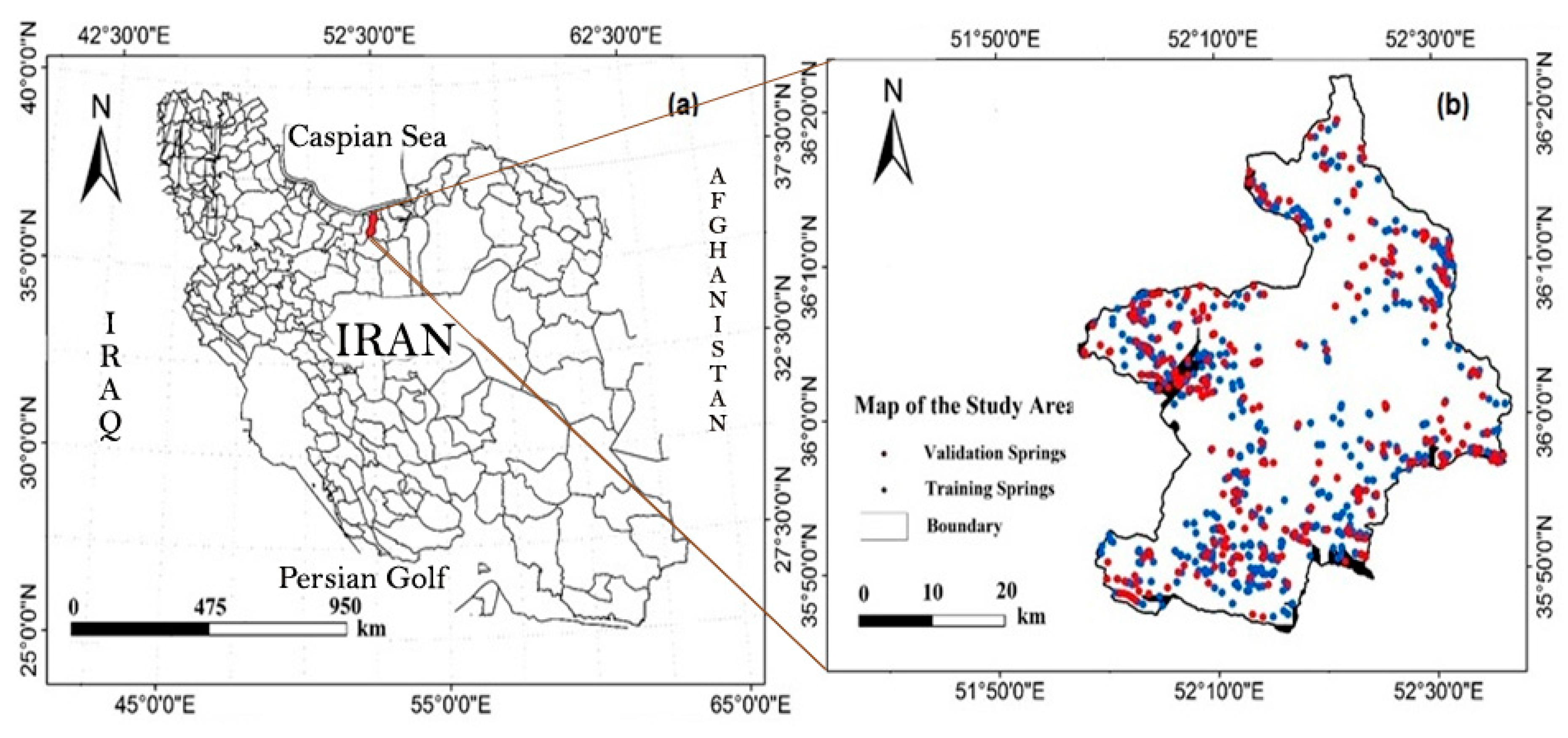
2. Study Area and Data Used

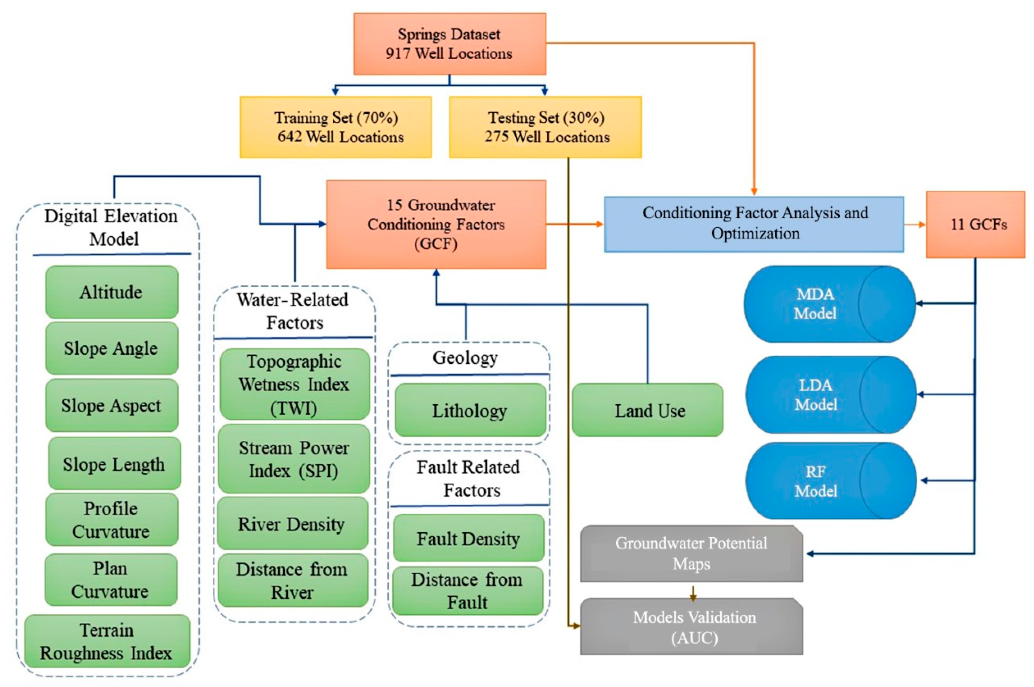
A representative subset of the Haraz basin in Mazandaran, Iran, is selected for this study. This basin is geographically located between longitudes of 51°56′ E to 52°36′ E and latitudes of 35°45′ N to 35°22′ N (Figure 1). It covers an area of 200,051-hectares, with altitude ranging between 200 m and 5600 m above mean sea level. The lithology of the Haraz basin is shown in

Table 1. Lithology characteristics of the Haraz watershed, adapted from [35].

Group	Lithology	Formation	Symbol
A	Scree	-	$Q^{sc}$
	Young terraces	-	$Q_2^r$
	Old terraces	-	$Q_1^r$
	Agglomerate	-	$Q^{ag}$
	Trachy andesitic lava flow	-	$Q^{ta}$
	Ash tuff, lapilli tuff	-	$Q^{ta}$
	Olivine basalt	-	$Q^b$
B	Green tuff, basaltic and limestone with gypsum, and conglomerate	Karaj	$K_K^{IV}$
C	Gypsum	Karaj	$E_K^{gy}$
	Limestone bearing nummulites and alveolina, conglomerate	Ziarat	$P{E}_z$
	Conglomerate, agglomerate, some marl, and limestone	Fajan	$P{E}_r$
D	Biogenic and cherty limestone	-	$K_2$
	Orbitoline bearing limestone	Tizkuh	$K_1$
	Massive to well-bedded, cherty limestone	Lar	$J_1$
	Well-bedded, partly oolitic-detritic limestone, marlylimestone	Dalichai	$J_d$
E	Dark shale and sandstone with plant remains, coal	Shemshak	$J_s$
	Thin-bedded limestone	Elika	$T{R}_{el}$
	Cross-bedded, quartzitic sandstone	Dorud	$P_d$

; the lithology map was produced by the Geological Survey of Iran (GSI) at a scale of 1:50,000. Apparently, the presence of limestone (Figure 2) increases the rate of groundwater incidence [33]. Within the basin, using Landsat Enhanced Thematic Mapper (2017) images, grassland (rangeland) makes up a majority of the land cover type, taking up approximately 152,625-hectares. Other land use types, namely farm, forest, garden, village, rock, and trees also make up approximately 47,426-hectares of the entire land cover. The temperature varies between −6.28 °C in the winter to 50 °C in the summer. According to the Iranian Meteorological Department, mean annual rainfall varies from 202 mm to 1,069 mm per annum, occurring between November and January [34]. A 20-m resolution digital elevation model (DEM) was created from a 1:25,000-scale topographic map of the Haraz basin. Evidently, wells, springs, rivers, etc. are the point of discharge for groundwater from the aquifer layer [2,17]; hence, in this study, spring locations are identified as the groundwater resource indicators. An inventory map from comprehensive field surveys by the Iranian Department of Water Resource Management, Iran (Figure 1), pinpoints the locations of 917 springs.

3. Data Preparation

We used groundwater inventory map as our dataset. Overall, 917 springs locations were randomly split into 70% for training and 30% for validation of the models, based on previous studies [26,36,37]. Initially, based on the literature in [20,33,38,39], site conditions, and data availability, 15 GCFs were considered for modeling, namely:

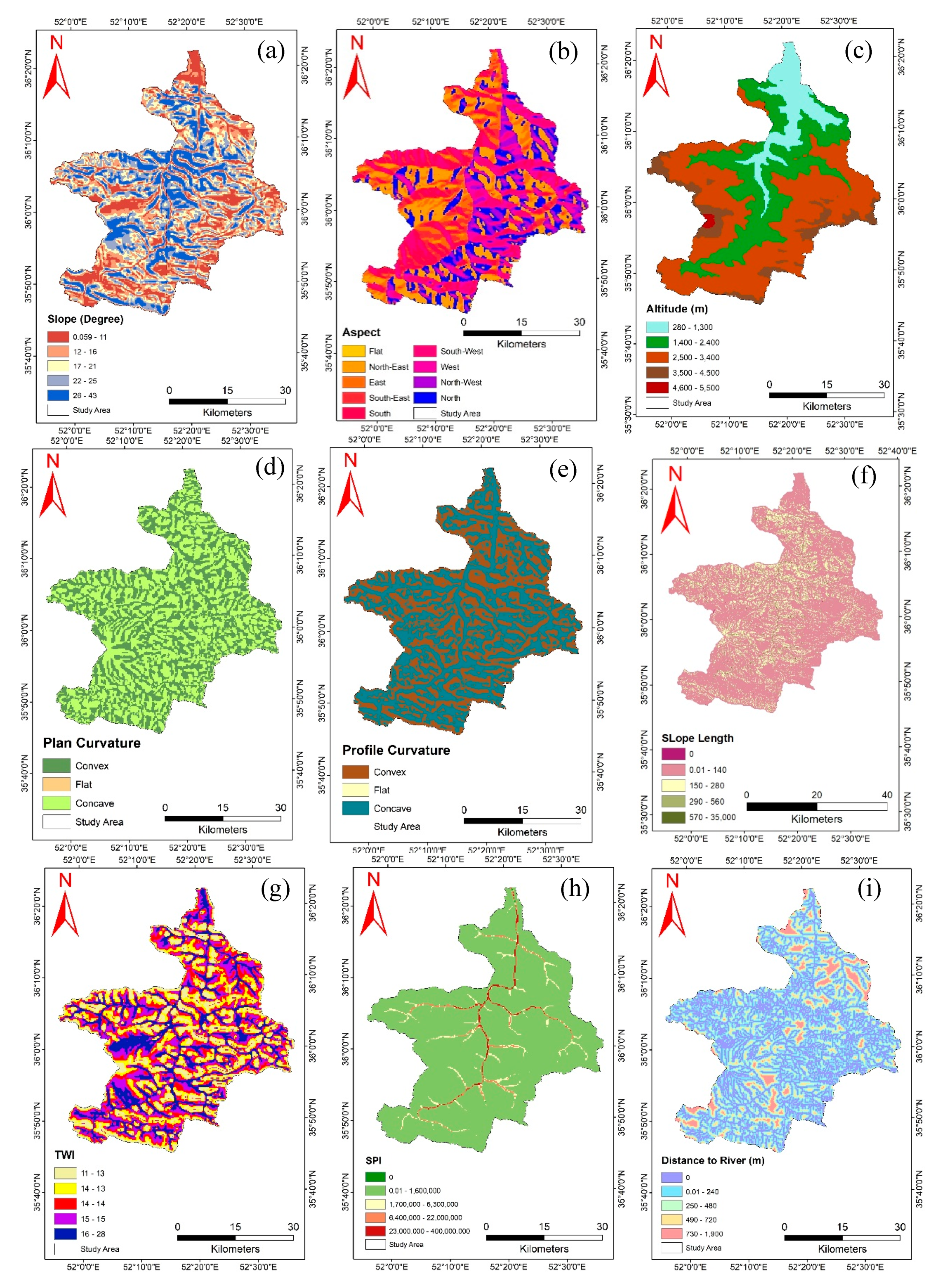
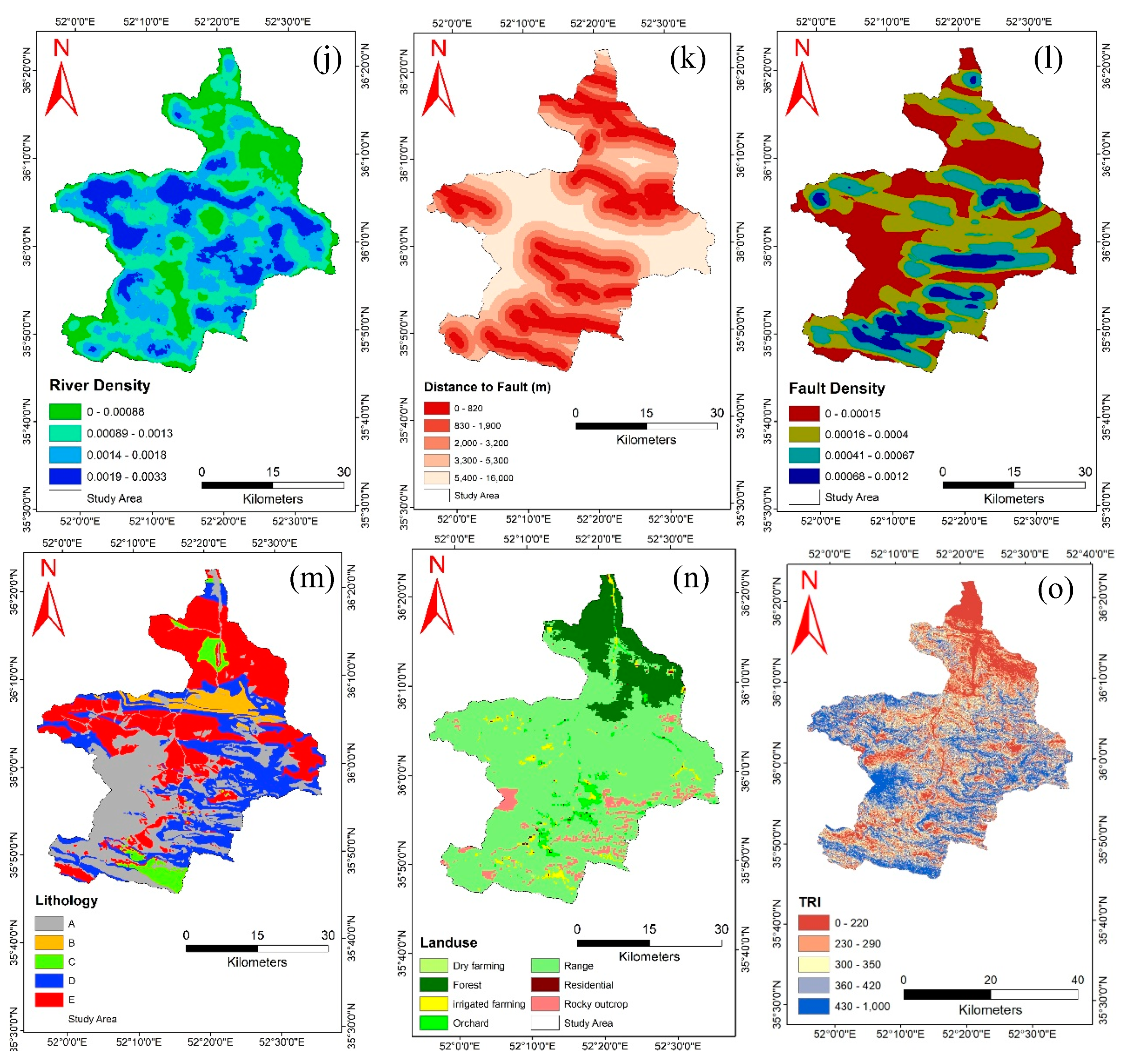
• Six elevation elements (slope angle, aspect angle, altitude, profile curvature, plan curvature, slope length);
• Five water-related factors (river density, distance from river, stream power index (SPI), terrain roughness index (TRI), and topographic wetness index (TWI));
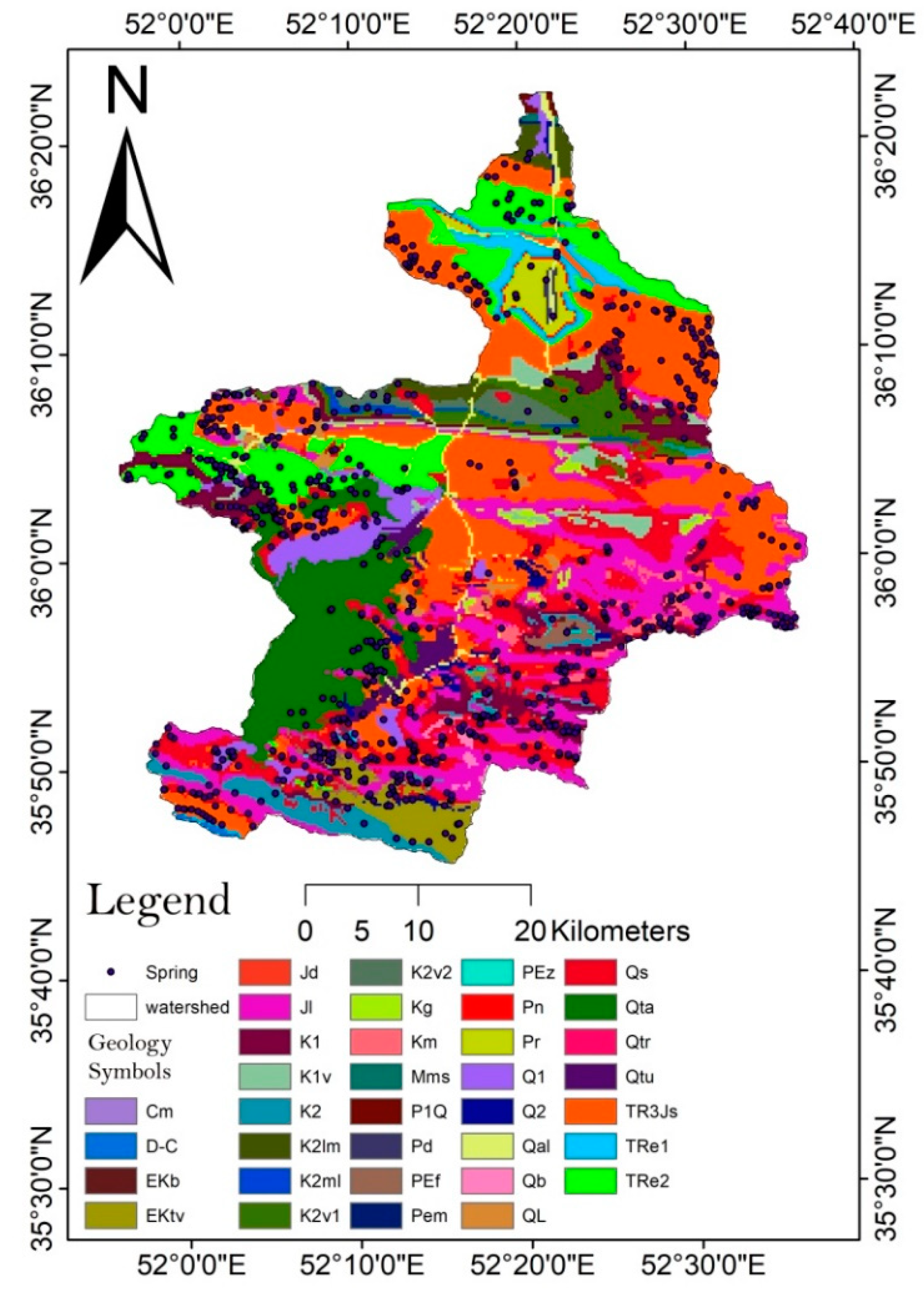
• Three geological factors (lithology, fault density, and distance from fault);
• Land use data, as illustrated in Figure 3.

Specifically, the six topographic conditioning factors were derived from the 20-m resolution DEM exploited from a 1:25,000-scale topographic map. The slope angle, as an effective regional hydraulic behavior [38], was reclassified into five classes (0°–11°, 12°–16°, 17°–21°, 22°–25° and 26°–43°) using the quantile classification scheme presented by [19], which is visualized in Figure 3a. Then, the slope aspect (Figure 3b) was classified into the 9 classes of (i) northeast, (ii) southeast, (iii) east, (iv) south, (v) west, (vi) southwest, (vii) north, (viii) northwest, and (ix) flat, based on normal and standard classification [40]. The slope aspect is related to two factors, namely, frontal precipitation direction and physiographic trends, which could influence weathering processes, growing vegetation, and recharging of groundwater [27,38]. The elevation map in Figure 3c shows the five elevation classes i.e., 280–1300 m, 1400–2400 m, 2500–3400 m, 3500–4500 m, and 4600–5500 m, using the equal-interval scheme [41]. In addition, we used ArcGIS to extract the Plan and Profile curvatures, which were then classified into three classes: (i) convex (positive curvature), (ii) flat (zero), and (iii) concave (negative curvature). These are shown in Figure 3d,e, which are adaptations from [42]. The slope-length (Figure 3f) was obtained from a combination of the slope steepness and slope length (L), as defined by [43] in Equation (1):

$$\mathrm{LS}={\left(\frac{Is}{22.13}\right)}^{0.6}{\left(\frac{\sin \alpha }{0.0896}\right)}^{1.3}$$

(1)

where $Is$ is the specific watershed area and $\alpha$ the slope gradient (measured in degrees).

Thereafter, the four water-related factors of river density, distance from the river, SPI and TWI are generated. The SPI is calculated using Equation (2), showing the amount of erosion power of flowing water, maintaining the assumption by [44], where discharge is relative to specific catchment area:

$$SPI= \lambda \times \tan \eta$$

(2)

In Equation (2), $\eta$ is the estimated local slope gradient (measured in degrees) and $\lambda$ is the specific catchment area.

TWI, on the other hand, is a factor indicating the spatial soil moisture pattern [43] and is calculated as in Equation (3):

$$TWI=In\left(\frac{\beta }{\tan \alpha }\right)$$

(3)

where $\beta$ is the cumulative upslope area draining through a particular point (per unit contour length) and $\tan \alpha$ represents the slope’s angle at that point. Classification of the TWI and SPI (Figure 3g,h) are achieved using the quantile classification scheme [19]. Distance from rivers is measured using the Euclidean distance and is calculated by ArcGIS 10.3. This distance was classified into five groups (Figure 3i) using the quantile classification scheme. The river density factor shown in Figure 3j was generated using line density functions and subsequently classified into four categories based on the natural break classification scheme [42].The terrain roughness index (TRI), or topographic roughness, is calculated by the sum of change in elevation between a grid cell and its neighborhood. The intuition behind this factor is that lower roughness values indicate higher spring potential mapping [20]. TRI is a geomorphometric parameter used to describe and quantify hills and valleys in the study area [45].

For geologic elements, the map of distance from faults is calculated using a geological map, and then classified into five classes (as per [19]) based on equal interval (Figure 3k). The fault density map (Figure 3l) was also classified into four classes using the natural break method [42]. Table 1 further shows the various types of lithological formations (A, B, C, D, and E) that cover the study area, which is consistent with [35]. This is further classified into five classes (Figure 3m). The Landsat Enhanced Thematic Mapper (2017) image is used to produce a land use map, which comprises of grasslands (rangeland), farms, forests, gardens, villages, rocks, and trees (Figure 3n). The maximum likelihood supervised classification scheme produced 88% overall classification accuracy.

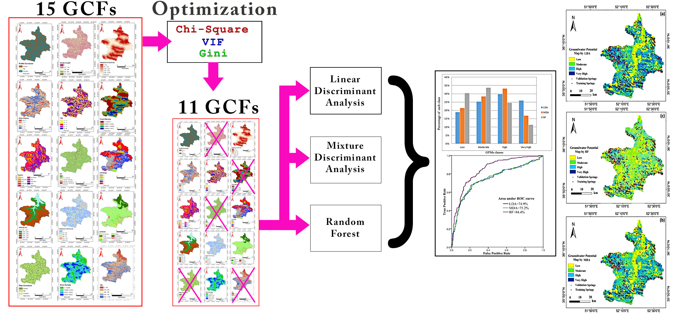
3.1. Groundwater Conditioning Factor Analysis and Optimization

Assessment of the various GCFs is essential to effectively determining accurate groundwater mapping. The author of [19] stated issues of multicollinearity, outliers, and spatial variations of conditioning factors, therefore necessitating factor analysis in assessment. This type of analysis allows redundant factors to be removed from the dataset for better model training and performance. Multicollinearity analysis stands for the existence of non-independence of GCFs in datasets due to their high correlation [40]. This implies that one predictor variable can be predicted considerably accurately, from other variables within a regression model. Here, we briefly summarize the three statistical factor analysis methods that have been exploited in this research.

3.1.1. Variance Inflation Factor (VIF)

VIF is the ratio of a model variance with multiple terms, divided by the model variance with one term [46]. It provides an index to indicate the increase of VIF due to collinearity. We examine all 15 GCFs against the VIF and Tolerance (or multicollinearity analysis) to observe any correlation between the 15 factors. Characteristically, according to [47], VIFs greater than 5 or 10 and tolerances less than 0.1 indicate multicollinearity.

3.1.2. Chi-Square Factor Optimization

In addition to factor optimization, another technique to detect redundancy is Chi-Square Factor Optimization, which calculates the significance of the relationship between conditioning factors [19]. In this work, a higher Chi-square value is responsible for a more important prediction factor to detect springs, where the p-value is evaluated against the significance level of 0.05. This allows to determine the significance relationship between GCF and the spring’s occurrences.

3.1.3. Gini Importance

The Gini coefficient is a summary statistic of the Lorenz curve and a measure of inequality in a population and the Statistical Information Value (IV), indicating the overall predictive power of the characteristics [19]. The IV is interpreted as follows: “Useless for prediction”—if the IV is less than 0.02; “Weak predictor” for IVs between 0.02 and 0.1; “Medium predictor” for IVs between 0.1 and 0.3, “Strong predictor” for IVs between 0.3 and 0.5; and “Suspicious or Too Good to be True” when IVs are greater than 0.5. Also, the Gini coefficient and Cramer’s V statistic (both ranging from 0 to 1) were computed for each factor. In the case of Gini coefficient, 0 indicates that all the variables are equal, while 1 denotes inequality among the variables. In contrast, Cramér’s V (based on Pearson’s Chi-squared statistic) measures the correlation between GCFs [19]. Here, 0 implies no correlation, whereas 1 shows a perfect correlation. Therefore, the highest value of Cramer’s V reveals the highest correlation between the factors, while the highest value of the Gini coefficient represents a lower correlation.

4. Methodology

The methodological workflow is presented in Figure 4. The corresponding pixel values of the 15 GCFs were extracted into the spring location points in ArcGIS 9.3, which was then imported into our R 3.0.2 (an open source software) implementation. These served as training and validation data for the principal and confirmatory models (RF, LDA, and MDA). Subsequently, the coefficients of the GCFs were calculated, and the values were converted into text format for statistical analysis and optimization (i.e., Variance Inflation Factor, Chi-Square Factor Optimization, and Gini Importance) using SPSS. Then, based on the analysis and optimization results, the most frequent factors (labeled as “least important”, or “multicollinearity factor” by the optimizers), were discarded. In the end, 11 final GCFs were used as input into the MDA, LDA, and RF algorithms. The database format was used to create the groundwater potential maps in ArcGIS. Lastly, the performance of the three models was evaluated.

4.1. Modeling Process

In this research, three supervised machine learning models (LD, MDA, and RF) were employed to produce GPMs. A brief explanation of each model is given in the following sections.

4.1.1. Linear Discriminant Analysis (LDA)

In the context of this work, LDA [48] is used to discover a linear combination of explanatory variables (or features) in order to perform classification, which can be seen as an attempt to estimate/predict a categorical dependent variable from explanatory variables. To achieve linearly separability, LDA assumes the following: (i) each of the categories has a multivariate normal distribution and (ii) each of the categories has the same covariance matrix.

LDA builds $j=min\left(k-1,p\right)$ discriminant functions (with $k$ equals the number of classes) to estimate the scores $D_{ji}$ for each of $i=1,\dots ,n$ instance. These instances will then be classified into one of the $k$ classes from the total of $p$ independent variables (commonly denoted using $X$). Specifically:

$$\begin{gathered} D_{ji}=w_{i1}{X}_{1i}+w_{i2}{X}_{2i}+\cdots +w_{ip}{X}_{pi} \\ \left[i = 1,\dots ,n and j = 1,\dots ,min\left(k-1,p\right)\right] \end{gathered}$$

(4)

The coefficients $w_{ij}$ (also termed as discriminant weights) can be reliably estimated using ordinary least squares. This is done to minimize the ratios’ inter- and intraclass variances between the $k$ classes. Resultantly, the function used for classification can be written as:

$$C_{ji}=c_{j0}+c_{j1}{X}_{1i}+c_{j2}{X}_{2i} + \dots +c_{jp}{X}_{pi}$$

(5)

In our work, the LDA model was constructed using the MASS package available in R 3.0.2.

4.1.2. Mixture Discriminant Analysis (MDA)

MDA is a classification technique first proposed by Hastie and Tibshirani [32]. In MDA, Gaussian mixtures are used for density estimation for each of the classes. Classically, the EM (expectation maximization) algorithm estimates the parameters and decides the number of components. This can also be seen as modeling multivariate intraclass densities of the predictors through a weighted sum of multivariate Gaussian distributions. This enables local fits to be obtained for each class by a mixture of Gaussians. MDA basically limits the intraclass spread of the subclass from the centers, relative to the interclass spread of multiple Gaussian distributions within one class [28]. This technique is applicable for either: (i) modeling multivariate non-normality or nonlinear relationships among variables within the respective group, in order to improve classification accuracy or (ii) to determine if hidden subclasses are present in each group [49]. In comparison with LDA, due to these multifunctional capabilities and MDA’s capability to smooth the decision boundaries and perform regularization [32], MDA was selected for groundwater mapping in this study.

As a non-parametric classification method, MDA is expected to perform well for complex relationships [28]. The class densities of the predictors $P(X|G)$ is modeled using a Gaussian mixture model [32]. Assuming $J$ classes, the number of subclasses in each class can be represented by $R_j, \mathrm{where} j = 1, 2, \dots , J.$ The mixture density for class $R_j$ can hence be written as:

$$m_j\left(x\right)=P\left(X=x|G=j\right)={\left|2\pi {{\displaystyle \sum }}^{\text{}}j\right|}^{-1/2} {\displaystyle \sum }_{r=1}^{R_j}{\pi }_{jr}\exp \left\{-D\left(x, {\mu }_{jr}\right)/2\right\}$$

(6)

where $D\left(x, {\mu }_{jr}\right)$ is defined as:

$$D\left(x, {\mu }_{jr}\right)={\left(x-{\mu }_{jr}\right)}^T {\displaystyle \sum }_j^{-1}\left(x-{\mu }_{jr}\right)$$

(7)

with $X$ being a vector of measurements (e.g., values of the conditioning factors), $G$ the class of a given object (e.g., in this case 2), ${\displaystyle \sum }j$ the covariance matrix assumed common to the mixture sub-classes of the class $j$, and $\pi$_jr and µ_jr are the mixing probability and mean of the $r$-th subclass of the $j$-th class [30]. More details about the fundamental of MDA are extensively presented in [30,32].

4.1.3. Random Forest (RF) Model

RF falls under the umbrella of ensemble classifiers. Basically, a large number of decision trees are constructed on the basis of randomly bootstrapped training data [50]. In RF, a number of trees are selected and combined to make predictions [51]. During modeling and in the context of this work, each tree split is based on a random subset of the conditioning factors. The final model is the average of the results of all the trees [6]. From the dataset, random training sets are selected for modeling, and the predicted value is defined by evaluating the influence of all the generated trees [50]. The evaluation considers event occurrences or non-occurrences [52]. Two crucial indices exist: (i) the mean decrease accuracy and (ii) the Gini index [33]. According to the author of [53], any dataset not included in the modeling is referred to as OOB (out of bag). RF predicts variable importance by evaluating increases in prediction error upon permutation of the OOB data with all other variables unchanged, as indicated by [54]. The two parameters required for RF are: (i) the number of trees ($ntree$) and the number of variables ($mtry$). Specifically:

• $ntree$ is the total trees that need to be grown. More trees will theoretically end up with more stable models and covariate importance estimates. The tradeoff is both a higher memory and computing time. For datasets that are small, 50 trees, for example, may suffice. However, larger datasets might require 500 or more trees. Typically, $ntree$ $\ge 100$ might not have a significant impact on the results. In this work, we set $ntree=100$ as a conservative number.
• $mtry$ refers to the number of available variables for splitting at each tree node. The specific values for $mtry$ differ across the literature. For example, the author of [55] reported that different $mtry$ values have little impact on classification accuracy as well as other metrics such as sensitivity, specificity, kappa, and ROC. Conversely, the author of [56] asserts that a specific value of $mtry$ is important and greatly influences predictor performance. Due to conflicting evidence, we determined $mtry$ through a validation dataset. Specifically, we randomly selected 70% of the dataset to calibrate the random forest model. The remainder (30%) was used for validation, i.e., for accuracy testing. Effectively, we were after an value that minimizes the mean squared error (MSE) in the validation dataset.

The importance of the RF variable is computed for variable $Y_i$ with reference to OOB [51]. Variable importance $Y_i$ is obtained from:

$$VImp\left(Y_j\right)=\frac{1}{N}{{\displaystyle \sum }}_{t}errOO{B}_t^j-errOO{B}_t$$

(8)

In Equation (8), $N$ is the total number of trees. The function $VImp\left(Y_j\right)$ indicates the importance of the $j^{th}$ variable. The term $errOO{B}_t$ is the prediction error when all factors are considered, whereas $errOO{B}_t^j$ is the error after removing the $j^{th}$ variable.

RF defines the importance of each GCF based on the impact of the overall error on the model, where higher impact indicates higher importance [33]. RF has the ability to accommodate different types of variables and missing values by fitting the interactions between the predictors [57]. Among the benefits of using this algorithm are: (i) overfitting can be avoided, (ii) low bias and variance (since everything averages over many trees), (iii) low correlation of individual trees due to the vast diversity of the forests and using a limited number of factors, and (iv) robust error estimates [6]. This study implements RF using R (caret and C50 packages for C5.0 algorithm) to model groundwater. The default value of this parameter depends on which R package is used. The LD and MDA models were done in MASS and MDA package release R 3.0.2.

4.2. Accuracy Assessment

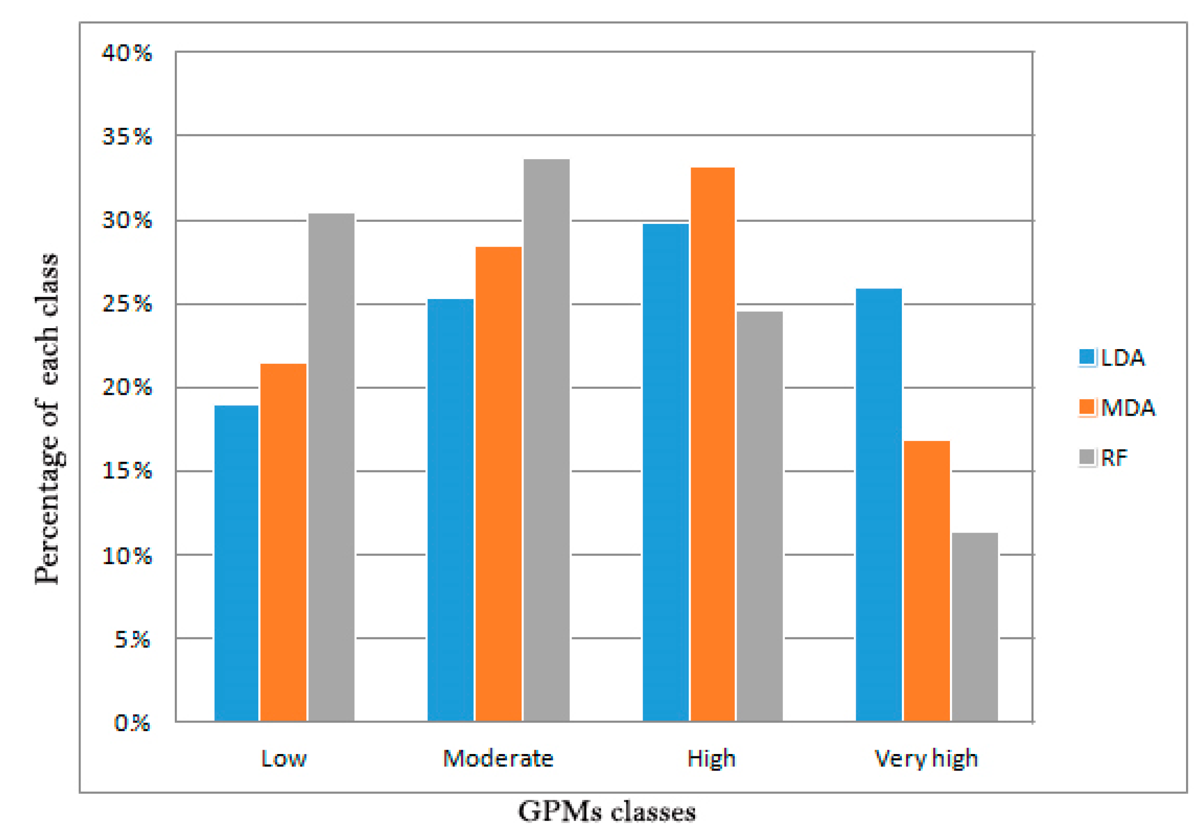
The Receiver Operating Characteristics (ROC) curve [58] is mainly used for assessing accuracy. It has been widely used in works involving land cover change, disease risk and species distribution studies [59], landslide susceptibility mapping [19,60], groundwater potential mapping [6], and for assessing groundwater vulnerability [61]. In this work, ROC assesses the spatial coincidence between the true event and predicts the probability of the model [59]. The ROC curve provides a quantitative assessment that is able to determine the uncertainty in modeling. It also takes into account biases associated with the estimation [42]. ROC analysis evaluates the effectiveness of spatial models that produce “probability” maps [59]. The ROC plots the true positive rate (TPR) vs. the false positive rate (FPR). True positives are when the model correctly classifies springs as springs, whereas false positives are when the actual label is a non-spring but falsely gets classified as a spring. The area under the ROC curve (commonly abbreviated as AUC) closer to 1 indicates better overall classification performance [33,62,63].

5. Results

For this research, the effectiveness of 15 GCFs was examined against VIF, Chi-square, and Gini importance methods. For the analysis, the two indices of VIF and tolerance were computed for GCFs (

Table 2. Estimated VIF for each groundwater conditioning factor (multicollinearity). (VIFs greater than 5 or 10 or tolerance less than 0.1 indicate multicollinearity).

Variable	Tolerance	VIF
Slope Length	0.2023	1.0427
Slope	0.9107	5.8622
SPI	0.0820	1.0068
TRI	0.9343	7.8669
River Density	0.1855	1.0356
TWI	0.3886	1.1779
Plan Curvature	0.3185	1.1129
Profile Curvature	0.1060	1.0114
Aspect	0.0253	1.0006
Altitude	0.8156	2.9876
Distance from Fault	0.2764	1.0827
Lithology	0.0338	1.0011
Land cover	0.2126	1.0473
Distance from River	0.2289	1.0553
Fault Density	0.2286	1.0551

), and it was observed that there was a correlation between TRI and slope angle as a result of the high VIF value; therefore, one of them is a redundant factor. Besides, SPI, slope aspect, and lithology’s tolerance values were found to be multi-collinear. To find out more, the Chi-square value and the p-value for each groundwater conditioning factor were calculated; the results of the factor optimization analysis are shown in

Table 3. Estimated factor importance and ranking using the Chi-square and Gini method.

Factor	Chi-Square Method		Gini Importance
	Chi-Square	p-Value	Gini	Information Value (IV)	Cramer’s V (Coefficient)
Distance from River	331.680	0.000	0.431	0.582	0.372
Land Cover	221.008	0.000	0.457	0.355	0.293
Altitude	116.349	0.000	0.474	0.214	0.227
Lithology	99.515	0.000	0.472	0.232	0.237
Slope	82.179	0.000	0.478	0.176	0.208
TWI	64.824	0.000	0.486	0.114	0.167
River Density	64.064	0.000	0.483	0.138	0.183
Profile Curvature	45.436	0.000	0.480	0.161	0.199
TRI	31.388	0.000	0.494	0.053	0.114
Fault Density	25.061	0.000	0.483	0.112	0.182
Distance from Fault	24.775	0.001	0.482	0.079	0.191
Aspect	6.189	0.518	0.496	0.032	0.090
Slope Length	6.126	0.409	0.497	0.020	0.071
SPI	3.145	0.534	0.495	0.040	0.099
Plan Curvature	1.001	0.317	0.488	0.096	0.154

. Based on the Chi-square analysis and p-value, the most important factors for GPMs were: distance from the river, land cover, altitude, and lithology. Note that plan curvature, SPI, slope length, and aspect were assigned as the least important factors.

Using Gini importance, IV value for distance from rivers was higher than 0.5, which indicates that this factor was a “Suspicious” or “Too Good to be True” predictor. Additionally, IV for land cover factor was calculated to be between 0.3 and 0.5, which indicates it to be a “Strong” predictor. Altitude, slope, and lithology factors were labeled as “Medium” predictor. Finally, the “Useless” predictor went to slope length; and other factors were labeled as “Weak” predictors. In view of all these optimization and factor analysis results, the common points are summarized as follows:

• Slope aspect, slope length, SPI, and TRI were the least important conditioning factors for GPMs, while distance from the river, land cover, altitude, and lithology were the most important factors.
• A slight correlation was confirmed by Gini coefficient (all value less than 0.5) and Cramer’s V (all values less than 0.37) for all factors.

Eventually, we observed that slope angle was tagged as a “Medium” predictor by IV; hence, the correlation between slope angle and TRI in VIF resulted in keeping slope and eliminating TRI from the conditioning factors. With a view on subsequent stages, we removed the redundant factors and finalized 11 conditioning factors—altitude, slope angle, plan curvature, profile curvature, topographic wetness index (TWI), distance from river, distance from fault, river density, fault density, land use, and lithology.

In this section, we show how implementation of LDA, MDA, and RF produce potential mappings for groundwater zones. The zones are categorized into four levels of potentiality—Very-High (0.75–1.00), High (0.5–0.75), Moderate (0.25–0.5), and Low (0–0.25)—using natural break (Figure 5a–c, respectively). To train each model, we used 642 from the total of 917 spring locations from our dataset. It is worth noting that the results obtained were based on the best average accuracy for each classifier using 10-fold cross validation (TFCV) based on a 70–30% training-test split. Briefly, TFCV (which is a specific implementation of $\mathrm{k}$-fold cross validation) partitions our dataset into 10-partitions. In the first fold, seven partitions of the data are used to train each model, whereas three partitions are used for testing. The accuracy at this fold is then calculated and recorded. This is followed by using a different 70–30% combination of the data for training and testing, respectively, whose accuracy is also calculated and recorded. In the end, after all 10-folds have been exhausted, overall average accuracy is calculated. The main justification for adopting TFCV is so that can ultimately determine the classifier with the highest average accuracy. Accuracy results based on cross validation is touted to be a better evaluation reference with regards to average predictive performance, especially if performing classifier selection [64]. Hence, cross validation can be said to be advantageous as compared to, say, a one-off 70–30% training-test split.

By analyzing the benchmark models in Figure 6, RF indicates that 11.32% of the entire area represents Very High potential, 24% High, 33.65% Moderate, and 30.45% Low. LDA, on the other hand, classifies 29.76% of the site as “High” potential, with 18.97% as “Low”. MDA’s results mapped 33.14% of the area as “High” potential, and 16.88% as “Very High”. Among the four classes, “Very High” and “Low” produced different values within predicted zones for the three models. MDA and RF seem more correlated than LDA in terms of class percentage. In general, a majority of the area is of “Moderate” and “High” groundwater potential. “Low” and “Very High” categories are lower in overall percentages coverage (Figure 5a,b and Figure 6).

As earlier mentioned, the models were validated using the ROC curve. AUC values of 1 show a perfect prediction of the models and indicate that highly ranked probabilities coincide with the spring’s locations [59]. In our analysis, the predicted groundwater potential maps were examined and compared with the inventory map of spring locations to evaluate the spatial coincidence between the probable values (from GPMs) and the real event (from springs map). Hence, 275 absolute spring locations (30% of the springs from inventory map) were examined against 275 randomly selected points from GPMs, showing no springs from the “Low” potential zone. The performances of each model are shown in Figure 7. Based on the performance evaluation, RF yields area a value of 84.4% under the ROC curve, which is better than the MDA and LDA models with 75.2% and 74.9%, respectively.

6. Discussion

The results of VIF, Chi-square, and Gini importance demonstrate that sole reliance on VIF is useless for factor optimization. In order to identify the important factors that need to be selected (and which ones should be discarded), further analysis is required. Moreover, highlighting distance from the river, land cover, DEM and lithology as significant factors are consistent with another study by [40]. However, the author of [40] mentioned that previous studies showed other conditioning factors as the most/least important factors for GPMs; among them, altitude was the more highly ranked factor and this diversity could be the result of different hydro-geological, climatic, and topographical features of the watersheds. However, the result of our factor analysis appeared to suggest that parameters such as aspect, slope length, TRI, and SPI do not have a significant contribution to the estimated groundwater potential.

By looking at GPMs resulting from MDA and LDA (Figure 5a,b), the distribution of four probability classes and their patterns were nearly the same. For example, the “Low” and “Moderate” classes appeared north-south at the center of the basin, particularly within altitude ranging from 280 m to 2400 m above mean sea level. LDA and MDA GPMs indicate higher occurrences of “High” classes, which cover approximately 1/3 of the entire area. However, the results are different for RF (Figure 5c), where the “Low” and “Moderate” classes were dominant. For instance, distribution of potential springs was classified as “Low” and “Moderate” in the west-south area, where the altitudes vary between 2800 m and 3300 m (the area involved no fault, it was steep, and lithologically it was covered by volcanic tuff). This pattern was followed by areas with lower fault density (e.g., north-east and north). In the north-south direction, at the center of the basin, where the altitude was lower than 2000 m, the areas were moderately disposed to groundwater zones (moderate class).

Generally, lower altitudes include lesser slope areas with developed drainage systems. These could be the reasons for the observed inverse relationship between altitude and spring occurrences, which is also what was concluded by [40]. The absence of springs in excessive slopes may not mean that the springs do not exist. Instead, there is a possibility that they were not detected during field work in inaccessible areas, which was pointed out by the work in [59]. The two other classes, “High” and “Very-High”, were generally distributed all around the spring’s locations and close to the study area’s border, with concentrations of dark shale and sandstone, limestone, and quartzitic sandstone.

It is worth noting that the results can suffer from the presence of bias in both training and validation data, due to easier accessibility to lower altitude areas to create inventory maps [59]. Therefore, the data might underestimate the presence of the springs at higher elevation areas because of difficulty during the field surveying. Considering the slope angle of the study area, the absence of springs in very steep areas (higher than 30 degrees) was obvious. This may indicate the incompleteness in the spring inventory map and its effect on training and validation data.

With respect to fault density, lower densities seem to indicate smaller springs concentrations and subsequently, lower potential for groundwater recourses. Surprisingly, land cover factor that was statistically categorized as one of the perfect conditioning factors to delineate GPM, was not as high as expected as we did not observe any remarkable influence by any specific land cover type. Besides that, the author of [20] concluded that garden land cover is systematically promoted by the nearest distance to the springs locations; therefore, we could not consider land cover as an independent variable. To compare with the research done by [20], the authors used aspect, TRI, and SPI, along with 10 other GCFs, and obtained maximum AUC of 87.5% using adaptive neuro-fuzzy inference systems. They used VIF Collinearity statistics and concluded that there was no multicollinearity in the datasets and determined land cover/use as the most important factor using information gain ratio (IGR). They also emphasized the effect of aspect, TRI, and SPI in prediction models, whereas in our experiment, we did not observe much effect and could obtain satisfying results without aspect, TRI, and SPI. This may suggest that site conditions and GCFs play different roles in a particular study area. With respect to fault distance, it was confirmed that the nearer to the fault, the higher is the probability of spring occurrence.

In general, the presence of groundwater resources within the study area was promising. Our findings indicate that most of the springs were in “High” and “Very High” classes, which covered almost every part of the study area. In the present study, we compared Linear and Mixed Discriminant Analyses and RF for groundwater potential mapping. Generally, LDA and MDA are optimal for discriminant analysis, where MDA seems to be a clear choice. The results of previous research [26] on groundwater potential mapping using LDA in Beheshtabad Watershed, Iran, with 14 GCFs and 1,425 springs locations, have shown that LDA had AUC-ROC of 0.735 with true positive rate of 69.1 and false positive rate of 60.3. In a study done by the author of [21], LDA achieved an acceptable performance with AUC-ROC value of 79.2% for groundwater potential mapping in the Khalkhal region, Ardebil Province, Iran. They found that LDA provided more detailed information about the modeling process. The work in [30] however reported the opposite, where LDA generally resulted in poor accuracy; however, MDA achieves higher accuracy, but typically lacks interpretability. To investigate MDA performance, LDA and RF were selected because they had been used in groundwater potential mapping in previous studies and were proven to produce acceptable results. Additionally, MDA is an advanced version of LDA, and comparison of these models, which are from a branch of models, could result in useful outputs. Moreover, RF was benchmarked as a well-known, flexible [23], simple machine learning algorithm [6], and an efficient model [6,33] to compare our discriminate analysis performances with respect to groundwater potential mapping. The ROC further showed that all three models reached values greater than 70%, which confirm the acceptance of results for such modeling [33,39]. Based on this observation, the GPMs were perfectly coinciding with true events (spring’s locations); therefore, they are reliable for resource planning and monitoring. Moreover, the performance of the proposed MDA model against the reference models (RF and LDA) is also consistent with the work of [21]. Consequently, MDA seems to be a reliable approach for groundwater potential mapping. Although ROC-AUC is one of the most common indices to evaluate prediction models and was frequently used by [6,23,39,40,65,66,67,68] for groundwater potential mapping validation, our future research will further investigate the accuracy of MDA model for GPM using other validation methods. Moreover, we note, however, that the accuracy of the groundwater/springs inventory dataset has a significant effect on the validity and accuracy assessment of GPMs [37]. To improve accuracy, a variety of sources, such as field survey, remote sensing imagery, and aerial photos can be used to prepare a spring inventory map [68] and locate groundwater discharge [69], which can lead to a complete and accurate inventory map, even in inaccessible, steep, and high altitude areas.

7. Conclusions

Uncertainties in spatial modeling require the use of advanced modeling techniques in order to reduce the degree of uncertainty for reliable GPM. Various GCF datasets have been used for this research, such as geological, hydrological, topographical, lithological factors, and a land use map, together with a spring inventory map for training and accuracy assessment. Among these factors, distance from the river, land cover, and altitude were analyzed and defined to have more significant roles in GPMs. On the contrary, slope length, slope aspect, SPI, and TRI ranked as the least important factors. Moreover, ranking of factors shows small differences from one statistical factor analysis/optimization method to another. This is seen when lithology map was categorized as a good factor for modeling by Chi-square, while VIF and tolerance show a correlation with other factors. Hence, along with VIF, other factor analysis methods such as Chi-square or Gini importance can be utilized as well. The findings of our visual inspection also showed that fault density is one of the important conditioning factors for GPMs. We, however, did not observe direct impact of any specific land cover in GPMs, which was a theme mentioned by other researchers and our factor analysis. Based on all these observations, it may be suggested that the importance of any conditioning factor is subject to regional attributes and many other variables. Hence, factor ranking may vary from one study area to another. Consequently, we cannot rely on a single factor analysis method to remove redundant data. This study applied a relatively new model i.e. MDA, which was compared with two other models, namely, LDA and RF. The objective was to classify groundwater potential areas into four classes in the Haraz basin of Iran. Conclusively, RF produced a convincing ROC of 84.4%. This has informed its application as the baseline to evaluate the performance of LDA and MDA in this study. Obviously, the GPMs obtained with LDA and MDA prove that the two algorithms belong to the same family, as ROC analysis were closely related, and they showed a similar pattern in term of distribution of the potential classes, as well. As mentioned earlier, the result of this study verifies that RF’s is less affected by geographical attributes (rather than MDA and LDA). It also reveals the ability of RF to accommodate different types of variables as a prediction model. The apparent disparity in the distribution of the groundwater potential classes between the two mentioned discriminant algorithms and RF, which may arise from uncertainty in the modeling parameters or algorithm, needs further investigation. Further studies will be carried out to evaluate the performance of RF in different environments for groundwater potential mapping to verify its robustness under different conditioning parameters. Nevertheless, the results obtained from the models are resourceful for water resources managers to improve planning and management. The result of this research also suggests the use of complementary data to enrich springs inventory maps that directly affects the accuracy of GPM.

References

1. Bhat, T.A. An Analysis of Demand and Supply of Water in India. J. Environ. Earth Sci. 2014, 4, 67–72. [Google Scholar]
2. Manap, M.A.; Sulaiman, W.N.A.; Ramli, M.F.; Pradhan, B.; Surip, N. A knowledge-driven GIS modeling technique for groundwater potential mapping at the Upper Langat Basin, Malaysia. Arab. J. Geosci. 2013, 6, 1621–1637. [Google Scholar] [CrossRef]
3. Akinwumiju, A.S.; Olorunfemi, M.O.; Afolabi, O. GIS-based integrated groundwater potential assessment of Osun drainage basin, southwestern Nigeria. IFE J. Sci. 2016, 18, 147–168. [Google Scholar]
4. Madani, K. Water management in Iran: What is causing the looming crisis? J. Environ. Stud. Sci. 2014, 4, 315–328. [Google Scholar] [CrossRef]
5. Bastani, M.; Kholghi, M.; Rakhshandehroo, G.R. Inverse modeling of variable-density groundwater flow in a semi-arid area in Iran using a genetic algorithm. Hydrogeol. J. 2010, 18, 1191–1203. [Google Scholar] [CrossRef]
6. Rahmati, O.; Pourghasemi, H.R.; Melesse, A.M. Application of GIS-based data driven random forest and maximum entropy models for groundwater potential mapping: A case study at Mehran Region, Iran. Catena 2016, 137, 360–372. [Google Scholar] [CrossRef]
7. Sokeng, V.-C.J.; Kouame, F.; Nagatcha, N.; N’da, H.D.; You, L.A.; Rirabe, D. Delineating groundwater potential zones in Western Cameroon Highlands using GIS based Artificial Neural Networks model and remote sensing data. Int. J. Innov. Appl. Stud. 2016, 15, 747–759. [Google Scholar]
8. Díaz-Alcaide, S.; Martínez-Santos, P.; Villarroya, F. A commune-level groundwater potential map for the republic of Mali. Water 2017, 9, 839. [Google Scholar] [CrossRef]
9. Machiwal, D.; Jha, M.K.; Singh, P.K.; Mahnot, S.C.; Gupta, A. Planning and design of cost-effective water harvesting structures for efficient utilization of scarce water resources in semi-arid regions of Rajasthan, India. Water Resour. Manag. 2004, 18, 219–235. [Google Scholar] [CrossRef]
10. Sturm, M.; Zimmermann, M.; Schütz, K.; Urban, W.; Hartung, H. Rainwater harvesting as an alternative water resource in rural sites in central northern Namibia. Phys. Chem. Earth 2009, 34, 776–785. [Google Scholar] [CrossRef]
11. Wu, P.; Tan, M. Challenges for sustainable urbanization: A case study of water shortage and water environment changes in Shandong, China. Procedia Environ. Sci. 2012, 13, 919–927. [Google Scholar] [CrossRef]
12. Chowdhury, A.; Jha, M.K.; Chowdary, V.M.; Mal, B.C. Integrated remote sensing and GIS-based approach for assessing groundwater potential in West Medinipur district, West Bengal, India. Int. J. Remote Sens. 2008, 30, 231–250. [Google Scholar] [CrossRef]
13. Talabi, A.O. Weathering of Meta-Igneous Rocks in Parts of the Basement Terrain of Southwestern Nigeria: Implications on Groundwater Occurrence. Int. J. Sci. Res. Publ. 2015, 5, 1–17. [Google Scholar]
14. Deshpande, S.M.; Aher, K.R. Evaluation of Groundwater Quality and its Suitability for Drinking and Agriculture use in Parts of Vaijapur, District Aurangabad, MS, India. J. Chem. Sci. 2012, 2, 25–31. [Google Scholar]
15. Elbeih, S.F. An overview of integrated remote sensing and GIS for groundwater mapping in Egypt. Ain Shams Eng. J. 2014, 6, 1–15. [Google Scholar] [CrossRef]
16. Tahmassebipoor, N.; Rahmati, O.; Noormohamadi, F.; Lee, S. Spatial analysis of groundwater potential using weights-of-evidence and evidential belief function models and remote sensing. Arab. J. Geosci. 2016, 9, 1–18. [Google Scholar] [CrossRef]
17. Haghizadeh, A.; Moghaddam, D.D.; Pourghasemi, H.R. GIS-based bivariate statistical techniques for groundwater potential analysis (An example of Iran). J. Earth Syst. Sci. 2017, 126, 1–17. [Google Scholar] [CrossRef]
18. Marjani, M.; Nasaruddin, F.; Gani, A.; Karim, A.; Hashem, I.A.T.; Siddiqa, A.; Yaqoob, I. Big IoT Data Analytics: Architecture, Opportunities, and Open Research Challenges. IEEE Access 2017, 5, 5247–5261. [Google Scholar]
19. Pradhan, B.; Seeni, M.I.; Kalantar, B. Performance Evaluation and Sensitivity Analysis of Expert-Based, Statistical, Machine Learning, and Hybrid Models for Producing Landslide Susceptibility Maps. In Laser Scanning Applications in Landslide Assessment; Springer: Cham, Switzerland, 2017; pp. 193–232. ISBN 9783319553429. [Google Scholar]
20. Khosravi, K.; Panahi, M.; Tien Bui, D. Spatial prediction of groundwater spring potential mapping based on an adaptive neuro-fuzzy inference system and metaheuristic optimization. Hydrol. Earth Syst. Sci. 2018, 22, 4771–4792. [Google Scholar] [CrossRef] [Green Version]
21. Naghibi, S.A.; Moradi Dashtpagerdi, M. Evaluation of four supervised learning methods for groundwater spring potential mapping in Khalkhal region (Iran) using GIS-based featuresEvaluation de quatre méthodes d’apprentissage supervisé pour la cartographie du potentiel des sources d’eaux souterra. Hydrogeol. J. 2017, 25, 169–189. [Google Scholar] [CrossRef]
22. Close, M.E.; Abraham, P.; Humphries, B.; Lilburne, L.; Cuthill, T.; Wilson, S. Predicting groundwater redox status on a regional scale using linear discriminant analysis. J. Contam. Hydrol. 2016, 191, 19–32. [Google Scholar] [CrossRef] [PubMed]
23. Zabihi, M.; Pourghasemi, H.R.; Pourtaghi, Z.S.; Behzadfar, M. GIS-based multivariate adaptive regression spline and random forest models for groundwater potential mapping in Iran. Environ. Earth Sci. 2016, 75, 1–19. [Google Scholar] [CrossRef]
24. Lee, S.; Hong, S.M.; Jung, H.S. GIS-based groundwater potential mapping using artificial neural network and support vector machine models: The case of Boryeong city in Korea. Geocarto Int. 2018, 33, 847–861. [Google Scholar] [CrossRef]
25. Lee, S.; Lee, C.W. Application of decision-tree model to groundwater productivity-potential mapping. Sustainability 2015, 7, 13416–13432. [Google Scholar] [CrossRef]
26. Naghibi, S.A.; Pourghasemi, H.R.; Abbaspour, K. A comparison between ten advanced and soft computing models for groundwater qanat potential assessment in Iran using R and GIS. Theor. Appl. Climatol. 2018, 131, 967–984. [Google Scholar] [CrossRef]
27. Falah, F.; Ghorbani Nejad, S.; Rahmati, O.; Daneshfar, M.; Zeinivand, H. Applicability of generalized additive model in groundwater potential modelling and comparison its performance by bivariate statistical methods. Geocarto Int. 2017, 32, 1069–1089. [Google Scholar] [CrossRef]
28. Li, X.; Wang, Y. Applying various algorithms for species distribution modelling. Integr. Zool. 2013, 8, 124–135. [Google Scholar] [CrossRef] [PubMed]
29. Hoang, N.D.; Bui, D.T. Predicting earthquake-induced soil liquefaction based on a hybridization of kernel Fisher discriminant analysis and a least squares support vector machine: A multi-dataset study. Bull. Eng. Geol. Environ. 2018, 77, 191–204. [Google Scholar] [CrossRef]
30. Ju, J.; Kolaczyk, E.D.; Gopal, S. Gaussian mixture discriminant analysis and sub-pixel land cover characterization in remote sensing. Remote Sens. Environ. 2003, 84, 550–560. [Google Scholar] [CrossRef]
31. Lombardo, F.; Obach, R.S.; DiCapua, F.M.; Bakken, G.A.; Lu, J.; Potter, D.M.; Gao, F.; Miller, M.D.; Zhang, Y. A hybrid mixture discriminant analysis-random forest computational model for the prediction of volume of distribution of drugs in human. J. Med. Chem. 2006, 49, 2262–2267. [Google Scholar] [CrossRef]
32. Hastie, T.; Tibshirani, R. Discriminant Analysis by Gaussian Mixtures. J. R. Stat. Soc. Ser. B 1996, 58, 155–176. [Google Scholar] [CrossRef]
33. Hong, H.; Liu, J.; Zhu, A.X.; Shahabi, H.; Pham, B.T.; Chen, W.; Pradhan, B.; Tien Bui, D. A novel hybrid integration model using support vector machines and random subspace for weather-triggered landslide susceptibility assessment in the Wuning area (China). Environ. Earth. Sci. 2017, 76, 652. [Google Scholar] [CrossRef]
34. Abbaspour, K.C.; Faramarzi, M.; Ghasemi, S.S.; Yang, H. Assessing the impact of climate change on water resources in Iran. Water Resour. Res. 2009, 45, 1–16. [Google Scholar] [CrossRef]
35. Pourghasemi, H.R.; Pradhan, B.; Gokceoglu, C. Application of fuzzy logic and analytical hierarchy process (AHP) to landslide susceptibility mapping at Haraz watershed, Iran. Nat. Hazards 2012, 63, 965–996. [Google Scholar] [CrossRef]
36. Naghibi, S.A.; Dolatkordestani, M.; Rezaei, A.; Amouzegari, P.; Heravi, M.T.; Kalantar, B.; Pradhan, B. Application of rotation forest with decision trees as base classifier and a novel ensemble model in spatial modeling of groundwater potential. Environ. Monit. Assess. 2019, 191, 248. [Google Scholar] [CrossRef] [PubMed]
37. Golkarian, A.; Naghibi, S.A.; Kalantar, B.; Pradhan, B. Groundwater potential mapping using C5.0, random forest, and multivariate adaptive regression spline models in GIS. Environ. Monit. Assess. 2018, 190, 149. [Google Scholar] [CrossRef] [PubMed]
38. Daneshfar, M.; Zeinivand, H. Journal of Applied Hydrology. J. Appl. Hydrol. 2015, 2, 45–61. [Google Scholar]
39. Kordestani, M.D.; Naghibi, S.A.; Hashemi, H.; Ahmadi, K.; Kalantar, B.; Pradhan, B. Groundwater potential mapping using a novel data-mining ensemble model. Hydrogeol. J. 2019, 27, 211–224. [Google Scholar] [CrossRef]
40. Mousavi, S.M.; Golkarian, A.; Naghibi, S.A.; Kalantar, B.; Pradhan, B. GIS-based Groundwater Spring Potential Mapping Using Data Mining Boosted Regression Tree and Probabilistic Frequency Ratio Models in Iran. Aims Geosci. 2017, 3, 91–115. [Google Scholar]
41. Pourtaghi, Z.S.; Pourghasemi, H.R. Evaluation de la potentialité des sources d’eau souterraine à partir d’un SIG et cartographie dans le district de Birjand, Sud de la province de Khorasan, Iran. Hydrogeol. J. 2014, 22, 643–662. [Google Scholar] [CrossRef]
42. Zare, M.; Porghasemi, H.R.; Vafakhah, M.; Pradhan, B. Application of weights-of-evidence and certainty factor models and their comparison in landslide susceptibility mapping at Haraz watershed, Iran. Arab. J. Geosci. 2013, 6, 2873–2888. [Google Scholar] [CrossRef]
43. Moore, I.D.; Burch, G.J. Sediment transport capacity of sheet and rill flow' Application of unit stream power theory. Water Resour. Res. 1986, 22, 1350–1360. [Google Scholar] [CrossRef]
44. Moore, I.D.; Grayson, R.B. Terrain-based catchment partitioning and runoff prediction using vector elevation data. Water Resour. Res. 1991, 27, 1177–1191. [Google Scholar] [CrossRef]
45. Różycka, M.; Migoń, P.; Michniewicz, A. Topographic Wetness Index and Terrain Ruggedness Index in geomorphic characterisation of landslide terrains, on examples from the Sudetes, SW Poland. Z. Geomorphol. 2015, 59, 227–245. [Google Scholar] [CrossRef]
46. Dormann, C.F.; Elith, J.; Bacher, S.; Buchmann, C.; Carl, G.; Carré, G.; Marquéz, J.R.G.; Gruber, B.; Lafourcade, B.; Leitão, P.J.; et al. Collinearity: A review of methods to deal with it and a simulation study evaluating their performance. Ecography 2013, 36, 027–046. [Google Scholar] [CrossRef]
47. O’Brien, R.M. A caution regarding rules of thumb for variance inflation factors. Qual. Quant. 2007, 41, 673–690. [Google Scholar] [CrossRef]
48. Fisher, R.A. The Use of Multiple Measurements in Taxonomic Problems. Ann. Eugen. 1936, 7, 179–188. [Google Scholar] [CrossRef]
49. Rausch, J.R.; Kelley, K. A comparison of linear and mixture models for discriminant analysis under nonnormality. Behav. Res. Methods 2009, 41, 85–98. [Google Scholar] [CrossRef] [PubMed]
50. Breiman, L. Random forests. Mach. Learn. 2001, 45, 5–32. [Google Scholar] [CrossRef]
51. Van Beijma, S.; Comber, A.; Lamb, A. Random forest classification of salt marsh vegetation habitats using quad-polarimetric airborne SAR, elevation and optical RS data. Remote Sens. Environ. 2014, 149, 118–129. [Google Scholar] [CrossRef]
52. Immitzer, M.; Atzberger, C.; Koukal, T. Tree species classification with Random forest using very high spatial resolution 8-band worldView-2 satellite data. Remote Sens. 2012, 4, 2661–2693. [Google Scholar] [CrossRef]
53. Catani, F.; Lagomarsino, D.; Segoni, S.; Tofani, V. Landslide susceptibility estimation by random forests technique: Sensitivity and scaling issues. Nat. Hazards Earth Syst. Sci. 2013, 13, 2815–2831. [Google Scholar] [CrossRef]
54. Liaw, A.; Wiener, M. Classification and regression by randomForest. Forest 2002, 2, 18–22. [Google Scholar]
55. Cutler, R.; Lawler, J.; Thomas Edwards, J.; Beard, K.H.; Cutler, A.; Hess, K.T.; Gibson, J. Random Forests for Classification in Ecology. Ecology 2007, 88, 2783–2792. [Google Scholar] [CrossRef] [PubMed]
56. Strobl, C.; Boulesteix, A.L.; Kneib, T.; Augustin, T.; Zeileis, A. Conditional variable importance for random forests. BMC Bioinform. 2008, 9, 1–11. [Google Scholar] [CrossRef] [PubMed]
57. Pourghasemi, H.R.; Pradhan, B.; Gokceoglu, C.; Mohammadi, M.; Moradi, H.R. Application of weights-of-evidence and certainty factor models and their comparison in landslide susceptibility mapping at Haraz watershed, Iran. Arab. J. Geosci. 2013, 6, 2351–2365. [Google Scholar] [CrossRef]
58. Egan, J.P. Signal Detection Theory and ROC Analysis Academic Press Series in Cognition and Perception; Academic Press: New York, NY, USA, 1975. [Google Scholar]
59. Mas, J.-F.; Soares Filho, B.; Pontius, R.; Farfán Gutiérrez, M.; Rodrigues, H. A Suite of Tools for ROC Analysis of Spatial Models. ISPRS Int. J. Geo-Inf. 2013, 2, 869–887. [Google Scholar] [CrossRef]
60. Lee, S.; Lee, M.; Jung, H. applied sciences Data Mining Approaches for Landslide Susceptibility Mapping in Umyeonsan, Seoul, South Korea. Appl. Sci. 2017, 7, 683. [Google Scholar] [CrossRef]
61. Khosravi, K.; Sartaj, M.; Tsai, F.T.C.; Singh, V.P.; Kazakis, N.; Melesse, A.M.; Prakash, I.; Tien Bui, D.; Pham, B.T. A comparison study of DRASTIC methods with various objective methods for groundwater vulnerability assessment. Sci. Total Environ. 2018, 642, 1032–1049. [Google Scholar] [CrossRef] [PubMed]
62. Negnevitsky, M.; Pavlovsky, V. Neural networks approach to online identification of multiple failures of protection systems. IEEE Trans. Power Deliv. 2005, 20, 588–594. [Google Scholar] [CrossRef]
63. Bui, D.T.; Moayedi, H.; Kalantar, B.; Osouli, A.; Pradhan, B.; Nguyen, H.; Rashi, A.S.A. A Novel Swarm Intelligence—Harris Hawks. Sensors 2019, 19, 3590. [Google Scholar] [CrossRef] [PubMed]
64. Schaffer, C.; Schaffer, C. Selecting a Classification Method by Cross-Validation. Mach. Learn. 1993, 13, 135–143. [Google Scholar] [CrossRef]
65. Naghibi, S.A.; Moghaddam, D.D.; Kalantar, B.; Pradhan, B.; Kisi, O. A comparative assessment of GIS-based data mining models and a novel ensemble model in groundwater well potential mapping. J. Hydrol. 2017, 548, 471–483. [Google Scholar] [CrossRef]
66. Naghibi, S.A.; Pourghasemi, H.R. classification and regression tree, and random forest machine learning models in Iran GIS-based groundwater potential mapping using boosted regression tree, classification and regression tree, and random forest machine learning models in Iran. Environ. Monit. Assess. 2016, 188, 44. [Google Scholar] [CrossRef] [PubMed]
67. Pourtaghi, Z.S.; Pourghasemi, H.R. GIS-based groundwater spring potential assessment and mapping in the Birjand Township, southern Khorasan Province, Iran. Hydrogeol. J. 2014, 22, 643–662. [Google Scholar] [CrossRef]
68. Kalantar, B.; Pradhan, B.; Amir Naghibi, S.; Motevalli, A.; Mansor, S. Assessment of the effects of training data selection on the landslide susceptibility mapping: A comparison between support vector machine (SVM), logistic regression (LR) and artificial neural networks (ANN). Geomatics Nat. Hazards Risk 2018, 9, 49–69. [Google Scholar] [CrossRef]
69. Stefouli, M.; Vasileiou, E.; Charou, E.; Stathopoulos, N. Remote sensing techniques as a tool for detecting water outflows. Case Study Cephalonia Isl. 2013, 47, 1519. [Google Scholar]
Figure 1. Specific location of the study area on the Iranian map (a), and the spring map for training and validation (b).
Water 11 01909 g001
Figure 2. Lithology map of the study area (symbols were defined in Table 1).
Water 11 01909 g002
Figure 3. GCFs considered in this study: (a) slope angle, (b) slope aspect, (c) altitude, (d) plan curvature, (e) profile curvature, (f) slope length, (g) topographic wetness index, (h) stream power index, (i) distance from rivers, (j) river density, (k) distance from fault, (l) fault density, (m) lithology, (n) land use, and (o) terrain roughness index.
Water 11 01909 g003aWater 11 01909 g003b
Figure 4. Methodological flow chart.
Water 11 01909 g004
Figure 5. Groundwater potential map produced by (a) LDA, (b) MDA, and (c) RF models.
Water 11 01909 g005
Figure 6. The percentage of four predicted classes in GPMs derived from LDA, MDA and RF modeling.
Water 11 01909 g006
Figure 7. Receiver operating characteristics (ROC) curve calculated for the LDA, MDA and RF models.
Water 11 01909 g007