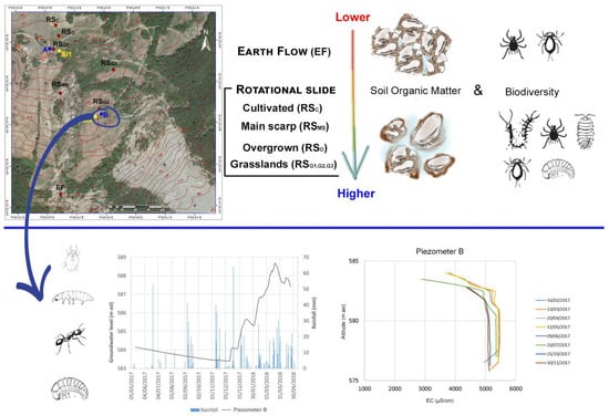
Hydrodynamic and Soil Biodiversity Characterization in an Active Landslide

Abstract

Landslides are common in the Northern Apennines (Italy) and their resulting changes in soil structure affect edaphic fauna biodiversity, whose activity has concurrent impacts on soil structural stability and water-holding capacity. The aim of this study was to characterise landslide evolution and assess potential relationships between its hydrogeological features and soil fauna. The landforms of the study area, located in the River Taro valley, were mapped and the hydraulic head fluctuations and groundwater electrical conductivity profiles were measured. The soil arthropod community was studied in seven sites, one subject to earth flow and six to rotational slide; the last ones were divided into the main scarp of the slide, and five sites characterized by different land use: three grassland, a wheat cultivated field and an overgrown area. Soil organic matter (SOM) and pH measurements were performed. Hydrogeological results suggest unexpected rapid percolation of relatively low-salinity waters through the unsaturated zone. Both lower SOM content and arthropod biodiversity were found in earth flow area, while higher values were found in grasslands. Fauna composition appears to be a good indicator of soil degradation processes, linked to the hydraulic features, and contributes to the evaluation of the soil condition in landslide areas for further agricultural purposes.

1. Introduction

Landslides are complex systems dependent on geological, geomorphological, hydrogeological and geotechnical factors, and represent worldwide danger for people, buildings and transportation infrastructures. They are common in the Northern Apennines (Italy), a folded and thrusted belt developed since the Cretaceous period [1,2,3,4], where different types of landslides can be detected and large earth flows are widespread [5]. In several areas, earth or rock rotational and/or translational slides evolve into earth flows [6,7]. These landslides can be huge [8], and the affected areas can reach up to 10⁵ m² (with displaced volumes up to 10⁸ m³).

A major role is played by tectonics, which caused the development of faults and thrusts (representing weak zones with associated sets of fractures) controlling the recent uplift that conditioned most of the slopes’ geomorphological evolution [6,9]. Nevertheless, rainfall is the triggering factor, especially during those seasons (usually, autumn and spring) that are characterised by precipitations lasting for several days [10]. The distribution of precipitation is influenced by the recent climate changes [11], and prolonged dry periods alternated with intense rainfalls are more and more frequent. The relationship between initial slope conditions and rainfall frequency/intensity, and the reactivation of large landslides is a major research challenge [12,13], and some authors have attempted to find one-to-one correlation between rainfalls thresholds and slope failures [14], or to integrate methods [15].

Above- and belowground biodiversity is affected by landslides: changes in site condition lead to changes in soil physical and chemical composition and, consequently, in vegetation cover, contributing to increased habitat diversity [16]. The most obvious consequences of landslides are on topography, yet these processes also have a substantial impact on soil properties, by exposing parent material and removing organic matter and A horizons that lead to textural and chemical changes. Landslide processes often bear textural sorting; moreover, remoulding and liquefaction of clays and silts in earth flows reduce structure and porosity, and increase soil density [17]. Changes in soil density and porosity are consequences of erosion, which leads to changes in soil chemistry too [17]. Soil organic matter is mostly found in the soil surface, therefore decreases significantly through erosion; formation of soil aggregates is consequently disrupted, and soil porosity decreases. Reduced soil organic matter leads to overall diminishing of biomass and productivity [18] and sets back the ecosystem to the initial stages of soil development, with deep un-weathered parent material and rock exposure. Since soil biota is affected by the amount of organic matter, its reduction affects biodiversity [19]. Moreover, changes in topography and soil properties and the resultant changes in vegetation, shape a gap between landslides and the surrounding habitat, with chance of settlement for different soil communities. Age and position on the landslide also influence habitat and vegetation communities, as demonstrated by Smith et al. [20] when studying revegetation patterns on debris slides and flows. Changes in fauna community also occur because earth flows create ponds that predispose sites to beaver colonization and floristic explosions on landslide deposits support deciduous-dependent fauna, while soil cliffs related to rotational landslides provide a habitat for small mammals [16]. Since a landslide can be considered a disturbance agent that changes soil and vegetation patterns, changes in edaphic fauna are also expected because soil fauna is closely linked to soil properties and vegetation.

The aim of this research was: (i) to study the effects of a landslide complex on soil biodiversity, in terms of soil arthropod community, in different areas involved in the landslide process (agriculture ecosystems, abandoned farmlands, etc.), and (ii) connect geohydrological information with soil biodiversity in order to show how soil fauna can be used in landslide studies.

2. Materials and Methods

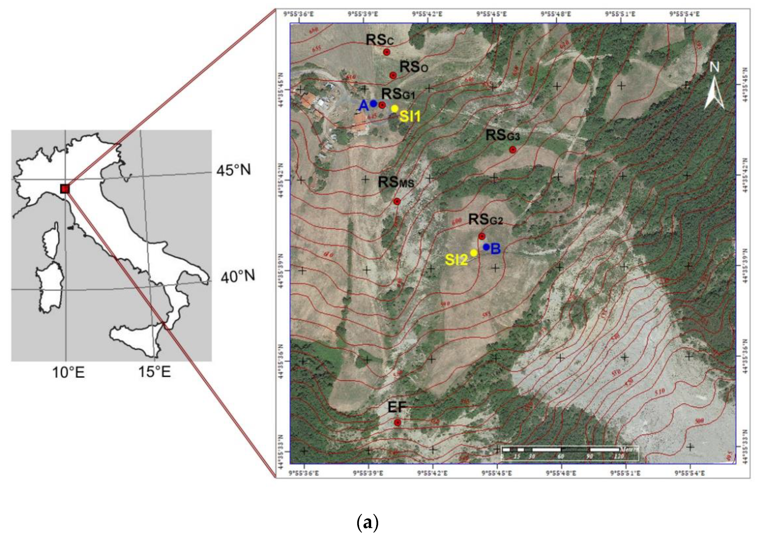
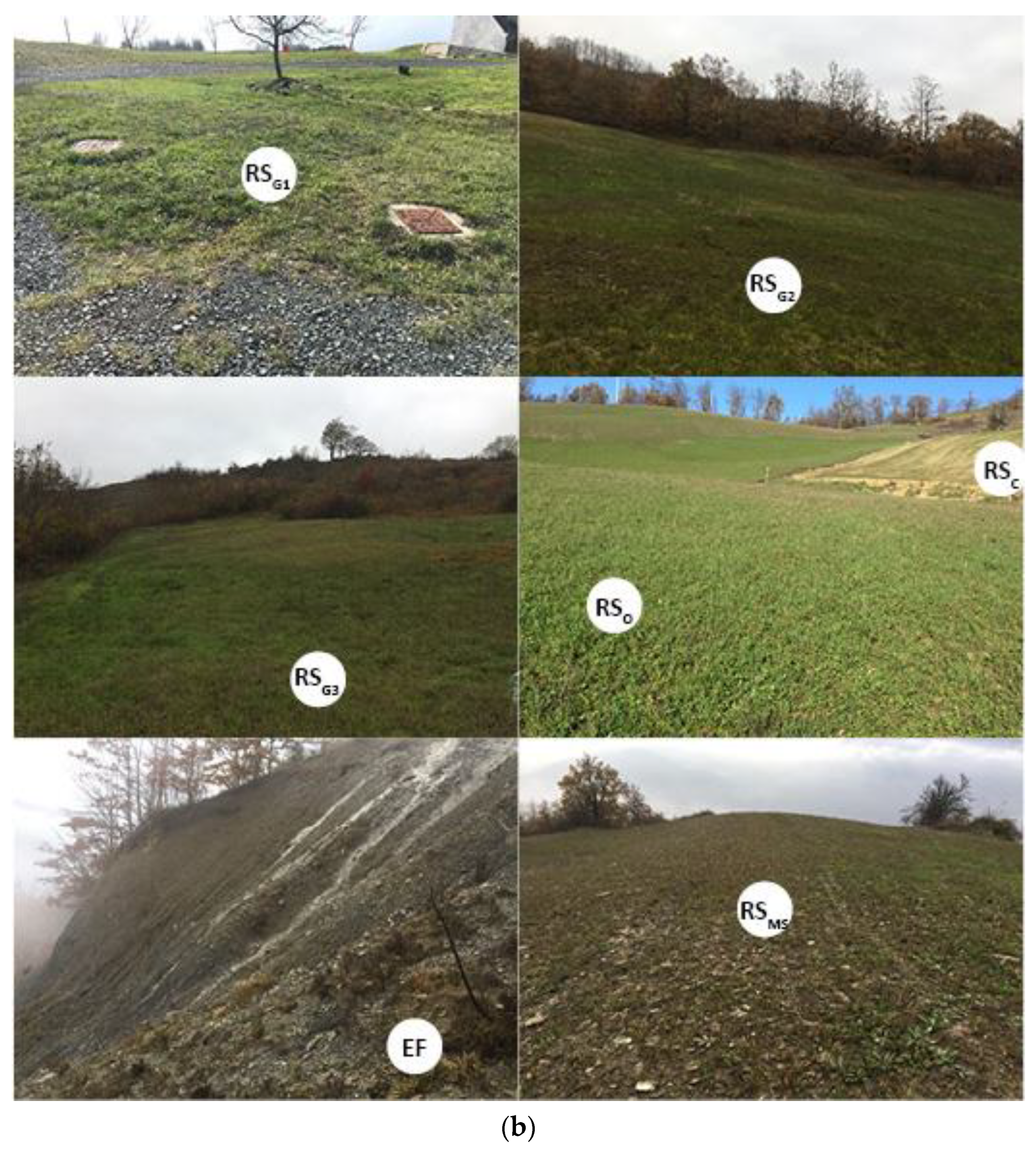
2.1. Study Area

The study area (Case Pennetta landslide) is located in the Taro River valley (Northern Apennines). During the past 25 years, the local climate condition has been characterized by annual mean precipitation ranging from 938 to 1230 mm, and annual mean temperature between 11.0–12.4 °C [10].

In the area, three tectonic units belonging to the Ligurian Domain of the Northern Apennines [21] outcrop. In detail, the geological sequence can be described as follows (from the top to the bottom of the slope): (i) Arenarie di Scabiazza (SCB), made up of thin layers of claystone alternating with sandstone layers, 15 to 20 cm thick, that gradually change from thin to very thin sandstone layers ending with marls; (ii) Argille a Palombini di Monte Rizzone (AMR), made up of claystones and intercalated decimetric limestone beds. Locally, AMR disappears and SCB lies directly on the rocks of the underlying Ottone tectonic unit, which is made of claystones containing clasts and blocks of limestone (Argille a blocchi, CCVb); (iii) these lie directly (tectonic boundary) on the underlying Flysch of Monte Caio (CAO), which is made up of thick beds of marly-limestones turbidites and intercalated thin-to-medium argillite beds. All the rocks are deeply tectonised and the layering is locally completely destroyed.

Steep surfaces and scarps usually characterize the lower portion of the studied slope, where the thick beds of marly-limestones turbidites (CAO) crop out. Conversely, milder and smooth landforms are usually found in the upper portion, due to prevailing rocks containing clay and claystone (AMR, CCVb), with the exclusion of the areas affected by landslides.

The main known reactivations of the Case Pennetta landslide occurred in 1916, 1927 and 2000–2001. During this last event, a state road and the Parma-La Spezia railway were involved in the mass movement. Moreover, new surficial effects of the slope’s instability have been detected since 2010, both in the fields (cracks and changes in slope shape and dip), and on structures and houses (tilting and microcracks). The landslide’s rate of movement was usually in the order of a few mm/year to a few cm/year (from extremely slow to very slow in the velocity scale by Cruden and Varnes [22]), even though some acceleration was observed during total reactivation events (e.g., in 1927 and in 2001). In the past, the landslide underwent a limited number of interventions, essentially in underground and surficial drainage systems.

2.2. Geological and Geomorphological Survey

The landforms were mapped by merging geomorphological maps and different datasets [23]. A digital surface model (DSM) of the study site was constructed via photogrammetric mapping using an unmanned aerial vehicle (UAV). DSM was later converted onto a digital terrain model (DTM) voiding vegetation with terrain contours from available digital cartography. Differential GPS measurements provided ground control points for UAV images and also benchmarks for areas covered by vegetation. Elevation contour lines, available from Regional Technical Cartography at scale 1:5000 [23] were utilized to fill in data gaps. The different data types were finally interpolated on a 1 m aperture mesh using a kriging algorithm.

Investigations were performed to acquire the subsurface geological features. Two corings (SI1 and SI2) were drilled within the study site at different depths beneath the field surface (Figure 1a).

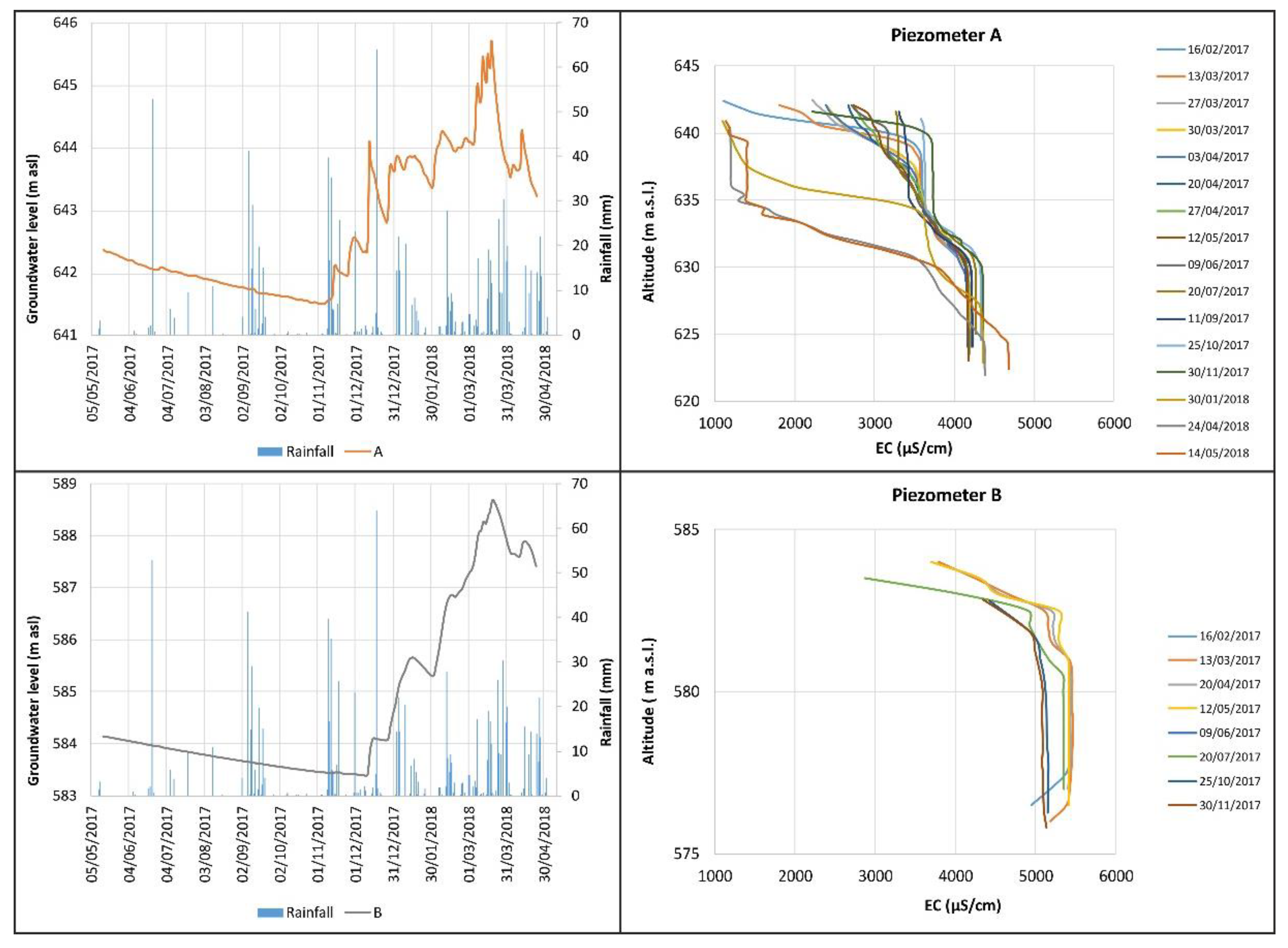
2.3. Hydrogeological Investigations

Two piezometers were drilled to measure the hydraulic head fluctuations and the groundwater electrical conductivity (EC) profiles within the investigated groundwater (Figure 1a). Piezometer A is 25-m deep and screened between 1 and 25 m below ground (623 to 648 m a.s.l.). Piezometer B is 15m deep and screened between 3 and 15 m below ground (576 to 588 m a.s.l.). Both piezometers were drilled very close to the cores SI1 and SI2 (Figure 1a).

In each of the two piezometers, a pressure transducer with data-logger (STS DL.OCS/N/RS485) was installed to monitor the hydraulic head on an hourly basis, from May 2017 to May 2018. The same piezometers were used to measure the hydraulic head through a water level meter, on a monthly basis from April 2017 onwards.

The EC of groundwater was measured inside the screened interval of each piezometer, in order to analyse possible haloclines and use the groundwater EC to investigate the hydrogeological behaviour of the studied system, according to previous studies [24,25,26,27]. EC vertical profiles were measured on a monthly basis with a borehole probe (SOLINST TLC), from April 2017 to May 2018. Measurements were carried out at 1-m-depth intervals. The effectiveness of EC values was always verified through laboratory analyses.

2.4. Soil Samples and Chemical Analysis

Soil samples were collected in seven sites located in the study area: six of those were taken from the area affected by the rotational slide and one from the earth flow (

Table 1. Sampling sites characteristics.

Site Code	Movement Type	Land Use	Coordinates (UTM)
EF	Earth flow	Eroded zone belonging to the active earth flow area	32N 573645 4938131
RSC	Rotational slide	Wheat cultivated field	32N 573634 4938510
RSG1	Rotational slide	Permanent grassland	32N 573628 4938442
RSG2	Rotational slide	Permanent grassland	32N 573732 4938321
RSG3	Rotational slide	Permanent grassland	32N 573764 4938410
RSMS	Rotational slide	Main scarp with scarce vegetation cover	32N 573645 4938357
RSO	Rotational slide	Overgrown field	32N 573641 4938486

; Figure 1a,b). The sites were selected within the rotational slide to analyse differences (i) among the land use types (cultivated, overgrown, grassland) observed at the study area, and (ii) between the main scarp and the flat areas.

Soil samples were collected for chemical analysis according to FAO recommendations [28]. Nine soil subsamples were used to perform pH and soil organic matter (SOM) analyses. pH analysis was conducted by placing a pH meter in a soil:distilled water liquid mixture in ratio 1:2.5 [29]; SOM was determined by using LOI-Loss on Ignition according to Ball’s method [30], and igniting 1 g of dried soil at 450 °C for 4 h.

2.5. Soil Arthropod Investigation

Three soil samples (10 × 10 × 10 cm³) were collected from each site in November 2018 for soil microarthropod extraction. Arthropod extraction was performed via the Berlese–Tüllgren funnel (2 mm sieve mesh; extraction time 10 days), and the specimens were placed in a preservative solution (75% ethyl alcohol and 25% glycerol by volume). Class taxonomic level for Myriapoda, and order level for Hexapoda, Chelicerata and Crustacea [31] were considered. Collembola and Acari are generally the two most present groups, in terms of species diversity and abundance, so these two groups were studied more in-depth. Collembola were classified at family level, and Acari were divided between Oribatida and other Acari. The number of specimens present for each group was counted and their abundance (ind/m²) registered. Number of taxa (NT) and Acari-to-Collembola ratio (A/C) [32] were calculated on the basis of this classification level.

2.6. Statistical Analysis

The Pearson correlation coefficient was used to determine if there was a relation between pH and SOM. The Kruskal–Wallis test for multiple comparison was performed to establish if the study sites differed in pH and SOM. Where significance was found (p ≤ 0.05), pairwise multiple comparisons between sites according to Conover were made as post-hoc.

Total abundance, number of taxa as well as abundance of taxa always present in the study sites and Acari/Collembola ratio were compared by using the Conover test as done for environmental parameters. The Akaike’s Information Criterion (AIC) was used to establish the best model to study soil fauna community data matrix. The R package “vegan” was used for arthropod communities to observe variance in community composition depending on the study site and its environmental characteristics. The Bray–Curtis distance was calculated as a measure of the dissimilarity between sites in the composition of the edaphic community, considering both the presence and the abundance of the different groups found; true abundances were log-transformed according to Borcard [33], in order to avoid placing the same importance on absolute differences in abundance without considering their order of magnitude. The same tests performed to study total community composition were conducted for Collembola communities. All data were analysed using R version 3.5.2 (R Core Team, Vienna, Austria) [34].

3. Results

3.1. Geological and Geomorphological Features of the Landslide

The Case Pennetta landslide extends from 650 m a.s.l. to the Taro riverbed (265 m a.s.l.). Its length is about 1600 m, and its maximum width is approximately 130 m. The geomorphological map (Figure 2) shows the landslide’s main landforms, with emphasis on the portions analysed within this study (rotational slide and upper part of the earth flow). The well-developed main scarp, characterised by a concave longitudinal topographic profile, and the head surface (in the counter-slope) account for a typical rotational movement.

This kinematic type pertains to the depleted mass of the landslide that extends down to 510 m a.s.l., where the toe of the failure surface is masked by the materials accumulated. Earth flows start from the front of this depleted mass and reach the Taro River, representing the foot of the landslide.

The rotational part of the landslide affects SCB and marginally AMR. Core SI1 (Figure 1a) shows, down to 30–31 m below ground (b.g.; 616–615 m a.s.l.), a matrix supported deposit characterized by a clay-silty matrix, clasts of different size (0.5 to 12 cm). From 31 m to 34 m b.g. the deposit is clast-supported and poorer in matrix compared to the upper portion. The top of the bedrock was detected at 35 m b.g. (612 m a.s.l.). Between 6–9 m and 11–14 m b.g., there is an alternation of compact and loose levels with a certain degree of disaggregation. Between 21 m and 23 m b.g., the rocks are more disaggregated. Core SI2 (Figure 1a) shows clasts and blocks of different size (from grains to 12 cm) with abundant silty-clay matrix, from the ground surface to 20 m b.g. A level richer in clay was observed at 14–15 m b.g. Dispersed organic material has also been found in the first 20 m of coring. Between 20 and 23 m b.g., the deposit is clast-supported, with clasts up to 10 cm in size. Between 21 and 21.50 m b.g. the matrix is more abundant than in the other portion of this depth interval. At 23 m b.g. (561 m a.s.l.), the rock is made of thin layers of claystone and sandstones (SCB).

3.2. Hydrogeological Behaviour

Hydraulic head measurements show several peaks during infiltration events (Figure 3), therefore suggesting rapid percolation of water from the ground surface towards the saturated zone. The groundwater EC varies significantly with depth, and the haloclines show variations over time, strictly related to local precipitations (see examples in Figure 3). Therefore, according to the results obtained in other sites [26,35], these EC variations depend on the effective infiltration of local rainwater that determines the mixing between lower-salinity fresh infiltration waters and higher-salinity pre-event groundwater. In both piezometers A and B, the EC in groundwater varies significantly with depth (Figure 3), with a great difference between the bottom (e.g., >4000 μS/cm in piezometer A) and the top value (e.g., around 1000 μS/cm in piezometer A). A step-like shape is observed in both wells. In each of the wells, the EC steps were always detected at the same depth.

On the whole, the hydrogeological investigations depict (i) a near-surface medium that is characterised by both porosity and permeability higher than those expected in clay-rich sediments (see rapid effective infiltration and arrival of fresh-infiltration waters at the groundwater table), and (ii) relatively low salinity of waters percolating through the unsaturated zone.

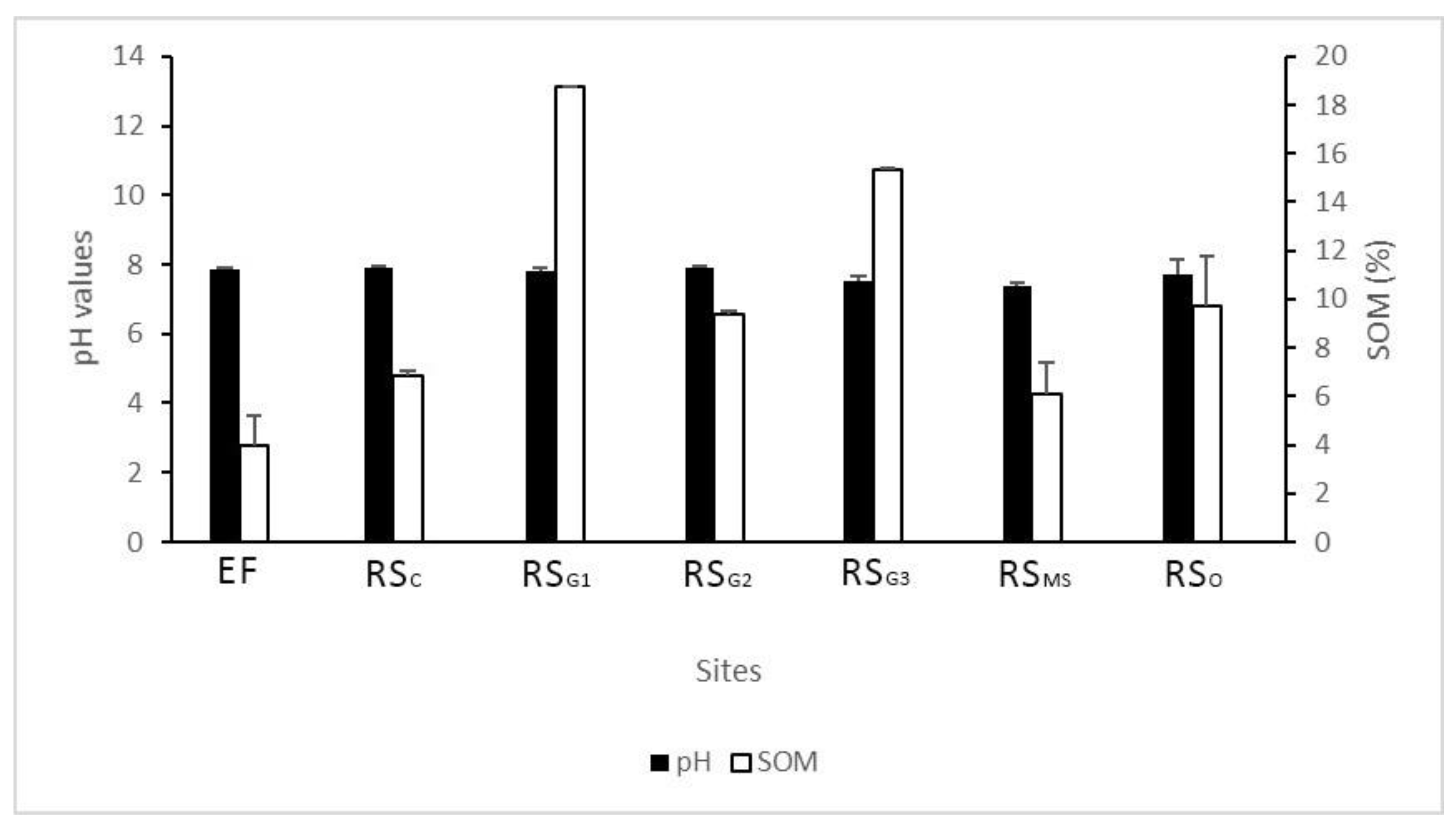
3.3. Soil Characterization

Results of pH and SOM are shown in Figure 4. The different pH values, from neutral to moderately alkaline, were not significantly distinct from each other, while percentages of SOM depended on the sampling sites (p < 0.05). In the RS_G1, SOM appeared to be higher than in the RS_C, RS_MS (p < 0.05) and EF areas (p < 0.01), in which it was significantly lower than in RS_G2 and RS_G3 (p ≤ 0.05; p < 0.01). According to the Pearson correlation, there was no relation between SOM and pH found in this study area.

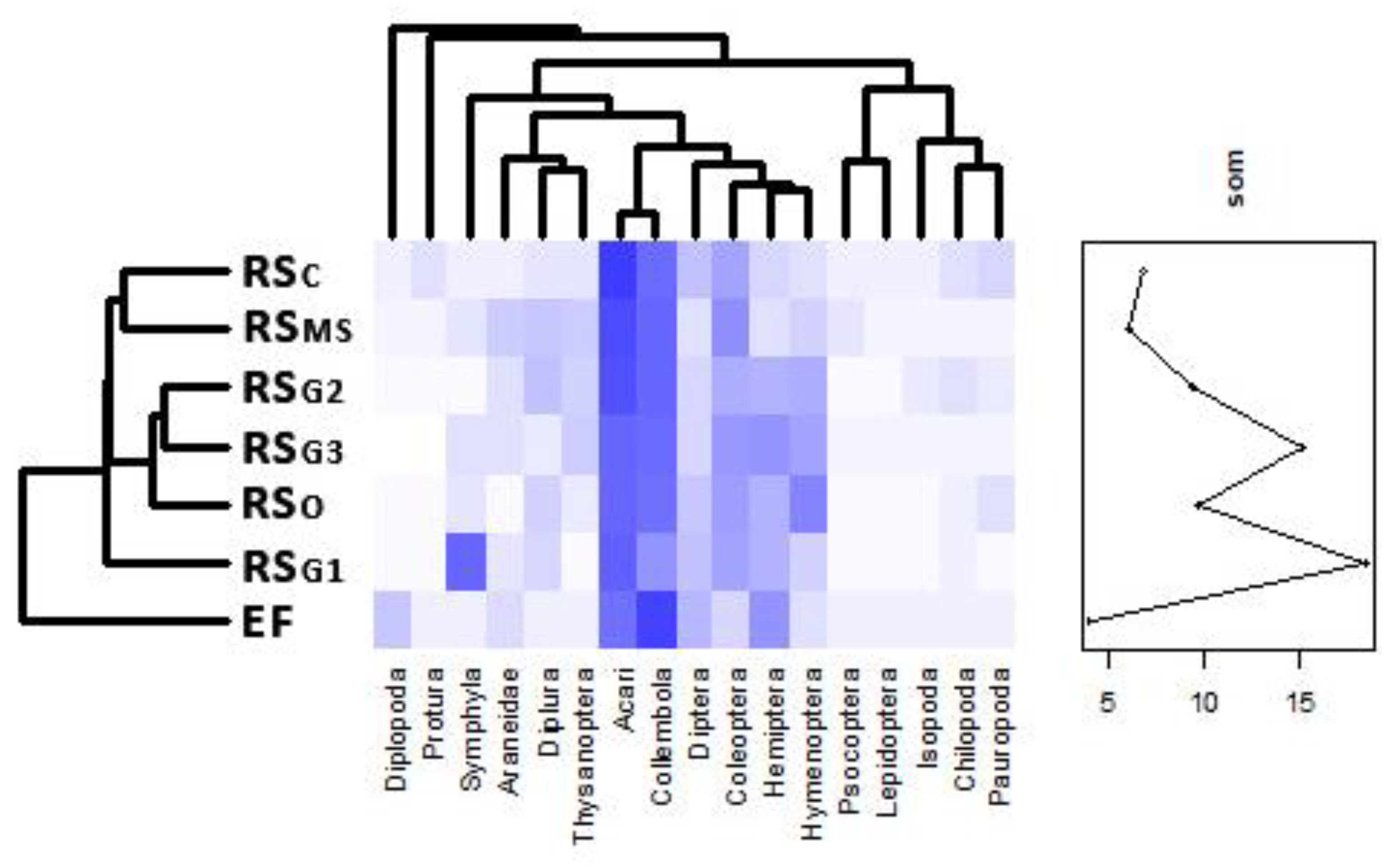
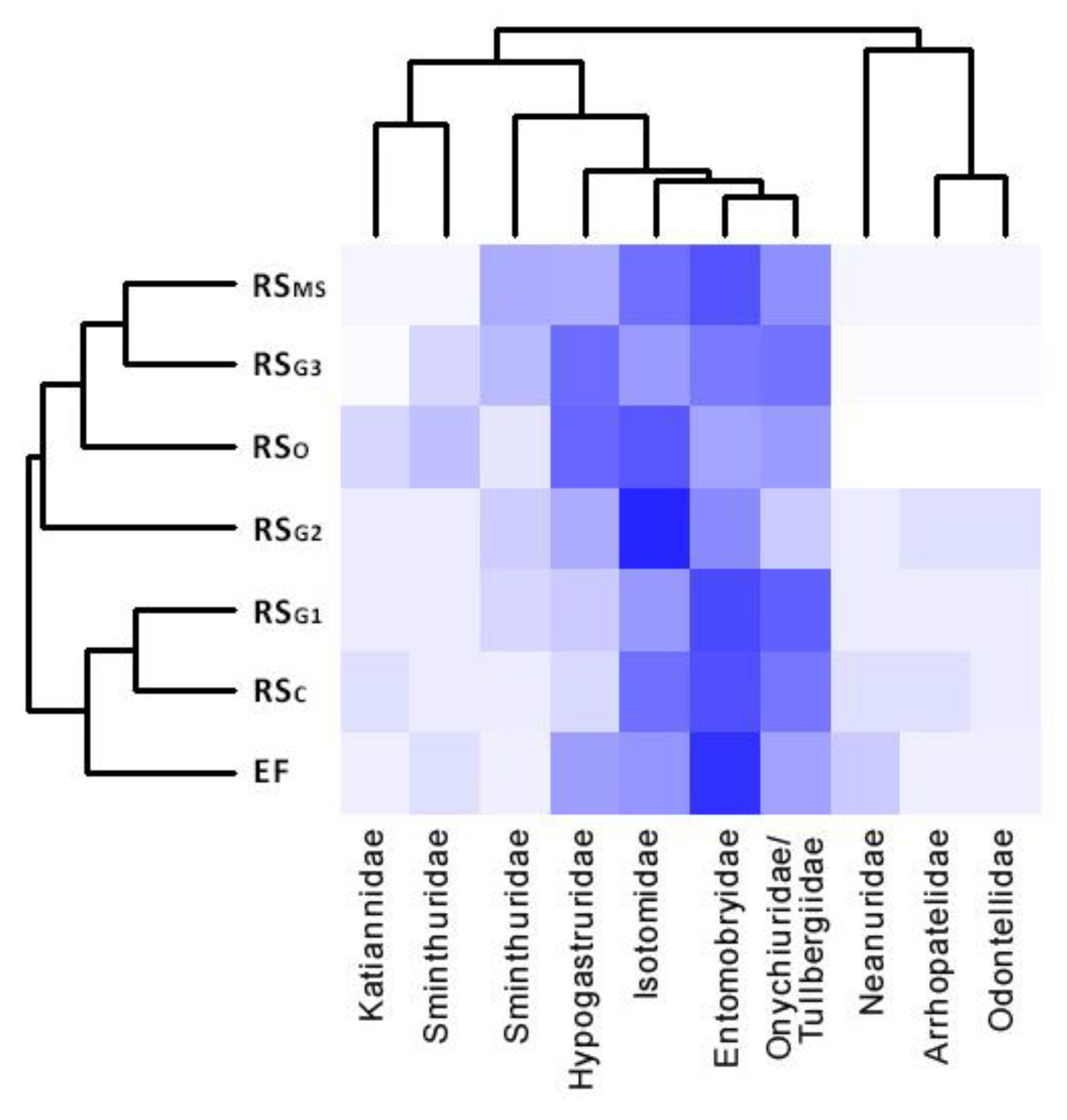
3.4. Soil Microarthropod Community

Table 2. Average ± standard error of the number of individuals (ind./m²) for each faunal group, the number of groups, the total abundance (ind./m²) and the ratio Acari/Collembola found in the seven sites studied.

Faunal Group	EF	RSc	RSG1	RSG2	RSG3	RSMS	RSO
Acari	311 ± 79	7268 ± 5867	7844 ± 447	27,588 ± 2654	4681 ± 313	6008 ± 3273	4897 ± 1345
Araneidae	14 ± 7		21 ± 0	42 ± 12	42 ± 12	64 ± 37	-
Chilopoda	-	14 ± 7	11 ± 6	42 ± 25	11 ± 6	-	7 ± 7
Coleoptera	14 ± 7	255 ± 131	573 ± 123	499 ± 67	796 ± 190	594 ± 294	566 ± 209
Larvae	-	255 ± 161	541 ± 244	403 ± 74	786 ± 196	531 ± 305	559 ± 203
Collembola	870 ± 492	1755 ± 494	1040 ± 123	10,870 ± 650	3917 ± 1122	2420 ± 735	3276 ± 1769
Diplopoda	28 ± 19	-	-	-	-	-	-
Diplura	-	7 ± 7	53 ± 18	202 ± 80	21 ± 12	74 ± 18	64 ± 25
Diptera	50 ± 7	78 ± 58	159 ± 43	74 ± 18	74 ± 6	21 ± 7	120 ± 57
Larvae	14 ± 7	64 ± 44	42 ± 21	64 ± 25	11 ± 6	11 ± 7	64 ± 12
Hemiptera	142 ± 131	28 ± 14	276 ± 86	393 ± 153	902 ± 337	21 ± 12	248 ± 146
Hymenoptera	7 ± 7	-	85 ± 37	510 ± 270	510 ± 221	42 ± 25	1720 ± 1481
Isopoda	-	-	-	21 ± 12	11 ± 6	-	-
Lepidoptera	-	-	-	-	11 ± 6	-	-
Larvae	-	-	-	-	11 ± 6	-	-
Pauropoda	-	28 ± 19	-	21 ± 12	11 ± 6	-	28 ± 14
Protura	-	14 ± 14	-	-	-	-	-
Psocoptera	-	-	-	-	11 ± 6	11 ± 6	-
Symphyla	-	-	6496 ± 2415	-	42 ± 12	11 ± 6	21 ± 12
Thysanoptera	-	7 ± 7	-	117 ± 6	106 ± 61	53 ± 31	14 ± 7
Number of groups	8 ± 1	10 ± 0	10 ± 0	11 ± 1	13 ± 1	10 ± 1	10 ± 0
Total abundance	1437 ± 709	9469 ± 5699	16,559 ± 2674	40,379 ± 3711	11,146 ± 1243	9320 ± 4380	10,962 ± 3910
Acari/Collembola	2 ± 1	6 ± 5	8 ± 1	3 ± 0	1 ± 0	2 ± 1	2 ± 1

shows the results of soil microarthropod community. Overall, 17 taxa were found in the study area, five of which found in all sites: Acari, Coleoptera, Collembola, Diptera and Hemiptera. The greatest total abundance per m² was found in RS_G2, statistically higher than RS_C, RS_MS, RS_G3 (p ≤ 0.05) and EF (p < 0.01); EF showed the lowest abundance, less than in RS_O and RS_G1 (p < 0.05). RS_C and EF areas revealed a significantly lower number of groups than the other sites (p ≤ 0.05), except for the comparison between RS_C and RS_G1, and between both RS_C and EF, and RS_MS. The best model to study soil fauna community data matrix was considering site and SOM as independent variables, with the result that each one contributed significantly to edaphic community composition (p < 0.01 and p ≤ 0.05 respectively). The Bray–Curtis distance denoted the greatest dissimilarity (from 38% to 50%) between EF and the other sites, particularly RS_G2, while fauna composition appeared to be similar for over 80% between RS_G2, RS_G3 and RS_O (Figure 5).

Greater Acari abundance was found in RS_G2, significantly higher than in RS_C (p < 0.05) and EF sites (p < 0.01); in EF their presence was lower than RS_O and RS_G1 (p < 0.05). Among them, a distinction was made between those belonging to Oribatida and to other Acari (Figure 6). The Acari community strongly depends on the site (p ≤ 0.01); with EF abundance of Oribatida significantly lower than that of the other sites (p < 0.05) except for RS_C (lower than RS_G2, p < 0.05) and RS_MS. The abundance of Oribatida was greater than other Acari in RS_G3 and RS_O only.

Like Acari, less abundant Coleoptera and Collembola were found in EF. The number of Coleoptera in EF was lower than in RS_G3 and in RS_O (p < 0.05). The abundance of Collembola observed in RS_G2 was statistically greater than in RS_G1 and in EF (p < 0.05, p < 0.01). Ten Collembola families were identified (

Table 3. Average ± standard error of the number of Collembola per m².

Collembola Family	EF	RSC	RSG1	RSG2	RSG3	RSMS	RSO
Arrhopalitidae	-	7 ± 7	-	11 ± 6	-	-	-
Entomobryidae	623 ± 429	934 ± 532	563 ± 67	393 ± 80	955 ± 110	1306 ± 215	205 ± 51
Hypogastruridae	71 ± 51	14 ± 7	21 ± 12	138 ± 18	1337 ± 735	106 ± 61	1076 ± 416
Isotomidae	85 ± 65	425 ± 170	96 ± 31	10,243 ± 766	329 ± 116	616 ± 282	1592 ± 1392
Neanuridae	21 ± 12	7 ± 7	-	-	-	-	-
Onychiuridae/Tullbergiidae	64 ± 64	361 ± 165	350 ± 67	42 ± 12	1136 ± 313	265 ± 104	255 ± 44
Odontellidae	-	-	-	11 ± 6	-	-	-
Katiannidae	-	7 ± 7	-	-	-	-	42 ± 21
Sminthuridae	-	-	11 ± 6	32 ± 6	117 ± 55	127 ± 74	21 ± 12
Sminthurididae	7 ± 7	-	-	-	42 ± 25	-	85 ± 56

), with four present in all sites: Entomobryidae, Hypogastruridae, Isotomidae and Onychiuridae/Tullbergiidae.

The whole Collembola community composition depended on the site (p < 0.01), with EF and RS_O showing the highest dissimilarity, RS_G1 and RS_C resulting more similar to each other than the other sites, and Entomobryidae and Onychiuridae/Tullbergiidae as families that occurred together more often (Figure 7). Through multiple comparison between the families always present RS_O proved to be the site with significantly fewer Entomobryidae than RS_MS and RS_G3 (p < 0.01; p < 0.05), and more Hypogastruridae than RS_C, RS_G1 and EF (p < 0.01, p < 0.01, and p < 0.05 respectively). The Hypogastruridae found in RS_C were lower than those in RS_G3, too (p < 0.05). Most Isotomidae were in RS_G2, more than in RS_C and EF (p < 0.01). The greater presence of Onychiuridae/Tullbergiidae was in RS_G3, more than RS_G2 and EF (p < 0.01), whose number was lower than in RS_C and RS_G1, too (p < 0.05).

The lowest abundance of Diptera was in the RS_MS, significantly different from RS_G1 and RS_O (p < 0.05). The only other group found in all sites was Hemiptera, which showed a higher number in RS_G3 than in RS_C, EF and RS_MS (p < 0.05). Acari/Collembola ratio, being higher in RS_G1, did not differ significantly between sites.

4. Discussion

In this research, the hydrodynamic characterization of a complex landslide was carried out to evaluate the effects of this system type on soil biodiversity, in terms of soil arthropod community, with the aim to highlight if soil fauna can be a useful tool in landslide studies.

No difference was found in soil pH, similarly to other results obtained from landslide areas by Wilcke [36]. Instead, organic matter content (SOM) varied significantly between sites. As known, soil pH and SOM alteration can highlight a soil disturbance condition and contribute to altering ecosystem biodiversity.

Not only does SOM influence nutrient availability, it also promotes soil aggregation and improves water infiltration, and its content is known to decline from grassland to cultivated areas [37].

In this study, the lowest amount of SOM was detected in the earth flow area (EF), followed by the main scarp of the rotational slide (RS_MS), and both sites were similar to the cultivated site within the rotational slide (RS_C). The differences observed between earth flow (EF) and grasslands (RS_G1, RS_G2, RS_G3) show the surface heterogeneity created after slope failure.

It is known that the slip face at the upper edge of a landslide is more unstable, subject to erosion and not readily colonized [38]. Moreover, as suggested by some authors [36], fertility reduction caused by landslides, can involve the whole area. Usually, SOM content is an important feature in driving soil faunal community, and to confirm this, our study shows an evident relationship between SOM content and soil microarthropods. On the other hand, since arthropod faeces are involved in humus production and soil aggregation, soil arthropod abundance and diversity contribute to incrementing soil structure and, consequently, soil stability. In this study, earth flow (EF) showed the poorest soil faunal community, in terms of both number of groups and abundance. Moreover, as for SOM content, soil arthropod abundance in the earth flow (EF) proved to be similar to the main scarp of the rotational slide (RS_MS) and cultivated area sampled within the rotational slide (RS_C). This result confirms that the whole landslide area (EF + RS) is involved in a soil degradation process. Indeed, the soil arthropod abundance detected in RS_G1, being similar to RS_C and lower than a typical grassland condition [39], suggests that a stressful action is affecting the area dramatically. The Collembola community supports this observation since, despite its abundance in the EF being lower than the other sites, the community structure in this site was similar to RS_G1, RS_C and RS_MS (79%, 72% and 69%, respectively). Entomobryidae was the most abundant family found in these sites and the specimens found for this family are almost all epigeic. This result suggests that these specimens were less affected by belowground disturbance as reported in previous studies [40,41]. As known, Collembola have a leading role in the soil structure making; indeed, their faeces contribute to the water-holding capacity and soil aggregation [42]. In this study, the greatest abundance of this group was found in RS_G2, whose community structure was richer than the other sites, overall for the greatest presence of Isotomidae. RS_G3 showed a high number of Onychiuridae/Tullbergiidae. As reported by Rusek [43], Onychiuridae, rare in clay soils, are known for their ability to make “microtunnels” in the soil matrix, ability shared with Oribatida Acari, thus increasing aeration and drainage.

As for the Collembola, even for Acari the abundance of this taxon was very low in EF, confirming the degradation condition of this site. Moreover, no difference was detected between Oribatida and others Acari in terms of abundance in this site. On the other hand, RS_G3, showing the greatest abundance of Oribatida, confirms the importance of a grass cover in soil biodiversity maintenance. Indeed, Oribatida are typical of stable and humid soils, rich in organic matter, since they can survive in submerged condition even over long periods of time, while they are susceptible to drought and their densities decline in man-modified areas subjected to agricultural treatments [44,45,46]. Centipedes (Chilopoda), which have a thinner cuticle and are sensitive to water stresses [47], were also found in all sites except EF, confirming the degradation condition of this site.

Contributing to SOM contents and consequently to soil resistance to erosion, organisms involved in litter breakdown can play a key role in soil structure maintenance. Coleoptera and Diptera larvae, Symphyla, Diplopoda, Isopoda and Thysanoptera were observed among the main arthropod groups found in this study that take part in this process. Abundance of Coleoptera such as Oribatida was greater in RS_O and in RS_G3 than in the other sites; both groups can affect soil structure while moving into the pores and pushing particles aside, contributing to soil porosity. Coleoptera larvae, rarely observed in EF, are good indicators of soil water content, as their permeable cuticle makes them susceptible to desiccation [48].

Considering that ants build complicated burrows deep into the ground, forming a network of macropores [49], the greater abundance of this group in RS_G2, RS_G3, and RS_O when compared to the four other sites, suggests a greater infiltration capacity of these soils. Differently from ants, abundance of Diptera was greater in RS_G1. Their presence could be related to the occasional presence of goats, factor that produces a high manure content, increasing the abundance of soil dwelling Diptera [50]. This idea is supported by the high number of Symphyla present in this site, whose abundance strongly depends on SOM content [51]. Moreover, Symphyla can give information about soil structure, since they cannot dig tunnels actively in soil and they use existing pores to move in the soil.

Isopoda is a group susceptible to water loss by evapotranspiration and live in moist habitats where they feed mainly on dead and decaying plant material. These considerations highlight that these properties are typical of RS_G2 and RS_G3, where this group was observed. Thysanoptera showed similar behaviour, having the greatest abundance in the two sites.

These results point out that soil arthropod community can influence and/or can be influenced by the hydraulic features of a low-permeability system in a landslide area. Firstly, arthropods such as Onychiuridae, Oribatida, Coleoptera, and ants are able to increase both the effective porosity and the permeability of the upper “aquifer” medium, therefore enhancing the effective infiltration of rainwater in a porous low-permeability system. Since these arthropods can increase porosity and permeability in several tens of centimetres below ground, their ability to create macropore (mm in dimension) networks causes the vertical permeability to decrease significantly with depth. Due to this vertical heterogeneity, further emphasised by plausible rock weathering, a significant contrast in permeability is expected within the shallow aquifer medium, and temporary perched groundwater could be found within the landslide area during the main rainwater events. Taking into consideration the heterogeneous distributions of the arthropods mentioned above, as well as the geological heterogeneity of the medium studied, temporary perched groundwater could be also discontinuous within the study site. This hypothesis is in agreement with the existence of several temporary springs observed at different altitudes during wintertime (data not shown).

In a wider context, the higher permeability of the shallow “aquifer” system enhances the rapid recharge of the groundwater intercepted and monitored through piezometers A and B, in agreement with the “nervous” hydraulic head fluctuation observed by means of the pressure transducers. The slight difference in time lag between rain event and hydraulic head rise observed between piezometers A and B is also in agreement with the system’s heterogeneity.

As for the bioindicator role of some arthropods, Isopoda seem to be a good indicator to detect the areas where the groundwater head comes frequently close to the ground (see examples at RS_G2 and RS_G3), due to their ability to live in moist habitat. They were actually identified in RS_G2 and RS_G3 only, where the groundwater often flows out diffusely, during the main rainwater events. On the whole, these results further emphasize the effectiveness of coupled hydrogeological–biological approaches [52].

5. Conclusions

The study suggests that the earth flow, differing from the other sites analysed within the rotational slide for its lower arthropod biodiversity and abundance, appears to be the most stressed area, exposed to erosion, and susceptible to extreme conditions, such as drought. The cultivated area sampled within the rotational slide fits with the many conventional agricultural systems, as reported in other studies, showing low arthropod biodiversity and abundance. The overgrown site instead showed a community composition more similar to RS_G3, and only partially different from RS_G2, mainly in total abundance, determined above all by Acari and Collembola densities. These three sites are characterized by good conditions in terms of grass presence and consequently rhizosphere, SOM content, water retention and porosity—all of which are important factors in supporting a complex and structured soil arthropod community. RS_G1 appears to have an intermediate situation, showing great arthropod abundance, mainly due to the high arthropod density strongly related to high SOM contents, yet, on the other hand, showing characteristics observed in disturbed and degraded soils, as the Collembola community suggested, being very similar to those observed in stressed sites.

From the methodological point of view, this study suggests the possibility to effectively merge soil fauna and hydrogeological investigations to better understand the hydraulic features and behaviour of low-permeability systems. At the same time, the approach applied is efficient to distinguish degraded soils, often associated with types of landslides, such as earth flows, that cause partial or complete soil removal, from more preserved soils. The latter are often associated with types of landslide, such as rotational or translational slides, that are characterized by movement in depth, along the sliding surface, while the upper portion of the depleted mass can remain untouched.

The use of the soil fauna as indicator of the health state of the soil in landslide areas may contribute to the evaluation of the potentiality of these surfaces for agricultural purposes. For instance, plants (like maize) or trees (like apple orchards) that need a consistent rate of water would represent kind of cultivation that could be irrigated by extracting the waters from the landslides themselves once the paths of these have been identified within the body of the landslide.

The surfaces of landslides, which are obviously not active or characterized by very slow rate of movement like in the case studied, may represent for some portions within mountain chains, such as the Italian Apennines, the only areas suitable for cultivation. In the Apennines, this fact occurred in the past when many large landslides were exploited with these purposes, and for settlements, but even today they could represent the way to restoration and re-use of these surfaces, contributing to the maintenance and care of the territory and the prevention of landslide movement.

References

1. Boccaletti, M.; Elter, P.; Guazzone, G. Plate Tectonic Models for the Development of the Western Alps and Northern Apennines. Nat. Phys. Sci. 1971, 234, 108–111. [Google Scholar] [CrossRef]
2. Kligfield, R. The northern Apennines as a collisional orogen. Am. J. Sci. 1979, 279, 676–691. [Google Scholar] [CrossRef]
3. Vai, G.B.; Martini, P. Anatomy of an Orogen: The Apennines and Adjacent Mediterranean Basins; Kluwer Academic Publishers: Tranbjerg, Denmark, 2001; ISBN 9780412750403. [Google Scholar]
4. Molli, G. Northern Apennine–Corsica orogenic system: An updated overview. Geol. Soc. Lond. Spec. Publ. 2008, 298, 413–442. [Google Scholar] [CrossRef]
5. Crozier, M.J. Landslide geomorphology: An argument for recognition, with examples from New Zealand. Geomorphology 2010, 120, 3–15. [Google Scholar] [CrossRef]
6. Carlini, M.; Chelli, A.; Vescovi, P.; Artoni, A.; Clemenzi, L.; Tellini, C.; Torelli, L. Tectonic control on the development and distribution of large landslides in the Northern Apennines (Italy). Geomorphology 2016, 253, 425–437. [Google Scholar] [CrossRef]
7. Perrone, A.; Iannuzzi, A.; Lapenna, V.; Lorenzo, P.; Piscitelli, S.; Rizzo, E.; Sdao, F. High resolution electrical imaging of the Varco d’Izzo earthflow (southern Italy). J. Appl. Geophys. 2004, 56, 17–29. [Google Scholar] [CrossRef]
8. Bertolini, G.; Corsini, A.; Tellini, C. Fingerprints of Large-Scale Landslides in the Landscape of the Emilia Apennines. In Landscapes and Landforms of Italy; Soldati, M., Marchetti, M., Eds.; Springer International Publishing: Berlin, Germany, 2017; pp. 215–224. [Google Scholar] [CrossRef]
9. Carlini, M.; Chelli, A.; Francese, R.; Giacomelli, S.; Giorgi, M.; Quagliarini, A.; Carpena, A.; Tellini, C. Landslides types controlled by tectonics-induced evolution of valley slopes (Northern Apennines, Italy). Landslides 2018, 15, 283–296. [Google Scholar] [CrossRef]
10. Antolini, G.; Pavan, V.; Tomozeiu, R.M.V. Atlante Climatico dell’Emilia-Romagna 1961–2015; ARPAe: Bologna, Italy, 2017; ISBN 9788887854442. [Google Scholar]
11. Jongman, B.; Hochrainer-Stigler, S.; Feyen, L.; Aerts, J.C.J.H.; Mechler, R.; Botzen, W.J.W.; Bouwer, L.M.; Pflug, G.; Rojas, R.; Ward, P.J. Increasing stress on disaster-risk finance due to large floods. Nat. Clim. Chang. 2014, 4, 264–268. [Google Scholar] [CrossRef]
12. Palis, E.; Lebourg, T.; Vidal, M.; Levy, C.; Tric, E.; Hernandez, M. Multiyear time-lapse ERT to study short- and long-term landslide hydrological dynamics. Landslides 2017, 14, 1333–1343. [Google Scholar] [CrossRef]
13. Bièvre, G.; Jongmans, D.; Goutaland, D.; Pathier, E.; Zumbo, V. Geophysical characterization of the lithological control on the kinematic pattern in a large clayey landslide (Avignonet, French Alps). Landslides 2016, 13, 423–436. [Google Scholar] [CrossRef]
14. Segoni, S.; Piciullo, L.; Gariano, S.L. A review of the recent literature on rainfall thresholds for landslide occurrence. Landslides 2018, 15, 1483–1501. [Google Scholar] [CrossRef]
15. Lissak, C.; Maquaire, O.; Malet, J.P.; Bitri, A.; Samyn, K.; Grandjean, G.; Bourdeau, C.; Reiffsteck, P.; Davidson, R. Airborne and ground-based data sources for characterizing the morphostructure of a coastal landslide. Geomorphology 2014, 217, 140–151. [Google Scholar] [CrossRef]
16. Geertsema, M.; Pojar, J.J. Influence of landslides on biophysical diversity—A perspective from British Columbia. Geomorphology 2007, 89, 55–69. [Google Scholar] [CrossRef]
17. Geertsema, M.; Highland, L.; Vaugeouis, L. Environmental Impact of Landslides. In Landslides—Disaster Risk Reduction; Springer: Berlin/Heidelberg, Germany, 2009; pp. 589–607. ISBN 9783540699705. [Google Scholar] [CrossRef]
18. Pimentel, D. Soil erosion: A food and environmental threat. Environ. Dev. Sustain. 2006, 8, 119–137. [Google Scholar] [CrossRef]
19. Wardle, D.A.; Bardgett, R.D.; Klironomos, J.N.; Setälä, H.; van der Putten, W.H.; Wall, D.H. Ecological linkages between aboveground and belowground biota. Science 2004, 304, 1629–1633. [Google Scholar] [CrossRef]
20. Smith, R.B.; Commandeur, P.R.; Ryan, M.W. Soils, Vegetation, and Forest Growth on Landslides and Surrounding Logged and Old-Growth Areas on the Queen Charlotte Islands; BC Land Management Report; Ministry of Forests: Victoria, BC, Canada, 1986; Volume 41, p. 95.
21. Vescovi, P. Note Illustrative Della Carta Geologica D’italia Alla Scala 1:50.000. Foglio 216 Borgo Val di Taro; Servizio Geologico d’Italia-Regione Emilia Romagna: Roma, Italy, 2002; p. 115. [Google Scholar]
22. Cruden, D.M.; Varnes, D.J. Landslide Types and Processes, Special Report. In Landslides: Investigation and Mitigation; Turner, A.K., Shuster, R.L., Eds.; National Academy Press: Washington, DC, USA, 1996; Volume 247, pp. 36–75. [Google Scholar]
23. Cartografia Interattiva e Banche Dati. Available online: Ambiente.regione.emilia-romagna.it/it/geologia/cartografia/webgis-banchedati (accessed on 5 August 2019).
24. Morin, R.H.; Carleton, G.B.; Poirier, S. Fractured-aquifer hydrogeology from geophysical logs; the passaic formation, New Jersey. Ground Water 1997, 35, 328–338. [Google Scholar] [CrossRef]
25. Cook, P.G.; Love, A.J.; Dighton, J.C. Inferring ground water flow in fractured rock from dissolved radon. Ground Water 1999, 37, 606–610. [Google Scholar] [CrossRef]
26. Petrella, E.; Naclerio, G.; Falasca, A.; Bucci, A.; Capuano, P.; De Felice, V.; Celico, F. Non permanent shallow halocline in a fractured carbonate aquifer, southern Italy. J. Hydrol. 2009, 373, 267–272. [Google Scholar] [CrossRef]
27. Aquino, D.; Petrella, E.; Florio, M.; Celico, P.; Celico, F. Complex hydraulic interactions between compartmentalized carbonate aquifers and heterogeneous siliciclastic successions: A case study in southern Italy. Hydrol. Process. 2015, 29, 4252–4263. [Google Scholar] [CrossRef]
28. FAO. Guidelines for Profile Description, 3rd ed.; Soil Resources, Management and Conservation Service, Land and Water Development Division; FAO: Rome, Italy, 1990. [Google Scholar]
29. Jackson, M.L. Soil Chemical Analysis; Prentice Hall, Inc.: Englewood Cliffs, NJ, USA, 1958; 498 S. DM 39.40. Zeitschrift für Pflanzenernährung Düngung Bodenkd. 2007, 85, 251–252. [Google Scholar] [CrossRef]
30. Ball, D.F. Loss-On-Ignition As An Estimate Of Organic Matter And Organic Carbon In N -Calcareous Soils. J. Soil Sci. 1964, 15, 84–92. [Google Scholar] [CrossRef]
31. The Taxonomicon. Available online: http://taxonomicon.taxonomy.nl/ (accessed on 5 August 2019).
32. Bachelier, P.G. La vie Animale Dans les sols I. -Déterminisme de la Faune des Sols; ORSTOM: Paris, France, 1963. [Google Scholar]
33. Borcard, D.; Gillet, F.; Legendre, P.; Borcard, D.; Gillet, F.; Legendre, P. Association Measures and Matrices. In Numerical Ecology with R; Springer: New York, NY, USA, 2011; pp. 31–51. ISBN 978-1-4419-7975-9. [Google Scholar] [CrossRef]
34. R Core Team. R: A Language and Environment for Statistical Computing; R Foundation for Statistical Computing: Vienna, Austria, 2018; Available online: https://www.R-project.org/ (accessed on 23 February 2019).
35. Petrella, E.; Celico, F. Mixing of water in a carbonate aquifer, southern Italy, analysed through stable isotope investigations. Int. J. Speleol. 2013, 42, 25–33. [Google Scholar] [CrossRef] [Green Version]
36. Wilcke, W.; Valladarez, H.; Stoyan, R.; Yasin, S.; Valarezo, C.; Zech, W. Soil properties on a chronosequence of landslides in montane rain forest, Ecuador. CATENA 2003, 53, 79–95. [Google Scholar] [CrossRef]
37. Chibsa, T.; Ta, A.A. Assessment of Soil Organic Matter under Four Land Use Systems in the Major Soils of Bale Highlands, South East Ethiopia b. Factors Affecting Soil Organic Matter Distribution. World Appl. Sci. J. 2009, 6, 1506–1512. [Google Scholar]
38. Walker, L.R.; Velázquez, E.; Shiels, A.B. Applying lessons from ecological succession to the restoration of landslides. Plant Soil 2009, 324, 157–168. [Google Scholar] [CrossRef]
39. Menta, C.; Leoni, A.; Gardi, C.; Conti, F. Are grasslands important habitats for soil microarthropod conservation? Biodivers. Conserv. 2011, 20, 1073–1087. [Google Scholar] [CrossRef]
40. Parisi, V.; Menta, C.; Gardi, C.; Jacomini, C.; Mozzanica, E. Microarthropod Communities as a Tool to Assess Soil Quality and Biodiversity: A new Approach in Italy. Agric. Ecosyst. Environ. 2005, 105, 323–333. [Google Scholar] [CrossRef]
41. Parisi, V.; Menta, C. Microarthropods of the soil: Convergence phenomena and evaluation of soil quality using QBS-ar and QBS-c. Fresenius Environ. Bull. 2008, 17, 1170–1174. [Google Scholar]
42. Van Vliet, P.C.J.; Hendrix, P.F. Role of fauna in soil physical processes. In Soil Biological Fertility: A Key to Sustainable Land Use in Agriculture; Springer: Dordrecht, The Netherlands, 2007; pp. 61–80. ISBN 9781402066184. [Google Scholar] [CrossRef]
43. Rusek, J. Soil microstructures-contributions on specific soil organisms. Quest. Entomol. 1985, 21, 497–514. [Google Scholar]
44. Schatz, H.; Behan-Pelletier, V. Global diversity of oribatids (Oribatida: Acari: Arachnida). Hydrobiologia 2008, 595, 323–328. [Google Scholar] [CrossRef]
45. Maraun, M.; Scheu, S. The Structure of Oribatid Mite Communities (Acari, Oribatida): Patterns, Mechanisms and Implications for Future Research. Ecography 2000, 23, 374–383. [Google Scholar] [CrossRef]
46. Gergocs, V.; Hufnagel, L. Application of Oribatid Mites as Indicators (Review). Appl. Ecol. Environ. Res. 2009, 7, 79–98. [Google Scholar] [CrossRef]
47. Lavelle, P. (Patrick); Spain, A.V. Soil organisms. In Soil ecology; Springer Science & Business Media, Ed.; Springer: Dordrecht, The Netherlands, 2007; p. 654. ISBN 9780306481628. [Google Scholar]
48. Brown, V.K.; Gange, A.C. Insect Herbivory Insect Below Ground. Adv. Ecol. Res. 1990, 20, 1–58. [Google Scholar]
49. Gabet, E.J.; Reichman, O.J.; Seabloom, E.W. The effects of bioturbation on soil processes and sediment transport. Annu. Rev. Earth Planet. Sci. 2003, 31, 249–273. [Google Scholar] [CrossRef]
50. Frouz, J. Use of soil dwelling Diptera (Insecta, Diptera) as bioindicators: A review of ecological requirements and response to disturbance. Agric. Ecosyst. Environ. 1999, 74, 167–186. [Google Scholar] [CrossRef]
51. Edwards, C.A. The ecology of Symphyla. Entomol. Exp. Appl. 1958, 1, 308–319. [Google Scholar] [CrossRef]
52. Petrella, E.; Bucci, A.; Ogata, K.; Zanini, A.; Naclerio, G.; Chelli, A.; Francese, R.; Boschetti, T.; Pittalis, D.; Celico, F. Hydrodynamics in Evaporate-Bearing Fine-Grained Successions Investigated through an Interdisciplinary Approach: A Test Study in Southern Italy—Hydrogeological Behaviour of Heterogeneous Low-Permeability Media. Geofluids 2018, 2018. [Google Scholar] [CrossRef]
Figure 1. (a) Location of the piezometers (blue points), the corings (yellow points) and the soil sampling sites (red points) (the contour lines show the altitude in meters above sea level); (b) Sampling sites: RSG1: Rotational Slide-Grassland 1; RSG2: Rotational Slide-Grassland 2; RSG3: Rotational Slide-Grassland 3; RSO: Rotational Slide-Overgrown; RSC: and Rotational Slide-Cultivated; EF: Earth Flow; RSMS: Rotational Slide-Main Scarp.
Water 11 01882 g001aWater 11 01882 g001b
Figure 2. Geomorphological map. The contour lines show the altitude in meters above sea level.
Water 11 01882 g002
Figure 3. Hydraulic head fluctuations measured in piezometers A and B, and daily precipitation recorded at Mormorola station and the vertical profile of electrical conductivity (EC) in piezometers A and B.
Water 11 01882 g003
Figure 4. Average and standard error of the pH and SOM found in each site.
Water 11 01882 g004
Figure 5. Heat map of the community composition, with colour intensities proportional to taxa abundance, and UPGMA (unweighted pair-group method using arithmetic averages) clustering of a matrix of Bray–Curtis distance among sites (on the left side) and of the taxa that occur more often together (on the top side); on the right side, the SOM values are displayed.
Water 11 01882 g005
Figure 6. Average and standard error of the number of Oribatida and others Acari (ind./m2) found in each site.
Water 11 01882 g006
Figure 7. Heat map of the Collembola community composition, with colour intensities proportional to family abundance, and UPGMA (unweighted pair-group method using arithmetic averages) clustering of a matrix of Bray–Curtis distance among sites (on the left side) and of the families that occur more often together (on the top side).
Water 11 01882 g007