A Comprehensive Performance Assessment of the Modified Philip–Dunne Infiltrometer

Abstract

This study aims at furthering our understanding of the Modified Philip–Dunne Infiltrometer (MPDI), which is used to determine the saturated hydraulic conductivity K_s and the Green–Ampt suction head Ψ at the wetting front. We have developed a forward-modeling algorithm that can be used to simulate water level changes inside the infiltrometer with time when the soil hydraulic properties K_s and Ψ are known. The forward model was used to generate 30,000 water level datasets using randomly generated values of K_s and Ψ values. These model data were then compared against field-measured water level drawdown data collected for three types of soil. The Nash–Sutcliffe efficiency (NSE) was used to assess the quality of the fit. Results show that multiple sets of the model parameters K_s and Ψ can yield drawdown curves that can fit the field-measured data equally well. Interestingly, all the successful sets of parameters (delineated by NSE ≥ the threshold value) give K_s values converged to a valid range that is fully consistent with the tested soil texture class. However, Ψ values varied significantly and did not converge to a valid range. Based on these results, we conclude that the MPDI is a useful field method to estimate K_s values, but it is not a robust method to estimate Ψ values. Further studies are needed to improve the experimental procedures that can yield more sensitive data that can help uniquely identify K_s and Ψ values.

1. Introduction

Saturated hydraulic conductivity K_s is one of the most important parameters that control the water seepage processes through the soil profile [1,2,3,4,5]. The value of K_s depends on the size and type of mineral present in the soil; for example, the presence of fine minerals such as silt and clay can greatly reduce K_s values [6,7,8,9]. In addition, the value of K_s decreases with a reduction in the effective porosity of the system [9,10,11].

Analyzing the undisturbed soil core taken from the field is a common method to determine K_s in the laboratory using either the constant- or falling-head permeameter [12]. The soil core method has some challenges including macropores created by insertion of the ring, and relatively small sample size that may not yield a representative K_s value [5,13]. To overcome these disadvantages, several field techniques have been developed to measure the in situ saturated hydraulic conductivity of the soil. However, natural variability of the soil properties and limitations of the field techniques such as sample size and flow geometry could also result in inaccurate estimation of the field-scale hydraulic properties [5,14,15].

One of the common devices used in the field is the Guelph permeameter that was developed by Reynolds and Elrick [16]. This technique can measure the in situ saturated hydraulic conductivity using the constant head permeameter principle. This method employs a borehole (typically 31 cm depth and 3 cm radius) and uses the Mariotte principles to obtain a constant flow rate regardless of the decreasing water level within the permeameter.

Another simplified falling-head method that requires a small volume of water and short duration was developed by Bagarello et al. [17]. This permeameter is a ring, typically 20 to 30 cm diameter, inserted a short distance into the soil and then filled with a known volume of water. The time needed for the total volume of water to infiltrate is measured along with the initial and final water contents of the soil to estimate the value of K_s.

Philip [18] introduced an approximate analysis based on the Green–Ampt theory to estimate K_s and the Green–Ampt suction head Ψ at the wetting front from the drawdown data of a falling-head permeameter. This method, known as the Phillip-Dunne permeameter, uses a cylindrical tube that is vertically inserted into a borehole at a given depth, typically 15 cm, within an unsaturated soil profile. Water is rapidly introduced into the system and the initial height H_in is recorded at time t = 0. The data analysis procedure employs the Green–Ampt model after transforming the actual three-dimensional flow system into an equivalent spherically symmetrical flow configuration.

Ahmed et al. [2] introduced a modified version of the Philip–Dunne permeameter [18], known as the Modified Philip–Dunne Infiltrometer (MPDI). The MPDI involves applying the device near the surface rather than in a borehole that results in changing the flow configuration of the infiltrated water. The device is inexpensive, easy to use, and requires a minimal amount of water. These advantages make it as a cost-effective method to rapidly determine K_s at the surface to evaluate the infiltration capacity of the soil. The procedure for data collection and analysis is also described in ASTM-D8152-18 [19]. This method will be further reviewed in detail in the background and governing equations section, since the focus of this study is to further understand the MPDI theory.

Several studies are available in the literature that are aimed at evaluating the performance of different field techniques used for measuring the field-scale soil hydraulic properties. The saturated hydraulic conductivity was measured at five different locations and at four soil depths by Mohanty et al. [3] to evaluate the relative performance of the Guelph permeameter, the velocity permeameter [20], the disk permeameter [21], and the double-tube method [22]. Undisturbed soil cores were also collected from all the locations to determine the saturated hydraulic conductivity in the laboratory. The measured K_s values were the lowest when Guelph permeameter was used, while the larger values were measured by the disk permeameter and the double-tube method. The velocity permeameter gave hydraulic conductivity values closer to the values estimated in the laboratory. Reynolds et al. [5] compared the K_s values estimated using the tension infiltrometer [21] and the pressure infiltrometer (a single-ring, steady-flow technique) [23] with laboratory measurements and found that the K_s values were significantly different even though the sample size was the same. Gómez et al. [24] determined K_s and Ψ values using different field techniques. The primary goal of their study was to compare the performance of the falling head, the single ring, the rainfall [25], and the tension infiltrometer for the assessment of infiltration rate at a field site. The differences in measured K_s values using different techniques were smaller than the differences observed for the Ψ values. The Ψ values varied considerably and relatively large Ψ values obtained using the analysis of Philip [18] for the falling-head infiltrometer. The authors did not provide an explanation for obtaining the large Ψ values. However, since the Ψ values were higher than the average values for soils with the same textural class reported by others, the authors recommended using another method to estimate Ψ rather than the Philip [18] method. Muñoz-Carpena et al. [26] compared the performance of the Philip–Dunne permeameter with the constant head permeameter and the Guelph permeameter. The measured K_s values by the Philip–Dunne permeameter were greater than those values obtained using the Guelph permeameter by an order of magnitude. The laboratory constant head permeameter method gave K_s values that ranged between the values estimated using the Philip–Dunne and Guelph permeameters. The authors explained that the variations were due to differences in water infiltration geometries and sample wetted volumes of the methods. Controlled laboratory measurements of K_s for three types of media with different grain size distribution were completed by Nestingen et al. [27] in order to compare the accuracy and precision of the Modified Philip–Dunne Infiltrometer, the double-ring infiltrometer, and the minidisk infiltrometer [28]. To determine the accuracy of each device, the mean hydraulic conductivity value was compared with the value obtained by using the falling-head test. Results showed that the MPDI gave the correct trend of decreasing K_s values by increasing the fine content of the media. The estimated K_s values from the three methods were close to the values of the falling-head test. The most precise method was the double-ring method, followed by the MPDI, and the minidisk infiltrometers.

Our review indicates that several recent studies, including Weiss and Gulliver [29], García-Serrana et al. [30], Kristvik et al. [31], and Taguchi et al. [32], have used the MPDI approach to measure the in situ soil hydraulic parameters. None of these studies have evaluated the sensitivity of the MPDI theory to the variations of the soil hydraulic parameters. The objective of this study is to complete a comprehensive investigation of the sensitivity of the MPDI theory used for determining K_s and Ψ from the drawdown data collected using the MPDI.

2. Methods

2.1. Background and Governing Equations

Figure 1 shows the conceptual diagram of the MPDI. This modified version of the Philip–Dunne permeameter was originally developed by Ahmed et al. [2]. The apparatus is a transparent plastic open-ended tube of internal radius r₁ (typically 5 cm) attached to a metal ring beveled from the edge for vertically inserting the system into an unsaturated soil for a distance of L_max (typically at about 5 cm). Water is rapidly poured to the system and the initial height is H_in at time t = 0, and the water is allowed to infiltrate into the soil. During infiltration, the changes in water height in the tube H(t_j) is recorded with time (t_j, j = 1, 2, ..., n). The soil volumetric moisture content θ_in at the beginning of the test, and θ_s at the end of the test are also recorded.

To analyze the drawdown data, Ahmed et al. [2] modified the procedure introduced by Philip [18] to account for the difference in the flow configuration due to the installation of the device closer to the surface, rather than inside a borehole. The wetted soil is represented as a capped sphere with a radius of R(t_j) instead of the actual three-dimensional flow configuration. Another simplification that was applied by Philip [18] and followed by Ahmed et al. [2] is replacing the actual disk infiltration surface (of radius r₁) by a sphere with radius r₀ = 0.5 × r₁. The surface area of the actual disk infiltration surface (of radius r₁) and the assumed sphere (of radius r₀ = 0.5 × r₁) is the same.

Figure 1 shows the notations used to develop the governing equations for the MPDI. The geometry of the wetting front which is a capped sphere of radius R(t_j) is used to express the cumulative infiltration at a given time using the initial and final volumetric moisture content of the soil enclosed within the sphere. A mass balance statement (Equation (1)) that equates the volume of water left in the infiltrometer at a given time $\left[H_{in}-H\left(t_j\right)\right]\pi r_1^2$ with the cumulative infiltration occurred during the same time is used to compute R(t_j) as a function of H(t_j). This equation is only valid where the geometric shape of the wetting front remains constant at the sphere, typically at R(t_j) with values greater than $\sqrt{r_1^2+L_{max}^2}$.

$$\left[H_{in}-H(t_j)\right]\pi r_1{}^2=\frac{\pi }{3}({\theta }_s-{\theta }_{in})\left[2R^3(t_j)+3R^2(t_j)L_{\max }-{L^3}_{\max }-4r_o{}^3\right]$$

(1)

The flow velocity at the spherical infiltration surface $v_{co}$ is given by differentiating Equation (1) with respect to time. Following Philip’s approximation, the velocity is only driven by pressure and capillarity forces since they dominate over gravity during the short duration of the test. The pressure-capillary flow velocity across the spherical surface v_c(r) of radius r(r₀ ≤ r < R) is given as [2]:

$$v_c(r)=v_{co}\left[\frac{2r_o{}^2}{r^2+r{L}_{\max }}\right]=\left[({\theta }_s-{\theta }_{in})\left(R^2(t_j)+R(t_j)L_{\max }\right)\frac{dR(t_j)}{dt}-2r_o{}^2{K}_s\right]\left[\frac{1}{r^2+r{L}_{\max }}\right]$$

(2)

The pressure-capillarity potential drop ΔP from the spherical source r = r₀ to the wetting front r = R(t_j) is given by applying Darcy’s law: $\Delta P=\beta {{\displaystyle \int }}_{r_0}^{R\left(t_j\right)}\left[v_c\left(r\right)/K_s\right]dr$. Substituting Equation (2) into Darcy’s law yields the following equation (note, the exploratory factor β, equal to π²/8, is used to account for the change of flow path efficiency resulting from the replacement of the actual flow configuration) [2]:

$$\Delta P=\frac{{\pi }^2}{8}\left[({\theta }_s-{\theta }_{in})\frac{R^2(t_j)+R(t_j)L_{\max }}{K_s}\frac{dR(t_j)}{dt}-2r_0{}^2\right]\times \frac{\ln \frac{R(t_j)(r_0+L_{\max })}{r_0(R(t_j)+L_{\max })}}{L_{\max }}$$

(3)

The pressure-capillarity potential drop from the spherical source to the wetting front is also given by ΔP = Ψ − P(t_j), where P(t_j) is the pressure at the sphere source. P(t_j) is determined by applying Darcy’s law for the flux in the cylinder of soil encased within the infiltrometer q = –K_S[dp/dz + 1]. This flux is the same as the rate of drop in the water height inside the infiltrometer q = –ΔH(t_j)/Δt_j. Equating these two fluxes and integrating with z will result in P(t_j) = H(t_j) + L_max – [ΔH(t_j)/Δt_j](L_max/K_S). This leads to another expression for the pressure-capillarity potential drop between the spherical source to the wetting front [2].

$$\Delta P=\mathsf{\Psi }-P(t_j)=\mathsf{\Psi }-H(t_j)-L_{\max }+\frac{\Delta H(t_j)}{\Delta t_j}\frac{L_{\max }}{K_s}$$

(4)

By equating the previous two expressions of the pressure-capillarity potential drop from the spherical source to the wetting front (Equations (3) and (4)), Ahmed et al. [2] obtained the following equation that quantifies the temporal drop in the water height inside the infiltrometer as a function of the soil hydraulic properties K_s and Ψ:

$$\Delta H_s(t_j)=\frac{K_s}{L_{\max }}\Delta t_j\left\{\begin{array}{l}\frac{{\pi }^2}{8}({\theta }_s-{\theta }_{in})\frac{R^2(t_j)+R(t_j)L_{\max }}{K_s}\frac{\Delta R(t_j)}{\Delta t_j}\frac{\ln \frac{R(t_j)(r_o+L_{\max })}{r_o(R(t_j)+L_{\max })}}{L_{\max }}\\ -\frac{{\pi }^2}{4}{r}_o{}^2\frac{\ln \frac{R(t_j)(r_o+L_{\max })}{r_o(R(t_j)+L_{\max })}}{L_{\max }}-\mathsf{\Psi }+H(t_j)+L_{\max }\end{array}\right\}$$

(5)

Where $dR\left(t_j\right)/dt$ in Equations (2) and (3) are calculated as $\Delta R\left(t_j\right)/\Delta t_j$ in Equations (5) and (6), and $\Delta R\left(t_j\right)=R\left(t_j\right)-R\left(t_{j-1}\right)$. For each application of the MPDI, one measures the water height H(t_j) at different time t_j or records t_j at different specified H(t_j) until most of the water infiltrates into the soil. R(t_j) is solved first using Equation (1) based on measured H(t_j) values, and then $dR\left(t_j\right)/dt$ can be estimated. Equation (5) was used by Ahmed et al. [2] to fit K_s and Ψ values by minimizing the absolute difference between the time series of calculated head drop ΔH_s(t_j) and measured ΔH(t_j) data using the solver function available in Excel. Another method for setting the optimization procedure is to solve for K_s and Ψ using the following equation, which is a rearrangement of Equation (5), written to evaluate $\Delta t_{sj}$ and it can be used to fit with measured time intervals $\Delta t_j$ data.

$$\Delta t_{sj}=\frac{\frac{{\pi }^2}{8}({\theta }_s-{\theta }_{in})\frac{R^2(t_j)+R(t_j)L_{\max }}{K_s}\frac{\ln \frac{R(t_j)(r_0+L_{\max })}{r_0(R(t_j)+L_{\max })}}{L_{\max }}\Delta R(t_j)-\frac{L_{\max }}{K_s}\Delta H(t_j)}{\mathsf{\Psi }-H(t_j)-L_{\max }+\frac{{\pi }^2}{4}{r}_0{}^2\frac{\ln \frac{R(t_j)(r_0+L_{\max })}{r_0(R(t_j)+L_{\max })}}{L_{\max }}}$$

(6)

Based on time-series data of t_j and H(t_j) (j = 1, 2, …, n), Δt_j = t_j − t_j−1 and ΔH(t_j) = H(t_j) − H(t_j−1) are estimated as observed/measured time intervals and head drops, respectively. ΔH_s(t_j) and Δt_sj are the changes in the head drop and time intervals, computed using Equations (5) and (6), respectively. Therefore, one has a choice of fitting either (5) or (6) to fit the K_s and Ψ values, and in this study, we will fit both equations to understand their relative sensitivities. Also, since both (5) and (6) are nonlinear, the system can yield multiple combinations of K_s and Ψ that could fit the observations equally well. The question then is which of these solutions are feasible solutions? And can we accept or reject these values? What is the range of the accepted values of K_s and Ψ? The goal of this study is to answer these questions to better understand the advantages and disadvantages of using the MPDI.

2.2. Forward-Modeling Algorithm and Its Applications

A forward-modeling code was developed and written in Visual Basic for Applications (VBA) available within Excel. The details of the algorithm which was used are summarized in Figure 2.

Table 1. The three different applications of the forward model.

Forward-Modeling Application	Measured/Input	Simulated	Calculated/Output
Application 1	Assumed Hin and ΔH(tj), known Ks and Ψ	Δtsj using ΔH(tj) and H(tj)	tj = tj−1 + Δtsj, and H(tj) = H(tj−1) − ΔH(tj)
Application 2	Measured Hin, H(tj), tj, assumed Ksi and Ψi	Δtsj using H(tj), and ΔH(tj)	NSE between Δtsj and Δtj = tj − tj−1
Application 3	Measured Hin, H(tj), tj, assumed Ksi and Ψi	ΔHs(tj) using H(tj), and Δtj	NSE between ΔHs(tj) and ΔH(tj)

shows various applications of the forward-modeling code that are discussed in this study.

In Application 1, the forward-modeling code is used to develop a synthetic drawdown data (H(t_j) versus t_j), using Equation (6) that was obtained by Ahmed et al. [2], if the soil hydraulic properties (K_s and Ψ) and the initial value of head H_in are known, and $\Delta H\left(t_j\right)$ are then assumed. The water height drop $\Delta H\left(t_j\right)$ could be assumed to have constant value (we have used 1 cm in this study, this value is free to be selected by the user). The code will then compute $H\left(t_j\right)=H\left(t_{j-1}\right)-\Delta H\left(t_j\right)$ with $H\left(t_0\right)=H_{in}$ or $H\left(t_j\right)=H_{in}-j\times \Delta H\left(t_j\right)$ since H(t_j) is necessary for solving R(t_j) using Equation (1) and then determines $\Delta R\left(t_j\right)$. Then Equation (6) is used to determine $\Delta t_{sj}$ from which we can estimate $t_j=t_{j-1}+\Delta t_{sj}$. Note in this type of purely forward application (namely Application 1) one must assume initial head H_in and $\Delta H\left(t_j\right)$ values and use Equation (6) to find $\Delta t_{sj}$. One cannot assume initial time and $\Delta t_j$ and employ Equation (5) to compute H(t_sj) because the right-hand side of Equation (5) has H(t_j) (which is the values we are trying to estimate), whereas the right-hand side of Equation (6) does not require the values of t_j. Also, H(t_j) values are required to determine R(t_j) using Equation (1) because the right-hand side of Equation (5) and (6) has R(t_j).

For Application 2 and 3, we used field infiltration measurement data collected using the MPDI method for three different soil textures. The MPDI was inserted 5 cm into the soil surface and was rapidly filled with water to an initial height H_in. The changes of water height inside the tube H(t_j) was recorded with time (t_j, j = 1, 2, ..., n). The soil moisture content prior the test was measured by collecting soil samples from three different locations around the tube. The soil moisture content after the test was also measured by collecting three different soil samples from the location where the tube was inserted. These soil moisture measurements were made gravimetrically in accordance with the test method ASTM-D2216-10 [34]. Then the soil bulk density was measured closely following the procedure described in ASTM-F1815-11 [35] to convert the gravimetric moisture content into the volumetric soil moisture content.

The sensitivity of the MPDI theory for predicting $\Delta t_{sj}$ (using Equation (6), which is our Application 2) or for predicting $\Delta H_s\left(t_j\right)$ (using Equation (5), which is our Application 3) for various values of K_s and Ψ was evaluated. For the applications 2 and 3, the field-measured water height H(t_j) inside the tube was used in the model. To understand the sensitivity, we randomly generated a large number of datasets (e.g., m = 30,000 used in this study) to test different sets of parameters K_si and Ψ_i (i = 1, 2, …, m) then the drawdown data were predicted for each set. The predicted drawdown data using each set of parameters K_s and Ψ were compared with the measured drawdown data to determine what values of K_s and Ψ are acceptable. The field recorded measurements for the drop of water height inside the MPDI with time, i.e., H(t_j) and t_j (j = 1,2, …, n) were used as a part of input data (see Figure 2) in the sensitivity study.

The two soil parameters of the MPDI model were sampled randomly using a uniform distribution within the range of 1 × 10⁻⁴ cm/s to 1 × 10⁻¹ cm/s and −85 cm to −1 cm for K_s and Ψ, respectively; these ranges include all the soil types as reported in Clapp and Hornberger [36]. Note the value of Ψ will also be a function of the moisture content and it can vary with the soil type. The total 30,000 sets of generated parameters were checked graphically to make sure that the generated parameter sets cover all possible random combination of K_s and Ψ values. The Nash–Sutcliffe efficiency (NSE) [37] was used to rank and evaluate the acceptability of each set of model parameters K_s and Ψ. For Application 2, predicted $\Delta t_{sj}$ and measured $\Delta t_j=t_j-t_{j-1}$ were compared to compute the NSE value; note that the forward-modeling code outputs modeled $\Delta t_{sj}$ between the measured water heights H(t_j). For Application 3, predicted $\Delta H_s\left(t_j\right)$ and measured $\Delta H\left(t_j\right)=H\left(t_j\right)-H\left(t_{j-1}\right)$ were compared to compute the NSE value. In this case, the forward-modeling code outputs modeled $\Delta H_s\left(t_j\right)$ at measured water height $\Delta H\left(t_j\right)$ and $\Delta t_j$ for $\Delta H\left(t_j\right)=H\left(t_j\right)-H\left(t_{j-1}\right)$.

A detailed flowchart for the analysis procedure used in the forward model is shown in Figure 2 for all the three applications (also see Table 1). The Newton-Raphson’s method was used to solve for the wetting front radius R(t_j) using the mass balance relation (Equation (1)). To evaluate the quality of the fit, the NSE values could be calculated between simulated and measured values of $\Delta t_j$, $\Delta H\left(t_j\right)$, t_j, or H(t_j). However, to be consistent with the analysis procedure introduced by Ahmed et al. [2], $\Delta t_j$ and $\Delta H\left(t_j\right)$ data were used in this study to determine the NSE values. The NSE was calculated only for data when the MPDI analysis is valid, i.e., $R\left(t_j\right)>\sqrt{r_1^2+L_{max}^2}$.

3. Results and Discussion

3.1. Example of the Use of Application 1: Forward Simulation of Drawdown Curves for Different Types of Soil

The forward-modeling code was used to predict the drawdown curves of the MPDI (Application 1), using Equation (6) that was obtained by Ahmed et al. [2], for three types of soils using the soil properties reported by Rawls et al. [38]. To show the variations of the drawdown curves predicted using the MPDI theory, at varying soil hydraulic properties, three types of soil (silt loam, sandy loam, and sand, see

Table 2. The soil hydraulic properties for silt loam, sandy loam, and sand [38] and statistical summary of predicted Δt_sj (seconds).

Soil Type	${\mathit{K}}_{\mathit{s}}{}^{\mathit{a}}$	${\mathit{\theta }}_{\mathit{r}}^{\mathit{a}}$	${\mathit{\theta }}_{\mathit{e}}^{\mathit{a}}$	${\mathsf{\Psi }}_{\mathit{b}}{}^{\mathit{a}}$	${\mathit{\lambda }}^{\mathit{a}}$	Δθb	Ψc	Δtsj (Seconds)
	(cm/s)			(cm)		θe − θin	(cm)	Max	Min	Avg	SD
Silt loam	1.89 × 10−4	0.027	0.501	−17	0.36	0.050 (wet) 0.217 (dry)	−24 −86	1615 459	526 274	899 361	302 53
Sandy loam	7.19 × 10−4	0.025	0.412	−15	0.61	0.050 (wet) 0.222 (dry)	−19 −61	530 169	148 88	270 124	104 23
Sand	5.83 × 10−3	0.010	0.417	−8	1.09	0.050 (wet) 0.355 (dry)	−9 −53	123 23	21 12	47 17	26 3

^a Data from Rawls et al. [38]; ^b Assumed small and maximum soil moisture deficits; ^c Determined for every θ_in value using the Brook and Corey model [39].

) were considered. Following the procedure for Application 1 described in the methods section, H_in was assumed as 51 cm, and $\Delta H\left(t_j\right)$ as 1.0 cm (j = 2, 3, …, n). The moisture deficit ∆θ was assumed to be the same for all the three soils and fixed at 0.05 (assumed wet soil). Then at ∆θ_max (assumed dry soil) for each soil when θ_in was set at the field capacity (minimum θ) and θ_s at the saturated moisture content or effective porosity (see Table 2). The Brook and Corey model [39] was used to determine Ψ for each θ_in value and the results are summarized in Table 2. Note, in Table 2, θ_r is the residual saturation, θ_e is the effective porosity, Ψ_b is the bubbling pressure, and λ is the pore size distribution; the values reported were selected from the ranges recommended by Rawls et al. [38].

The forward-modeling code considers that the MPD theory is only valid when the geometric shape of the wetting front remains constant at the sphere; typically, at R(t_j) values greater than $\sqrt{r_1^2+L_{max}^2}$. The corresponding first water height H(t₁) when the MPDI theory is valid can be computed from Equation (1), which is the mass balance equation for determining necessary water needed to satisfy a given moisture deficit $\Delta \theta ={\theta }_s-{\theta }_{in}$.

$$\begin{array}{l}\Delta H_1=H_{in}-H(t_1)=16.928 \Delta \theta \\ \mathrm{when} R(t_1)=\sqrt{r_1^2+{L_{\max }}^2}=2\sqrt{5} \mathrm{cm}\mathrm{since} r_1=L_{\max }=5 \mathrm{cm}\end{array}$$

(7)

Equation (7) clearly shows that the first water height or head drop $\Delta H_1$ after which the model starts to be valid is independent of the soil texture class (not related to K_s and Ψ) but only depends on ∆θ. When assuming H_in is equal to 51.0 cm and $\Delta H\left(t_j\right)$ as 1.0 cm (j = 2, 3, …, n), and when the value of $\Delta \theta ={\theta }_s-{\theta }_{in}$ was set to be the same value for all the three types of soil at 0.05 (wet soil), the calculated $\Delta H_1$ values for all the three soils is found to be 0.8 cm. Therefore, the water height H(t₁) at which the Modified Philip–Dunne model starts to be valid for silt loam, sandy loam, and sand is 50.2 cm. When we used ∆θ_max (assuming dry soil) values of 0.217, 0.222, and 0.355, the calculated $\Delta H_1$ values are 3.7, 3.8, and 6.0 cm for silt loam, sandy loam, and sand, respectively. Therefore, the water height H(t₁) at which the MPDI model starts to be valid for silt loam, sandy loam, and sand are 47.3 cm, 47.2 cm, and 45.0 cm, respectively.

The corresponding results of the drawdown curves are given in Figure 3, which starts from H(t₁) to 0. When ∆θ was assumed the same for all the soil types at 0.05 (wet soils), the total drawdown time t_n of H(t₁) = 50.2 cm water within the MPDI for silt loam, sandy loam, and sand were predicted as 45011.3 sec (750.2 min), 13531.6 sec (225.5 min), and 2353.3 sec (39.2 min), respectively. When the forward-modeling code was applied for ∆θ_max of each soil (dry conditions), the total drawdown time t_n of H(t₁) = 47.3, 47.2, and 45.0 cm water within the MPDI for silt loam, sandy loam, and sand were predicted as 17028.9 sec (283.8 min), 5843.9 sec (97.4 min), and 755.3 sec (12.6 min), respectively. Statistical summary (maximum, minimum, average, and standard deviation) of predicted $\Delta t_{sj}$ for each 1.0 cm drop is listed in Table 2 for each soil. The smallest $\Delta t_{sj}$ occurs at the earliest drawdown interval and the largest $\Delta t_{sj}$ at the last drawdown interval.

The total drawdown time t_n values needed to infiltrate H(t₁) cm water within the MPDI are 57 to 68% shorter when ∆θ was assumed the same for all the soil types at 0.05 (wet soils) than when ∆θ_max (dry soils) was assumed. Please note that H(t₁) values are different when ∆θ_max and ∆θ = 0.05 were assumed for every soil type; therefore, the time needed to infiltrate the first drawdown $\Delta H_1$ was excluded from the calculation since the Modified Philip–Dunne theory is not valid. This means that the total drawdown time t_n needed to infiltrate H(t₁) cm water from the MPDI into wet soil is much more than the time need to infiltrate into dry soil. This is similar to the observations from previous studies that showed that the rate at which water infiltrates into dry soil can be higher than wet soil [40,41,42].

Since H(t₁) values are different as it depends on the assumed value of ∆θ and to facilitate an easy comparison, the time t_n needed to infiltrate 45.0 cm (the height at which the model is valid for the three soils) water inside the MPDI was determined for all the three soil types. When ∆θ_max was assumed, t_n were predicted as 16,392.0 sec (273.2 min), 5644.9 sec (94.1 min), and 755.3 sec (12.6 min) for silt loam, sandy loam, and sand, respectively. The corresponding total drawdown time when ∆θ = 0.05 were also calculated as 42,220.3 sec (703.7 min), 12742.7 sec (212.4 min), and 2239.7 sec (37.3 min) for silt loam, sandy loam, and sand systems, respectively. For each of the three soil, the total drawdown time for 45.0 cm of water under ∆θ_max is 56 to 66% shorter than one observed using ∆θ = 0.05, but the total drawdown time for silt loam is about 20 times larger than one observed for the sand system.

3.2. Example of the Use of Application 2: Simulation Using $\Delta t_{sj}$ Determined by Equation (6) and Compare with the Measured Time Intervals $\Delta t_j$

A field-measured drawdown data [H(t_j) versus t_j] were collected using the MPDI for three types of soil (silt loam, sandy loam, and sand). The data for sandy loam were collected in an infiltration basin in Stillwater, Minnesota and provided by Farzana Ahmed [43]. The data for silt loam and sand were collected in an agriculture experimental field and a pile of construction sand, respectively, in Auburn, Alabama. These three soils were selected to represent a relatively wide range of low to high K_s and Ψ values.

The collected data were used in the sensitivity analysis procedure, which uses the forward-modeling code for Application 2 as described in the flowchart (see Figure 2). For every set of the 30,000 randomly generated parameters, the drawdown curves similar to Figure 3 were developed and the NSE values were then calculated using $\Delta t_{sj}$ determined by Equation (6) and the measured time intervals $\Delta {\mathrm{t}}_{\mathrm{j}}$. Even though the two soil parameters K_s and Ψ were sampled 30,000 times randomly using a uniform distribution in the range 1 × 10⁻⁴ cm/s to 1 × 10⁻¹ cm/s and −85 cm to −1 cm, respectively, Figure 4 only shows the sets of parameters with NSE values greater than zero, which are 3.4%, 32.2%, and 16.2% of the 30,000 sets of parameters for silt loam, sandy loam, and sand, respectively. Figure 4 clearly indicates that a large number of the randomly generated parameters K_s and Ψ combinations for each type of soil produced the drawdown curves that did not match well (NSE < 0) with the corresponding observed drawdown data. For example, the x-axes of Figure 4 for the three soils have different scales (0.005, 0.05, and 0.5) for K_s in cm/s, all parameter combinations with K_s > 0.0018 cm/s for silt loam (Figure 4a), K_s > 0.01 cm/s for sandy loam (Figure 4b), and K_s > 0.082 cm/s for sand (Figure 4c) would produce drawdown curves with NSE < 0 in comparison to the measured drawdown data. It means that the Modified Philip–Dunne theory can eliminate any unrealistic K_s but not for Ψ since the full range of Ψ would produce drawdown curves with NSE > 0 as long as K_s is within a reasonable range (Figure 4). This is an important conclusion of the study. Therefore, we used wide ranges for K_s and Ψ to randomly generate 30,000 parameter sets; if narrow rages were used, it may not allow us to obtain this important result.

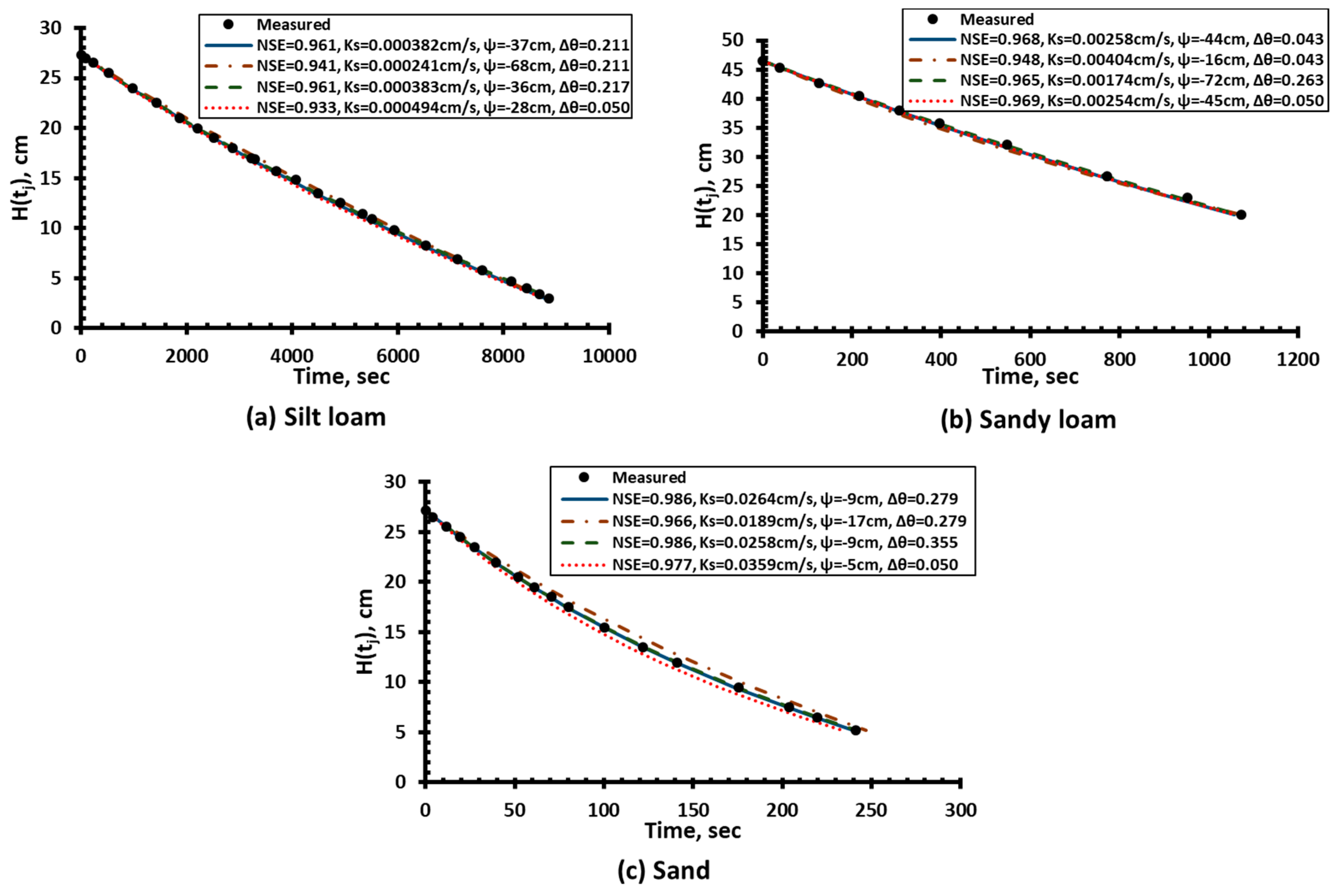
Figure 4 shows that the saturated hydraulic conductivity K_s is strongly correlated with the NSE but the Green–Ampt suction head Ψ at the wetting front is not. The highest NSE values for the most optimal set of parameters are 0.961, 0.968, and 0.986 for silt loam, sandy loam, and sand, respectively. An NSE threshold was adopted to delineate the successful sets of parameters (Figure 5) that produce the drawdown curve matching well with the observed drawdown data. The NSE threshold were determined as a ratio (0.98 was used in this study) of the highest NSE values of the most optimal set of parameters. The selected NSE thresholds were checked and show a well matching with the field-measured drawdown data for all the three types of soil (Figure 5). Please note that we have not used a fixed NSE (e.g., 0.9 or 0.95) as threshold to identify the successful sets of parameters since NSE also depends on which variable (e.g., $\Delta t_j$ or $\Delta H_j)$ is used to compute NSE (see Section 3.3), and the range between the highest NSE and the fixed threshold may vary for each test based on the value of the highest NSE.

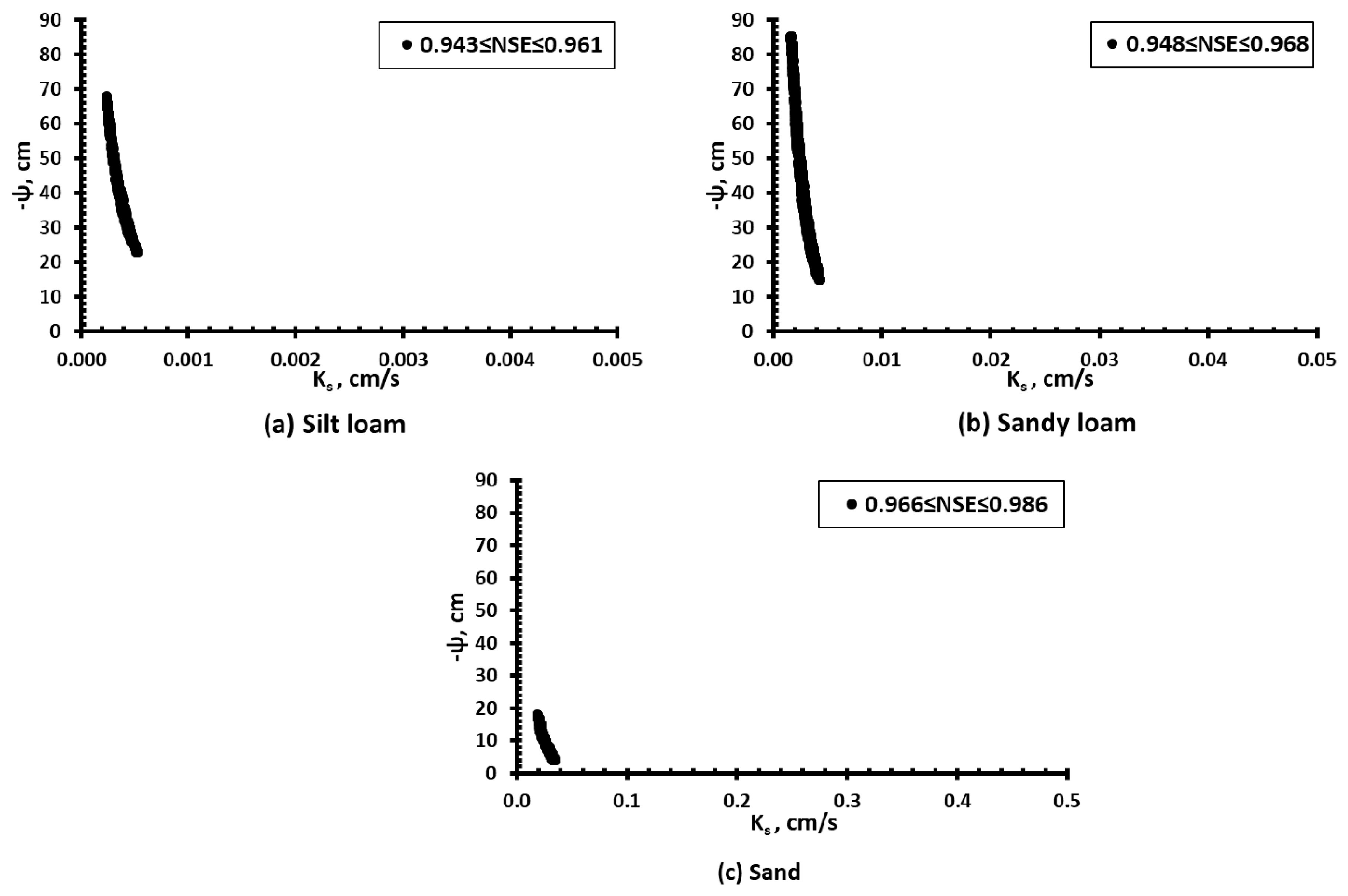
The successful values of K_s (with NSE ≥ the threshold) are ranged within the same order of magnitude that are consistent with the tested soil texture class: 2.4–5.3 × 10⁻⁴ cm/s, 1.6–4.3 × 10⁻³ cm/s, and 1.9–3.5 × 10⁻² cm/s for silt loam, sandy loam, and sand, respectively (Figure 6). Previous studies have shown that the measured K_s values may vary among the measurement methods by two or more orders of magnitude [26,44].

On the other hand, the successful Ψ (with NSE ≥ the threshold) values do not converge to a specific range as in the case of K_s. The Ψ values ranged between −68 cm and −23 cm, −85 cm and −15 cm, and −18 and −4 for silt loam, sandy loam, and sand, respectively (Figure 6). The successful sets of parameters K_s and Ψ (with NSE ≥ the threshold) for the three types of soil are plotted together in Figure 6.

The most optimal set of parameters (with the highest NSE values) determined using Application 2 and 3 (see Section 3.3) are reported in

Table 3. The most optimal sets of K_s and Ψ (with the highest NSE values) determined using Application 2 and 3 as described in the flowchart (see Figure 2) with measured Δθ, H_in, θ_in, and θ_s (input data) for the three tested soils (silt loam, sandy loam, and sand).

Soil Type	Hin	θin	θs	Δθ	Ks (cm/s)		Ψ (cm)
	(cm)				Application 2	Application 3	Application 2	Application 3
Silt loam	31.0	0.238	0.449	0.211	3.82 × 10−4	3.88 × 10−4	−37	−36
Sandy loam	51.0	0.339	0.382	0.043	2.58 × 10−3	2.83 × 10−3	−44	−37
Sand	33.5	0.096	0.375	0.279	2.64 × 10−2	2.74 × 10−2	−9	−8

. Using the backward-fitting analysis procedure introduced by Ahmed et al. [2], the fitted optimal parameters of K_s and Ψ using $\Delta {\mathrm{t}}_{\mathrm{j}}$ are 3.96 × 10⁻⁴ cm/s and −37 cm for silt loam with NSE of 0.961; 2.59 × 10⁻³ cm/s and −44 cm for sandy loam with NSE of 0.968; and 2.66 × 10⁻² cm/s and −9 cm for sand with NSE of 0.986.

Please note that all the synthetic drawdown data that were developed following the procedure of Application 1 (data of Figure 3) were also used in the sensitivity analysis procedure, which uses the forward-modeling code for Application 2 as described in the flowchart (see Figure 2). Results were similar to Figure 4, Figure 5 and Figure 6 determined using the measured drawdown data described earlier in this section.

3.3. Example of the Use of Application 3: Simulation Using $\Delta H_s\left(t_j\right)$ Determined by Equation (5) and Compare with the Changes in Measured Head Values $\Delta H\left(t_j\right)$

The collected data for the three types of soil were also analyzed using the forward-modeling code of the Application 3 mode (see Figure 2), which is based on estimating $\Delta {\mathrm{H}}_{\mathrm{s}}\left({\mathrm{t}}_{\mathrm{j}}\right)$ determined by Equation (5) and comparing with measured head changes, $\Delta \mathrm{H}\left({\mathrm{t}}_{\mathrm{j}}\right)$ values. Figure 7 shows the results out of the 30,000 sets of randomly generated parameters K_s and Ψ with corresponding NSE values greater than zero for the three types of soil. The number of parameter sets with NSE > 0 are 1.8%, 12.5%, and 5.0% of the 30,000 sets of the parameters for silt loam, sandy loam, and sand, respectively.

Results from the simulation using ∆H supported the strong correlation between NSE and K_s and the weak correlation with Ψ. The highest NSE values for the most optimal set of parameters are 0.914, 0.872, and 0.940 for silt loam, sandy loam, and sand, respectively. The NSE threshold was determined using the same ratio (0.98) of the highest NSE value applied in Section 3.2. Please note that the NSE calculated from ∆H is lower than the NSE calculated from ∆t. This difference comes from the definition of the NSE proposed by Nash and Sutcliffe [37] that is equal to one minus the sum of the absolute squared differences between predicted and observed values normalized by the variance of observed values. The variance of observed $\Delta H_j$ is typically less than the variance of $\Delta t_j$ (see Figure 3 and Figure 5); therefore, it leads to a lower value of NSE when NSE was determined using $\Delta H_j$.

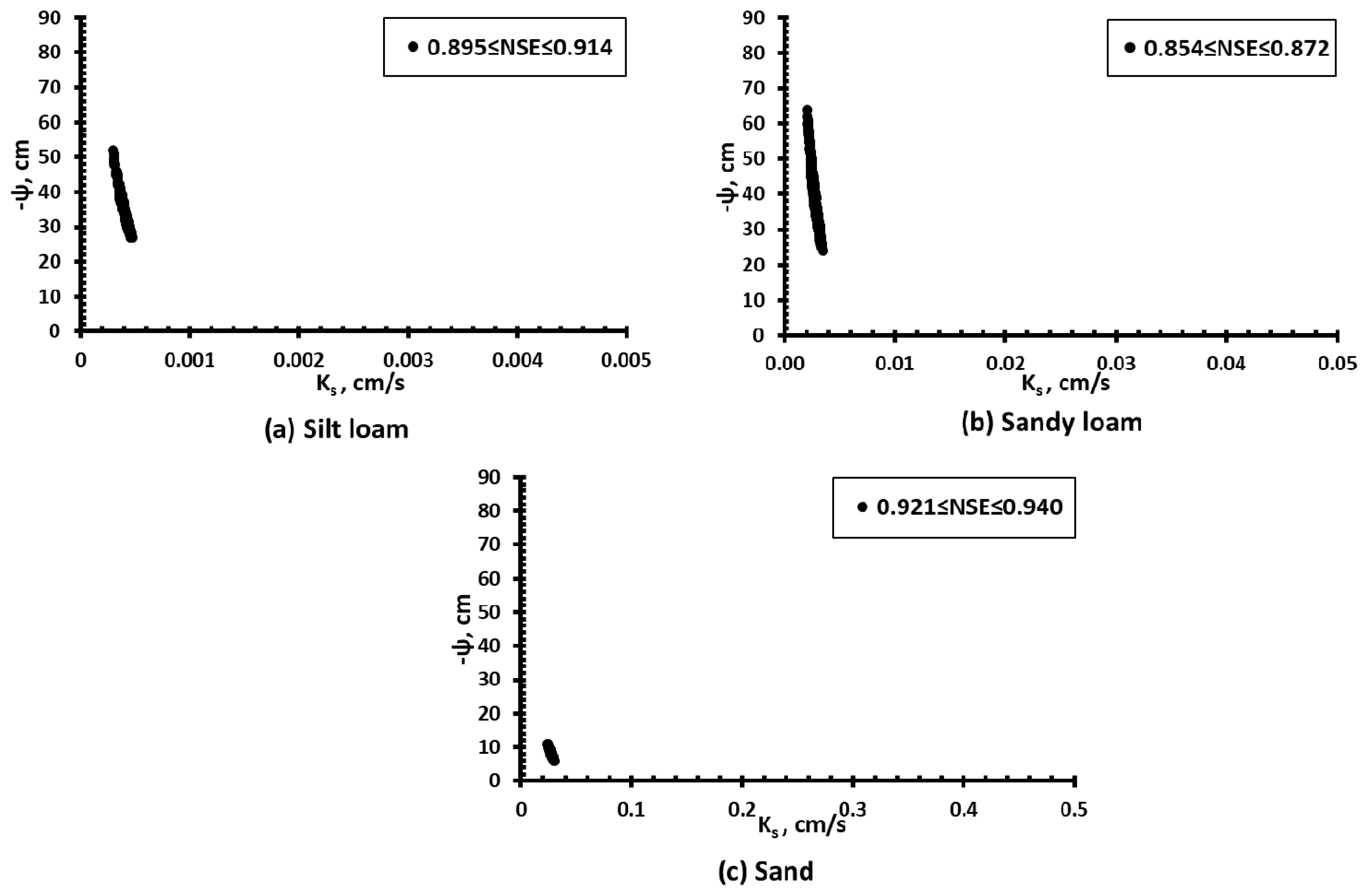
Similar to the results from Section 3.2, the successful values of K_s (with NSE ≥ the threshold) were ranged within the same order of magnitude that are consistent with the tested soil texture class: 2.9–4.7 × 10⁻⁴ cm/s, 2.0–3.5 × 10⁻³ cm/s, and 2.4–3.0 × 10⁻² cm/s for silt loam, sandy loam, and sand, respectively (Figure 8). The successful values of Ψ (with NSE ≥ the threshold) still do not converge to a specific range as in the case of K_s. The successful values of Ψ (with NSE ≥ the threshold) ranged between −52 cm and −27 cm, −64 cm and −24 cm, and −11 and −6 for silt loam sandy loam, and sand, respectively (Figure 8).

The most optimal set of parameters (with the highest NSE values) determined using Application 3 are reported in Table 3. Using the analysis procedure introduced by Ahmed et al. [2], the backward-fitted optimal parameters of K_s and Ψ using $\Delta H_j$ are 3.88 × 10⁻⁴ cm/s and −37 cm for silt loam with NSE of 0.914; 2.80 × 10⁻³ cm/s and −38 cm for sandy loam with NSE of 0.872; and 2.7 × 10⁻² cm/s and −8 cm for sand with NSE of 0.940.

3.4. Effects of Applying Varying Moisture Deficit Δθ on the Back-Fitted K_s and Ψ

Results from Figure 3 show that the drawdown curve predicted using the MPDI theory is different under varying soil moisture deficit ∆θ when Ψ is changed with θ_in. To examine the sensitivity of the MPDI to varying ∆θ, the soil properties K_s and Ψ were back-fitted using the measured drawdown data for silt loam, sandy loam, and sand using different ∆θ values including the maximum ∆θ_max and a very low ∆θ of 0.05 and the results are summarized in

Table 4. Values of the back-fitted saturated hydraulic conductivity K_s and the Green–Ampt suction head Ψ at the wetting front for silt loam, sandy loam, and sand using different moisture deficits Δθ.

Soil Type	Δθ	Ks	Ψ	H(t1)	NSE
		(cm/s)	(cm)	(cm)
Silt loam	0.211 (measured)	3.96 × 10−4	−37	27.4	0.961
	0.217 (maximum)	3.82 × 10−4	−37	27.3 a	0.961
	0.050 (assumed)	4.94 × 10−4	−28	30.2	0.933
	$\Delta {\theta }_{max}/4$ (assumed)	4.91 × 10−4	−28	30.1	0.934
	$\Delta {\theta }_{max}/2$ (assumed)	4.06 × 10−4	−35	29.2	0.966
	$3\Delta {\theta }_{max}/4$ (assumed)	3.95 × 10−4	−36	28.2	0.965
Sandy loam	0.043 (measured)	2.59 × 10−3	−44	50.3	0.968
	0.222 (maximum)	1.79 × 10−3	−70	47.2 a	0.965
	0.050 (assumed)	2.54 × 10−3	−45	50.2	0.969
	$\Delta {\theta }_{max}/4$ assumed)	2.51 × 10−3	−46	50.1	0.964
	$\Delta {\theta }_{max}/2$ (assumed)	2.21 × 10−3	−53	49.1	0.965
	$3\Delta {\theta }_{max}/4$ (assumed)	2.08 × 10−3	−57	48.2	0.964
Sand	0.279 (measured)	2.64 × 10−2	−9	28.8	0.986
	0.355 (maximum)	2.58 × 10−2	−9	27.5 a	0.986
	0.050 (assumed)	3.59 × 10−2	−5	32.7	0.977
	$\Delta {\theta }_{max}/4$ (assumed)	3.40 × 10−2	−5	32.0	0.961
	$\Delta {\theta }_{max}/2$ (assumed)	2.88 × 10−2	−8	30.5	0.986
	$3\Delta {\theta }_{max}/4$ (assumed)	2.78 × 10−2	−8	29.0	0.986

Note: ^a Minimum H(t₁) at Δθ_max that is used in Figure 5.

. Figure 5 shows that the simulated drawdown curves with the back-fitted K_s and Ψ using the maximum and a small ∆θ match well with the observed drawdown data for three types of soil. The back-fitted K_s and Ψ determined using different assumed ∆θ values are basically the same as the back-fitted K_s and Ψ using measured ∆θ if one considers their variations determined in the laboratory or the field. This means that the back-fitted K_s and Ψ using all the drawdown data are not sensitive to ∆θ, which is the same conclusion obtained by Regalado et al [45] using the Philip–Dunne permeameter; they only measured two infiltration times when the permeameter was half full and empty. This does not mean that the Modified Philip–Dunne drawdown curves are not sensitive to the initial moisture contents, as indicated by Figure 3.

Therefore, the user of the MPDI may assume/estimate ∆θ based on the field condition (wet or dry) to determine K_s and Ψ with a good accuracy if the user did not measure θ_in and/or θ_s since the moisture content θ values at the field capacity (for the lowest θ_in) and saturated condition are available for many reference books. For example, ∆θ can be set at 0.05, $\Delta {\theta }_{max}/4$, $\Delta {\theta }_{max}/2$, $3\Delta {\theta }_{max}/4$, and ∆θ_max depending on the observed wet to dry soil condition (Table 4). It is important to note that the same measured drawdown data of each type of soil were used to back-fit K_s and Ψ reported in Table 4 under different assumed ∆θ values.

4. Conclusions

We have developed a forward model that was used to further our understanding of the fundamentals of the MPDI theory and identify some of its advantages and limitations. The forward model can be used to simulate synthetic drawdown curves that describe the changes in the water height H(t_j) with time t_j when the values of K_s and Ψ are known. These simulation results can be used to design the MPDI surveys under different types of field conditions. The forward model can also be used later to determine K_s and Ψ values by fitting the synthetic drawdown data against field-measured drawdown data. In this study, the model was used in this curve fitting mode to evaluate the quality of fit of 30,000 sets of randomly generated values of K_s and Ψ against the field-measured drawdown datasets compiled for three types of soil. Results show that the model is highly nonlinear and therefore it does not yield a unique best fit. There are multiple sets of parameters that can be used to fit the field-measured drawdown data equally well. The quality of the fit is quantified using an NSE threshold value. Our results show that for the good fits (which are delineated by NSE ≥ the threshold value), the predicted values of K_s are within the expected order of magnitude value for the tested soil. However, the value of Ψ can vary considerably even for good fits, especially for soils with low K_s. Based on these results, we conclude that the MPDI is a useful method to estimate K_s but not a robust method to estimate Ψ. This finding is similar to the results from Gómez et al. [24] who also recommended to use alternate approaches to estimate the Green–Ampt suction head Ψ at the wetting front rather than using the Philip [18] method. In addition, we found that the model fitted K_s and Ψ values are not sensitive to the assumed value of the moisture deficit ∆θ, therefore, the user of the MPDI can estimate ∆θ based on qualitative field observations (i.e., wet or dry soil). For example, ∆θ can be set at 0.05 for wet soils, and $\Delta {\theta }_{max}/4$, $\Delta {\theta }_{max}/2$, $3\Delta {\theta }_{max}/4$, or Δθ_max for different levels of partially dry to fully dry soils, respectively. Further studies are needed to simplify the current MPDI theory to fit only the K_s values when Δθ and Ψ values are known, or to improve the experimental procedures that can yield more sensitive datasets that can help uniquely identify K_s and Ψ values.

References

- Kanwar, R.S.; Rizvi, H.; Ahmed, M.; Horton, R.; Marley, S.J. Measurement of field-saturated hydraulic conductivity by using Guelph and velocity permeameters. Trans. ASAE 1990, 32, 1885–1890. [Google Scholar] [CrossRef]
- Ahmed, F.; Nestingen, R.; Nieber, J.; Gulliver, J.; Hozalski, R. A Modified Philip–Dunne Infiltrometer for Measuring the Field-Saturated Hydraulic Conductivity of Surface Soil. Vadose Zone J. 2014, 13. [Google Scholar] [CrossRef]
- Mohanty, B.; Kanwar, R.S.; Everts, C. Comparison of saturated hydraulic conductivity measurement methods for a glacial-till soil. Soil Sci. Soc. Am. J. 1994, 58, 672–677. [Google Scholar] [CrossRef]
- Alagna, V.; Bagarello, V.; Di Prima, S.; Iovino, M. Determining hydraulic properties of a loam soil by alternative infiltrometer techniques. Hydrol. Process. 2016, 30, 263–275. [Google Scholar] [CrossRef]
- Reynolds, W.; Bowman, B.; Brunke, R.; Drury, C.; Tan, C. Comparison of tension infiltrometer, pressure infiltrometer, and soil core estimates of saturated hydraulic conductivity. Soil Sci. Soc. Am. J. 2000, 64, 478–484. [Google Scholar] [CrossRef]
- Alakayleh, Z.; Clement, T.P.; Fang, X. Understanding the Changes in Hydraulic Conductivity Values of Coarse-and Fine-Grained Porous Media Mixtures. Water 2018, 10, 313. [Google Scholar] [CrossRef]
- Sällfors, G.; Öberg-Högsta, A.-L. Determination of hydraulic conductivity of sand-bentonite mixtures for engineering purposes. Geotech. Geol. Eng. 2002, 20, 65–80. [Google Scholar] [CrossRef]
- Komine, H. Theoretical equations on hydraulic conductivities of bentonite-based buffer and backfill for underground disposal of radioactive wastes. J. Geotech. Geoenviron. Eng. 2008, 134, 497–508. [Google Scholar] [CrossRef]
- Sivapullaiah, P.; Sridharan, A.; Stalin, V. Hydraulic conductivity of bentonite-sand mixtures. Can. Geotech. J. 2000, 37, 406–413. [Google Scholar] [CrossRef]
- Francisca, F.M.; Glatstein, D.A. Long term hydraulic conductivity of compacted soils permeated with landfill leachate. Appl. Clay Sci. 2010, 49, 187–193. [Google Scholar] [CrossRef]
- Abeele, W. The influence of bentonite on the permeability of sandy silts. Nucl. Chem. Waste Manag. 1986, 6, 81–88. [Google Scholar] [CrossRef]
- ASTM-D5084-16a. Standard Test Methods for Measurement of Hydraulic Conductivity of Saturated Porous Materials Using a Flexible Wall Permeameter; American Society for Testing and Materials: Philadelphia, PA, USA, 2016.
- Lee, D.; Elrick, D.; Reynolds, W.; Clothier, B. A comparison of three field methods for measuring saturated hydraulic conductivity. Can. J. Soil Sci. 1985, 65, 563–573. [Google Scholar] [CrossRef]
- Wessolek, G.; Plagge, R.; Leij, F.; Van Genuchten, M.T. Analysing problems in describing field and laboratory measured soil hydraulic properties. Geoderma 1994, 64, 93–110. [Google Scholar] [CrossRef]
- Mallants, D.; Jacques, D.; Tseng, P.-H.; van Genuchten, M.T.; Feyen, J. Comparison of three hydraulic property measurement methods. J. Hydrol. 1997, 199, 295–318. [Google Scholar] [CrossRef]
- Reynolds, W.D.; Elrick, D.E. A Method for Simultaneous In Situ Measurement in the Vadose Zone of Field-Saturated Hydraulic Conductivity, Sorptivity and the Conductivity-Pressure Head Relationship. Groundw. Monit. Remediat. 1986, 6, 84–95. [Google Scholar] [CrossRef]
- Bagarello, V.; Iovino, M.; Elrick, D. A simplified falling-head technique for rapid determination of field-saturated hydraulic conductivity. Soil Sci. Soc. Am. J. 2004, 68, 66–73. [Google Scholar] [CrossRef]
- Philip, J. Approximate analysis of falling-head lined borehole permeameter. Water Resour. Res. 1993, 29, 3763–3768. [Google Scholar] [CrossRef]
- ASTM-D8152-18. Standard Practice for Measuring Field Infiltration Rate and Calculating Field Hydraulic Conductivity Using the Modified Philip Dunne Infiltrometer Test; American Society for Testing and Materials: Philadelphia, PA, USA, 2018.
- Merva, G. The velocity permeameter technique for rapid determination of hydraulic conductivity in situ. In Proceedings of the 3rd Workshop on Land Drainage, Columbus, OH, USA, 7–11 December 1987. [Google Scholar]
- Perroux, K.; White, I. Designs for Disc Permeameters. Soil Sci. Soc. Am. J. 1988, 52, 1205–1215. [Google Scholar] [CrossRef]
- Bouwer, H. Measuring Horizontal and Vertical Hydraulic Conductivity of Soil With the Double-Tube Method 1. Soil Sci. Soc. Am. J. 1964, 28, 19–23. [Google Scholar] [CrossRef]
- Reynolds, W.; Elrick, D. Ponded infiltration from a single ring: I. Analysis of steady flow. Soil Sci. Soc. Am. J. 1990, 54, 1233–1241. [Google Scholar] [CrossRef]
- Gómez, J.; Giráldez, J.; Fereres, E. Analysis of infiltration and runoff in an olive orchard under no-till. Soil Sci. Soc. Am. J. 2001, 65, 291–299. [Google Scholar] [CrossRef]
- Connolly, R.D.; Silburn, D.M.; Ciesiolka, C.A.A.; Foley, J.L. Modelling hydrology of agricultural catchments using parameters derived from rainfall simulator data. Soil Tillage Res. 1991, 20, 33–44. [Google Scholar] [CrossRef]
- Muñoz-Carpena, R.; Regalado, C.M.; Álvarez-Benedi, J.; Bartoli, F. Field evaluation of the new Philip-Dunne permeameter for measuring saturated hydraulic conductivity. Soil Sci. 2002, 167, 9–24. [Google Scholar] [CrossRef]
- Nestingen, R.; Asleson, B.C.; Gulliver, J.S.; Hozalski, R.M.; Nieber, J.L. Laboratory Comparison of Field Infiltrometers. J. Sustain. Water Built Environ. 2018, 4, 04018005. [Google Scholar] [CrossRef]
- Zhang, R. Determination of soil sorptivity and hydraulic conductivity from the disk infiltrometer. Soil Sci. Soc. Am. J. 1997, 61, 1024–1030. [Google Scholar] [CrossRef]
- Weiss, P.T.; Gulliver, J.S. Effective saturated hydraulic conductivity of an infiltration-based stormwater control measure. J. Sustain. Water Built Environ. 2015, 1, 04015005. [Google Scholar] [CrossRef]
- García-Serrana, M.; Gulliver, J.S.; Nieber, J.L. Infiltration capacity of roadside filter strips with non-uniform overland flow. J. Hydrol. 2017, 545, 451–462. [Google Scholar] [CrossRef] [Green Version]
- Kristvik, E.; Kleiven, G.H.; Lohne, J.; Muthanna, T.M. Assessing the robustness of raingardens under climate change using SDSM and temporal downscaling. Water Sci. Technol. 2018, 77, 1640–1650. [Google Scholar] [CrossRef] [PubMed]
- Taguchi, V.J.; Carey, E.S.; Hunt III, W.F. Field Monitoring of Downspout Disconnections to Reduce Runoff Volume and Improve Water Quality along the North Carolina Coast. J. Sustain. Water Built Environ. 2018, 5, 04018018. [Google Scholar] [CrossRef]
- Nestingen, R.S. The Comparison of Infiltration Devices and Modification of the Philip-Dunne Permeameter for the Assessment of Rain Gardens. Master’s Thesis, University of Minnesota, Minneapolis, MN, USA, 2007. [Google Scholar]
- ASTM-D2216-10. Standard Test Methods for Laboratory Determination of Water (Moisture) Content of Soil and Rock by Mass; American Society for Testing and Materials: Philadelphia, PA, USA, 2010.
- ASTM-F1815-11. Standard Test Methods for Saturated Hydraulic Conductivity, Water Retention, Porosity, and Bulk Density of Athletic Field Rootzones; American Society for Testing and Materials: Philadelphia, PA, USA, 2011.
- Clapp, R.B.; Hornberger, G.M. Empirical equations for some soil hydraulic properties. Water Resour. Res. 1978, 14, 601–604. [Google Scholar] [CrossRef] [Green Version]
- Nash, J.E.; Sutcliffe, J.V. River flow forecasting through conceptual models part I—A discussion of principles. J. Hydrol. 1970, 10, 282–290. [Google Scholar] [CrossRef]
- Rawls, W.J.; Brakensiek, D.L.; Saxtonn, K. Estimation of soil water properties. Trans. ASAE 1982, 25, 1316–1320. [Google Scholar] [CrossRef]
- Brooks, R.H.; Corey, A.T. Properties of porous media affecting fluid flow. J. Irrig. Drain. Div. 1966, 92, 61–90. [Google Scholar]
- Philip, J. The theory of infiltration: 5. The influence of the initial moisture content. Soil Sci. 1957, 84, 329–340. [Google Scholar] [CrossRef]
- Gray, D.M.; Norum, D. The effect of soil moisture on infiltration as related to runoff and recharge. In Proceedings of the Hydrology Symposium No. 6 Soil Moisture, Saskatoon, SK, Canada, 15–16 November 1967. [Google Scholar]
- Ruggenthaler, R.; Meißl, G.; Geitner, C.; Leitinger, G.; Endstrasser, N.; Schöberl, F. Investigating the impact of initial soil moisture conditions on total infiltration by using an adapted double-ring infiltrometer. Hydrol. Sci. J. 2016, 61, 1263–1279. [Google Scholar] [CrossRef]
- Ahmed, F. Characterizing the Performance of a New Iniltrometer and Hydraulic Properties of Roadside Swales. Ph.D. Thesis, University of Minnesota, Minneapolis, MN, USA, 2014. [Google Scholar]
- Durner, W.; Lipsius, K. Determining Soil Hydraulic Properties. Encycl. Hydrol. Sci. 2005, 1021–1144. [Google Scholar] [CrossRef]
- Regalado, C.M.; Ritter, A.; Alvarez-Benedi, J.; Munoz-Carpena, R. Simplified method to estimate the Green–Ampt wetting front suction and soil sorptivity with the Philip–Dunne falling-head permeameter. Vadose Zone J. 2005, 4, 291–299. [Google Scholar] [CrossRef]
Figure 1.
Notations used in the governing equations of the Modified Philip–Dunne Infiltrometer [33].
Figure 2.
Flowchart for the analysis procedure using the forward-modeling code used to generate the drawdown data and to estimate Ks and Ψ for values from measurements of head H(tj) versus time tj. Note: Between { } is the application number (e.g., Application 1, 2, and/or 3) that the corresponding parameter or a step is only used for that application/applications.
Figure 3.
Drawdown curves for (a) silt loam, (b) sandy loam, and (c) sand estimated by the forward-modeling code using the soil properties Ks and Ψ reported in Table 2 for two different values of Δθ representing wet and dry conditions. Three graphs (a–c) have different scales for the x-axis (time in sec).
Figure 4.
Scatter plots for the NSE calculated between determined by Equation (6) and the measured time intervals , on the left is NSE versus Ks (cm/s) and NSE versus - Ψ (cm) is on the right. (a) silt loam, (b) sandy loam, and (c) sand. The scales for Ks are different for each of the three soils.
Figure 5.
The field-measured and the simulated drawdown curves using the sets of parameters with the highest and threshold NSE values (determined using ∆t) and for Ks and Ψ back-fitted using two assumed ∆θ values: (a) silt loam, (b) sandy loam, and (c) sand. Note, the dots show measured drawdown data, the blue lines give the drawdown curves with the highest NSE (e.g., 0.961 for silt loam), and brown dash-dotted lines give the drawdown curves with the selected NSE threshold (e.g., 0.941 = 0.98 × 0.961 for silt loam).
Figure 6.
The successful sets of parameters Ks versus – Ψ (delineated by NSE ≥ the threshold value) determined from simulation using determined by Equation (6) and the measured time intervals : (a) silt loam, (b) sandy loam, and (c) sand. Note: The limits for Ks (or x-axis) are different for the three soils.
Figure 7.
Scatter plots for the NSE calculated between determined by Equation (5) and the changes in measured head , on the left is Ks versus NSE and −Ψ versus NSE is on the right. (a) Silt loam, (b) Sandy loam, and (c) Sand.
Figure 8.
The successful sets of parameters Ks versus - Ψ (delineated by NSE ≥ the threshold value) determined from simulation using determined by Equation (5) and the changes in measured head . (a) silt loam, (b) sandy loam, and (c) sand. Note: The limits for Ks (or x-axis) are different for the three soils.