SPH Modeling of Water-Related Natural Hazards

Abstract

This paper collects some recent smoothed particle hydrodynamic (SPH) applications in the field of natural hazards connected to rapidly varied flows of both water and dense granular mixtures including sediment erosion and bed load transport. The paper gathers together and outlines the basic aspects of some relevant works dealing with flooding on complex topography, sediment scouring, fast landslide dynamics, and induced surge wave. Additionally, the preliminary results of a new study regarding the post-failure dynamics of rainfall-induced shallow landslide are presented. The paper also shows the latest advances in the use of high performance computing (HPC) techniques to accelerate computational fluid dynamic (CFD) codes through the efficient use of current computational resources. This aspect is extremely important when simulating complex three-dimensional problems that require a high computational cost and are generally involved in the modeling of water-related natural hazards of practical interest. The paper provides an overview of some widespread SPH free open source software (FOSS) codes applied to multiphase problems of theoretical and practical interest in the field of hydraulic engineering. The paper aims to provide insight into the SPH modeling of some relevant physical aspects involved in water-related natural hazards (e.g., sediment erosion and non-Newtonian rheology). The future perspectives of SPH in this application field are finally pointed out.

1. Introduction

Thanks to the availability of high-performance computers, in the last few years, computational fluid dynamics (CFD) has been widely applied to simulate natural hazards in the field of hydraulic engineering. Due to the fast and large deformations characterizing the problems in this research field, meshless techniques allow for some intrinsic limitations of traditional grid-based methods (e.g., mesh deformation and cracking; free-surface, and interface treatment) to be overcome. Among the meshless techniques, the smoothed particle hydrodynamics (SPH) method has proven to have advantages over other methods. Following a Lagrangian approach, each continuum is discretized through a discrete set of material particles that lack connective mesh and follow the deformation undergone by the material. The dynamics of material particles obeys Newton’s laws of motion and the discretized form of the governing equations (i.e., momentum and mass balance) is obtained through particle approximation using an interpolant kernel function (i.e., a central function of the particles’ relative distance). Based on the solution algorithm of the discretized governing equations, two different approaches can usually be defined: weakly compressible SPH (WCSPH), if the continuum is assumed to be slightly compressible (governing equations can be decoupled), and incompressible SPH (ISPH).

Even if SPH was originally developed for astrophysical problems, it has been subsequently extended to the analysis of free-surface flows and several kinds of multiphase flows including non-Newtonian fluid and post-failure dynamics of rainfall induced landslide. Many works have shown that the multiphase coupled dynamics of water and non-cohesive sediment mixture may be simulated following a fluidic approach [1,2,3]. Through the proper definition of appropriate yielding criteria and non-Newtonian rheological models, the triggering and propagation of multiphase flow as well as dense rapid granular flow can be simulated through the SPH approach with a suitable degree of accuracy in reproducing the experimental results, showing that this approach can be conveniently applied to real case studies. In this way, it is possible to simulate scouring around complex structures that may cause hazards related to both structural instability and threats to the safe management of hydro-power plants [4,5,6,7]. Another important branch of non-cohesive sediment dynamics is related to two-phase flows on complex 3D topography such as the sediment eroded by a dam-break wave propagating on a mountain valley [8].

In the field of dense granular flows, fast landslide dynamics can be properly simulated by accounting for the interactions with water (both pore water and stored water) that influences landslide deformability and run-out characteristics. Thus, complex multiphase flows can be simulated for investigating natural hazard related to a tsunami wave generated by a quick landslide at the slope of a reservoir [9,10,11,12,13]. Additionally, a fast shallow landslide triggered by intense rainfall at the slope of a hill represents the most common natural hazards in some areas of the world [14,15] and can be simulated with proper numerical modeling. Furthermore, SPH can be successfully applied to the analysis of slope stability, with the detection of failure initiation and propagation leading to delineation of the potential slip surface [16].

Computational methods are also successful in simulating complex nonlinear flows and transport processes involved in natural hazards related to the flooding risk, as in the case of dam and dyke failures. Water wave propagation in complex 3D topography can be properly predicted [17,18,19,20] including urban areas where the complexity of the 3D flow pattern is increased by sudden changes in the propagation direction due to buildings as well as different types of floating bodies such as cars, trucks, etc., as in the works in [21,22].

Even if mathematical models have been widely established to simulate the relevant hydraulic and hydro-geologic processes involved in the simulation of water-related natural hazards [23,24,25], the relevant complexity (especially from a geometric point of view) of practical applications in the field of applied engineering poses some difficulties in the applications of the computer codes that implement the above-mentioned mathematical models. The numerical modeling of a complex 3D problem frequently requires the discretization of large domains with a high resolution, which implies simulating a very large number of elements (usually at least some millions), thus increasing the required computational time and resources in a non-linear way. Fortunately, the parallel computational power of the computer hardware has increased significantly in recent years, especially in the case of graphics processing units (GPUs) which are now several times more powerful than traditional central processing units (CPUs). However, it is important to note that the GPU is more powerful only for properly posed problems that are parallelizable on GPUs, and not necessarily for general computing. Furthermore, it is imperative that the models are implemented using high performance computing (HPC) techniques to take advantage of the power of current hardware (i.e., multi- cored CPUs, GPUs, or other hardware accelerators).

Another limitation that computational modeling suffers is the inherent uncertainties of some modeling parameters that influence (in some cases even significantly) the model response and lower the reliability of the results. Despite this intrinsic limitation, such deterministic models may be useful anyhow to support risk analysis and mitigation through the development of fast-running numerical models that can help to create probabilistic maps of risk variables. In this way, a multi-disciplinary decision support system for natural hazard risk reduction and management could be developed that allows for the exploration of several scenarios including potential risk-reduction options [26].

In this context, the aim of the paper was to provide an overview of some recent applications of the SPH method to the modeling of water-related natural hazards. The selected works illustrate some of the relevant problems of practical and theoretical interest in the field of hydraulic engineering that could be useful to provide an introduction to the SPH method as applied to the analysis and mitigation of water-related natural hazards.

Additionally, some widespread free and open-source software (FOSS) CFD codes for multiphase engineering applications are reviewed as well as their capabilities in modeling some of the problems described in this paper.

2. Two-Phase Coupled Dynamics

This section illustrates some engineering applications of the SPH method in the simulation of two-phase flows involved in hydraulic engineering problems of practical interest in the field of water-related natural hazards.

When dealing with the numerical simulation of two-phase flows of immiscible fluids, a central aspect to be considered is the interface treatment. Concerning incompressible SPH (ISPH) simulations of gravity currents induced by the inflow of a certain fluid into another fluid with a density difference, two different approaches were proposed in [27] and classified as a coupled model and a decoupled model, respectively. The coupled model is based on the assumption that standard ISPH governing equations can be applied to every particle in the computational domain regardless of the phase it belongs to. Therefore, when an interface particle is considered, the kernel interpolation is extended over all the heterogeneous neighbors in its interaction domain, which is the kernel compact support (circular in 2D problems or spherical in 3D problems) centered on the considered interface particle. In contrast, the decoupled model assumes that standard ISPH governing equations (including the Poisson equation) should be solved separately for each phase by identifying the free-surface. Therefore, if an interface particle is considered to be the kernel, interpolation is restricted to its homogeneous neighbors solely within the kernel support, thus kernel truncation occurs. Proper interface boundary conditions should be satisfied to couple both phases: these conditions can be represented by the continuity of both normal and tangential stresses between heterogeneous particles at the interface. According to the results in [27], the decoupled model also provides higher accuracy than the coupled model in the case of multi-fluid flow with a high-density ratio.

A modified formulation of the standard weakly compressible SPH (WCSPH) governing equations were presented in [28] for modeling rapid free-surface multiphase flows with a high-density ratio involving violent impact against a rigid wall. This formulation, which is based on the coupled approach, allows for the numerical instability induced by the discontinuity of the fluid properties across the interface to be eliminated without excluding the heterogeneous particle during kernel interpolation. Fairly accurate results were achieved with this coupled model simulating some flows with continuous pressure across the interface. Other good examples of multi-phase SPH formulations (both WCSPH and ISPH) that deal with the interface between fluids under certain constraints are described in the works in [29,30,31,32].

Among the variety of problems involving the numerical simulation of multi-phase flows, two topics of concern in the field of water-related natural hazards have been examined in the following: (i) scour with non-cohesive sediment transport induced by rapidly varied free-surface flow and erosion around complex structures; and (ii) fast dynamics of dense granular flows and landslides. Some relevant works on these topics are discussed, pointing out the peculiar aspects of numerical modeling.

2.1. Scouring and Sediment Transport

An important aspect of the design and maintenance of the bottom-founded submerged structure is non-cohesive sediment scouring. Bottom sediment erosion around the structure is caused by a complex flow pattern induced by the presence of the structure that strongly modifies the upstream undisturbed flow field [33]. The scouring evolution over time must be properly analyzed and mitigated in order to avoid worsening of structural stability due to foundation exposure.

This topic is widely investigated in fluvial hydraulics, in coastal areas, and in the marine environment. When dealing with a safety assessment of a hydraulic structure placed in the riverbed (e.g., bridges, barrages, etc.), the erosive action of the river stream must be reliably evaluated [34]. Several empirical formulas to predict final scouring are available, but the phenomenon is time-dependent and is affected by several uncertainties (related to both sediment and flow characteristics) as well as stochastic factors influencing the flow evolution such as transport and deposition of wood debris [5,35,36].

Additionally, in the design of highly demanding marine structures, the scour around the foundations should be dependably predicted [37,38]. For instance, a continuous one-way current due to the overtopping flow of an extreme tsunami wave may cause long-term erosion of the foundation on the rear side of the coastal protection structures [39,40]. Scour pit evolution behind the seawall induces the formation of eddies with increasing size to adapt the growing dimension of the scour cavity. Excessive sediment erosion directly results in the instability, and even destruction, of these hydraulic structures [41,42,43,44]. Most empirical relations have been established to predict the bulk and time-averaged sediment transport rate, but their application requires experimental data for calibration. Furthermore, these empirical relations were obtained from small scale laboratory experiments and their extension to a real scale problem may lead to significant erosion estimate errors [45].

An assessment of the mechanics of detailed temporal erosion processes as well as for the reliable design and assessment of these structures requires both physical investigations and advanced numerical modeling that accounts for the effects of the stochastic variables on the scouring process. Of course, numerical modeling is generally less expensive than physical experimentation, but, in some cases, experimental data may be available from technical literature. As with all engineering problems, any numerical tool must be properly validated against experimental data. After the model has been validated, its parameters require tuning based on the model/experiment results.

Many sediment modeling techniques use mesh-based approaches such as finite difference method and finite volume method to simulate the erosion and fluid-sediment coupled dynamics. However, these mesh-based methods suffer from some intrinsic limitations due to the fixed grid system, which leads to some difficulties in effectively simulating the bed-grain interactions, fluid-sediment momentum transmissions, and the dynamics within the deposits because of their fixed grid system. Furthermore, accurately tracking the free surface and fluid-sediment interface is also a big challenge for these approaches. Lagrangian meshfree particle methods overcome these limitations by intrinsically capturing the free-surface and tracking the particles. These methods have been widely used in recent years for the analysis of erosion processes.

The SPH technique has been proven to be effective in complex multiphase applications [46] such as water–gas flows or bubbly flow simulations [47,48]. In addition, when simulating non-cohesive bottom sediment scouring by rapid water flow, both weakly compressible (WCSPH) and incompressible (ISPH) formulations allow for a reliable description to be obtained. The basic idea is to model the sediment dynamics, likewise a pseudo-fluid, once the onset of sediment particle motion is attained. According to this approach, a criterion should be defined that represents the critical condition for the incipient motion of sediment; this can be done in terms of either critical velocity [49,50], or critical shear stress. The first approach may lead to some problems if critical velocity is evaluated as the depth-averaged value that in some cases may not be representative of the scouring, as for the continuous tsunami overflow behind a seawall that induces rapid water depth variation inside the scour pit [2]. The second approach based on the critical shear stress has been widely adopted to analyze non-cohesive sediment scouring by rapid water flows.

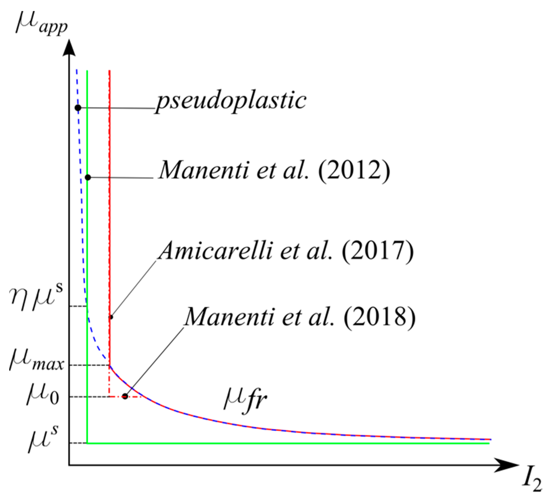
The authors in [7] implemented two different criteria in a WCSPH model to simulate the erosion process of non-cohesive bed sediment due to constant bottom water discharge from 2D tank (flushing). These criteria are based on Mohr–Coulomb (M–C) yielding theory and on Shields (SH) theory, respectively. The M–C critical condition defining sediment failure and the onset of erosion requires the introduction of a maximum viscosity as the product between sediment viscosity, μ_s, and a magnification factor, η, representing the numerical parameters to be tuned. When the apparent viscosity is lower than the maximum viscosity, the sediment is treated as a non-Newtonian fluid of Bingham type and solid particles are set in motion with constant viscosity μ_s (green curve in Figure 1). The strategy of introducing an upper viscosity limit for the sediment was also followed in [51] in the WCSPH simulation of complex problems in the field of marine engineering; below this maximum limit, the work in [51] adopted a variable apparent viscosity calculated through the M–C theory for the soil phase. The SH critical condition does not require the introduction of a numerical threshold for the viscosity of the solid phase. However, in [7], both the M–C and SH approaches require tuning of the mechanical parameters of the bottom sediment such as the angle of internal friction, φ, and sediment viscosity, μ_s, that became numerical parameters to fit the experimental eroded profile. This may be not be practical when calibration data are not available for the investigated problem.

In order to overcome this limitation, [8] proposed a WCSPH formulation of a mixture model for the analysis of dense granular flows consistent with the kinetic theory of granular flow (KTGF). This mixture model, which avoids the use of an erosion criterion, has been integrated into the FOSS code SPHERA v.9.0.0 (RSE SpA). The relevant physical properties (i.e., density and velocity) of the mixture of pure fluid and granular material are expressed as a function of the volume fraction ε, occupied by each phase at a material point. The balance equations for the mixture are defined accordingly and discretized consistently with the WCSPH approach. The frictional regime of the mixture dynamics is represented under the packing limit of the KTGF, which holds for the volume fraction ε_s of the solid (granular) phase and is characteristic of bed-load transport and fast landslides (see also Section 2.2). In the frictional regime, the mixture (or apparent) viscosity, μ, is calculated as a weighted sum of the pure fluid viscosity μ_f, and the frictional viscosity μ_fr, the latter being evaluated on the basis of the mean effective stress σ’_m, angle of internal friction φ, and the second invariant I₂ of the rate of the deformation tensor of the sediment. The frictional viscosity increases as the shear rate tends to zero, in accordance with the pseudo-plastic rheological behavior (dashed blue curve in Figure 1). To avoid the unbounded growth of apparent viscosity of the mixture, a threshold (or maximum) viscosity μ_max is introduced with a physical meaning. Threshold viscosity acts when approaching the zero shear rate; mixture particles with an apparent viscosity higher than the threshold viscosity are considered in the elastic–plastic regime of soil deformation where the kinetic energy of solid particles is relatively small and the frictional regime of the packing limit in the KTGF does not apply. For these reasons, the threshold viscosity is assigned to those particles that are excluded from the SPH computation (continuous red curve in Figure 1; below μ_max, the red curve coincides with the dashed blue curve of the pseudoplastic model). The excluded particles represent a fixed boundary with suitable values of the relevant physical properties and are included in the neighbor list of the nearby moving particle. The value of the threshold viscosity does not require tuning or calibration, but it should be selected for the specific problem; the value assigned to the threshold viscosity is the higher value that does not influence the numerical results significantly. Further increase of the value assigned to the threshold viscosity only affects the computational time because it determines an increase in the maximum value that can be assumed by the apparent mixture viscosity during the computation. The relationship between the mixture viscosity and the time step value that assures the stability of the adopted explicit time-stepping scheme is given by Equation 2.33 in [8]. When the numerical stability of the time integration scheme is dominated by the viscous criterion, the threshold viscosity reduces the computational time.

In [8], some experiments of erosional dam breaks adopting the physical values for the mechanical parameters of the sediments including the angle of internal friction were simulated with good reliability. The 2D experimental tests, involving rapidly varied mixture flows with erosion and the transport of bed sediment, were simulated in [7] and [8]. Moreover, in [6], mixture flow computation was performed with the open-source DualSPHysics solver [52] accelerated with a graphic processing unit (GPU). The adopted WCSPH algorithm, representing the improvement of the model in [53], reproduces the dynamics of the bottom sediment phase combining two erosion criteria with the non-Newtonian rheological model. The adopted rheological model is based on the Bingham-type Herschel–Bulkley–Papanastasiou (HBP) model providing the apparent viscosity μ_HBP of the sediment:

$${\mu }_{HBP}=\frac{\left|{\tau }_c\right|}{\sqrt{I_2}}\left(1-e^{-m\hspace{0.17em}\sqrt{I_2}}\right)+2\mu {\left(2\sqrt{I_2}\right)}^{n-1}$$

(1)

This model allows for the transition between un-yielded (fixed) and yielded (mobile) granular material to be described without introducing a maximum value of the viscosity for the solid phase. Proper selection of the HBP model’s parameters, m and n, allows for the reproduction of the required rheological behavior as the Newtonian or the pseudoplastic model. The yield stress parameter τ_c in the HBP model was evaluated in two different calibration procedures depending on the erosion criterion that holds for modeling the yielding mechanism of sediment. The qualitative representation of Equation (1) with n < 1 is denoted by the blue dashed curve in Figure 1.

If a solid particle is identified as being near the sediment–water interface by means of the criteria described in [6], then the Shields criterion determines the onset of bed erosion at the sediment–water interface and provides the critical bed shear stress τ_bcr, replacing the yield stress parameter τ_c, in the HBP model.

If the particle is near the water–sediment interface, but Shields erosion criterion is not satisfied or if the particle is far from the water–sediment interface, then the yielding mechanism is modeled through the Drucker–Prager criterion that allows the critical shear stress τ_y, replacing the yield stress parameter, τ_c, in the HBP model to be defined to determine the apparent viscosity for the sediment.

As a result, three distinct regions may be defined, starting from the water–sediment interface and going downward: (a) eroded sediment exceeding the Shields critical bed shear stress (bed load transport); (b) yielded sediment (plastic deformation with slow kinematics); and (c) un-yielded sediment (high viscosity, static condition).

The model proposed in [6] also accounts for suspended transport. Following [51], the identification of the suspension layer is obtained through a non-dimensional concentration, c_v, computed for an interface particle as the ratio of the sediment particle volume to the total particle volume within the interaction domain. The onset of suspended transport is determined by c_v falling below the threshold value of 0.3 and the suspended sediment viscosity is computed through [54] the experimental colloidal equation, which is more simple to implement with respect to the piece-wise function adopted in [51]. The density of suspended particles is computed by solving the mass balance equation. Even if, in some cases, the percentage gap between the experimental and numerically predicted maximum scouring depth is significant, it can be seen that the scour process is affected by several random factors and therefore reliable predictions of scouring effects are quite difficult to obtain, even with experimental modeling. The sediment dynamics models based on a synthetic rheological law (e.g., [6]) assume the same rheological behavior for the bed-load transport (frictional regime of KTGF), suspension for dense granular flows (kinetic-collisional regime of KTGF),a and suspension for diluted granular flows (kinetic regime of KTGF). This feature provides advantages and drawbacks with respect to KTGF-based sediment dynamics models (e.g., [8]). The model of [6] can reproduce several sediment transport regimes (not only bed-load transport), but is not coherent with KTGF, some parameters require tuning procedures, and non-transported granular material (e.g., landslides) is not treated.

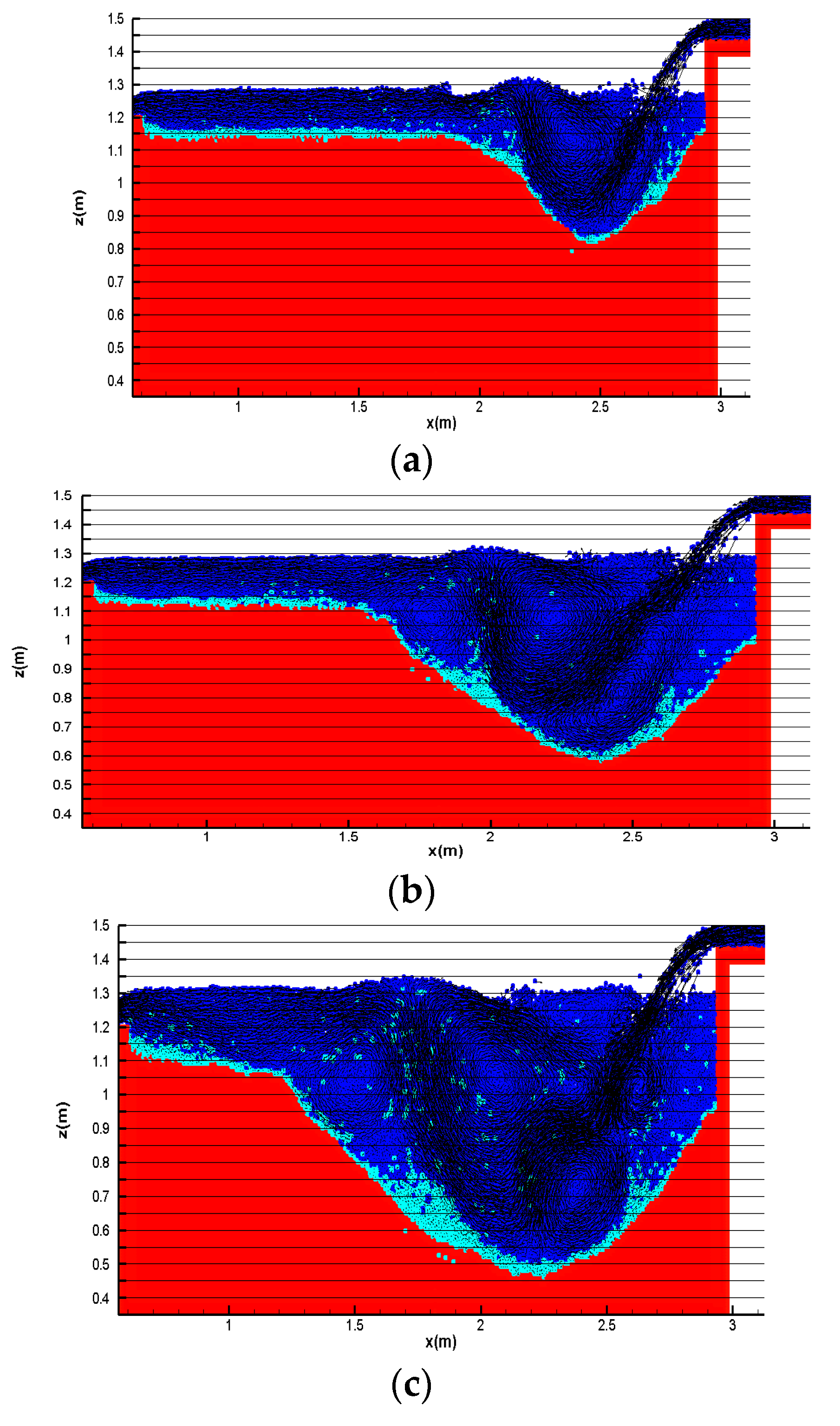
The work in [2] investigated by means of ISPH the water-induced 2D sediment scouring where the erosion process is mainly related to loose sediment particles suspended in the water flow, as in the case of scouring behind a seawall produced by continuous tsunami overtopping. In contrast to the physics of sediment flushing, where sediment moves as bed load at very high density, in the case of overtopping erosion, the solid particles move more loosely and the density of turbid water is significantly lower than the sediment density. In such situations, the erosion dynamics is controlled by the balance between the suspension effect due to turbulent mixing and settling of suspended solid particles owing to gravity force. This process is strongly affected by the size of numerical particles, which is usually far bigger than the size of a real sediment grain in practical problems. For the reasons explained above, adoption of real sediment density in the computation may lead to an unreliable representation of the erosion. The model proposed in [2] introduces a simplification due to the size (and hence number) of the particles required to properly model the turbulent mixing. This model is based on the concepts of numerical turbid water particle (TWP) and clear water particle (CWP) to simulate the sediment-entrained flow in cases where the granular particles of sediment move more loosely and sediment is washed away, mainly in the form of a suspended load. Due to the size considerations discussed above, numerical particles should be treated as a combination of clear water and turbid water particles if a suspended load is simulated; therefore, eroded solid particles represent a water–sediment mixture whose density is calculated based on the integral interpolation theory, thus accounting for density reduction as solid particles are suspended and mixed with water. The value of 1250 kg/m³ has been suggested for the reasonable initial density of the TWPs based on studies of bottom sediment movement. Figure 2 shows that the proposed ISPH model can simulate the real-time processes of the 2D overflow induced scouring. The detailed comparisons between numerical and experimental data can be found in [2].

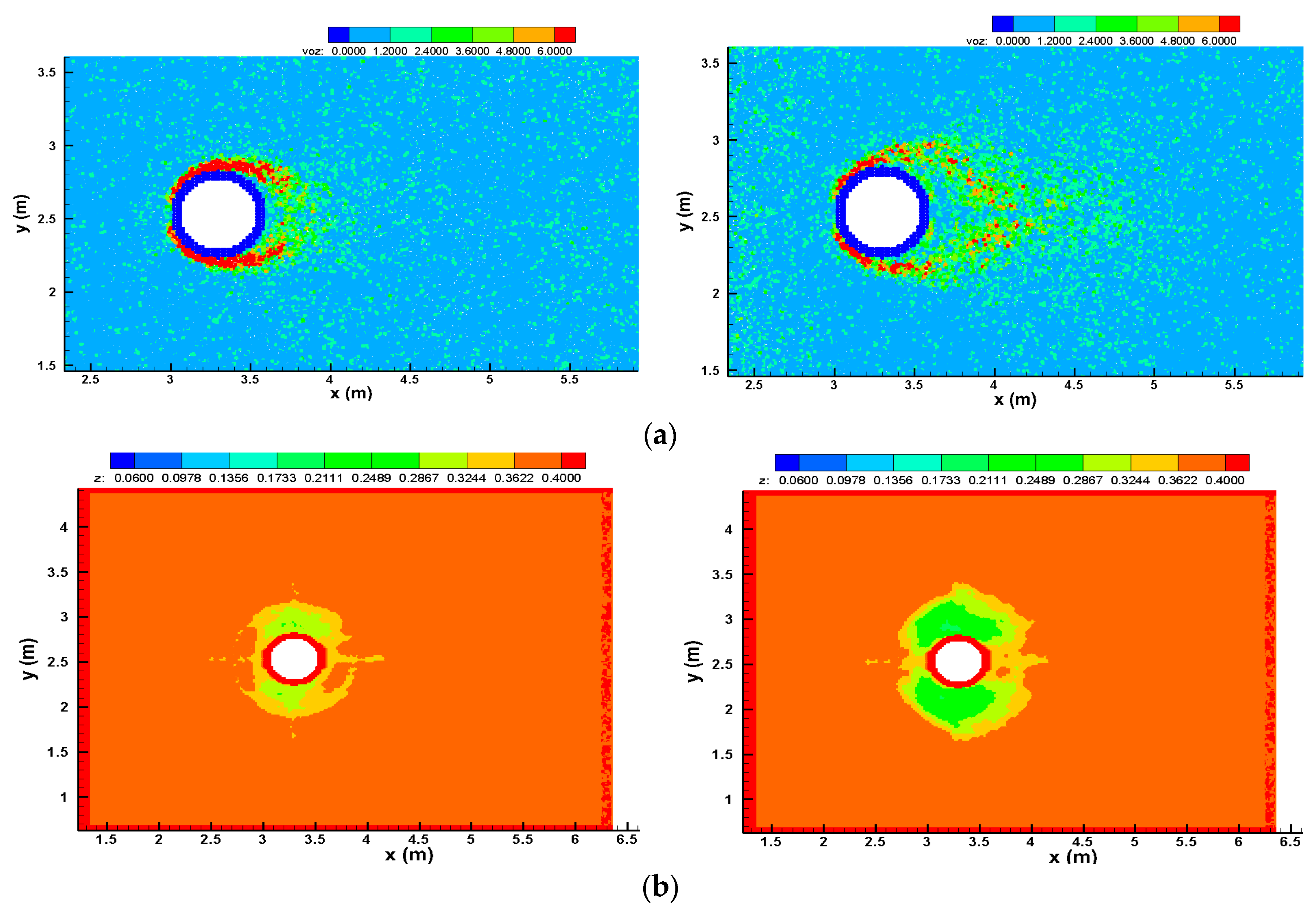
In the subsequent work in [1], the ISPH model of [2] was successfully extended to the simulation of 3D local bed scour induced by clear water stationary flow passing a submerged vertical cylinder of relatively large size. Additional formulations were introduced to account for transversal and longitudinal bed slope. The erosion model was based on the turbidity water particle concept and the sediment motion was initiated when the calculated shear stress on the interface particles exceeded the critical value. The 3D ISPH erosion model was used to simulate the scouring process around a large vertical cylinder with a diameter of 60 cm in Figure 3, where the vorticity and the shape of the scour pit are illustrated at time t = 2.5 s and t = 3.5 s. The numerical results show that the proposed ISPH model could simulate the relevant features of the flow and the scour process (Figure 3). The detailed comparisons between the numerical and experimental data can be found in [1] and the scour dynamics were validated with a suitable degree of accuracy for engineering purposes. Even if a suitable representation of the complex scouring process can be obtained, the vorticity field shows some numerical noise (Figure 3a). Improvement of the calculated vorticity field could be obtained through the approach proposed in [46].

2.2. Fast Landslides and Dense Granular Flows Interacting with Water

Numerical modeling of dense granular flows and landslides is still a challenging topic, especially when considering the interaction between the sediment and the water that may be both an internal interaction, related to pore water in landslide-prone saturated soil, and an external interaction with stored water in a basin with unstable slopes.

The interaction between pore water and soil matrix is a fundamental aspect that influences the triggering and propagation of shallow landslides induced by intense rainfall events that represent the most common natural hazards in some areas of the world [14]. Intense rainfall events induce water infiltration at slopes, leading to an increase of the volumetric water content and pore water pressure that worsen the slope stability of the soil layer close to the surface and may cause its failure. Reliable assessment of landslide susceptibility also requires a proper definition of the rainfall characteristics considering recent climate trends affecting rainfall [55,56].

If landslide triggering occurs, in the post-failure phase, the pore water content, combined with geo-mechanical properties of the soil, influence the sediment dynamics, and may induce in some cases flow-like fast earth movements classified as complex landslides because their run-out start as shallow rotational-translational failure, but changes into dense granular flows due to the large water content [15]. In this case, the fast landslide dynamics is more difficult to predict using traditional analytical models and a numerical approach could be helpful for landslide susceptibility assessment and the creation of debris–flow inundation maps.

The work in [57] proposed a combined triggering–propagation modeling approach for the evaluation of rainfall induced debris flow susceptibility. They adopted the transient rainfall infiltration and grid-based regional slope-stability model (TRIGRS) [58], which is based on the infinite slope stability approach, to obtain a map of potentially unstable cells within a study catchment under an intense rainfall event. Since not all unstable cells, in general, evolve to a debris flow, an empirical instability-to-debris-flow triggering threshold is calibrated on the basis of observed events and used to identify, among unstable cells, the so-called triggering cells that could most likely contribute to debris flow. The triggering threshold is, therefore, the key element that allows coupling between the TRIGRS slope instability model and the debris flow propagation model FLO-2D [59], a finite volume model that numerically solves the depth-integrated flow equations. The work in [57] assumed a zero excess rainfall intensity and a total friction slope depending on the Bingham-type rheological parameters as a function of the sediment concentration. The calibration of the triggering threshold with geo-morphological data of the catchment area represents a crucial step for obtaining reliable susceptibility maps in the nearby areas. Back-analysis of a catastrophic event that occurred on 1 October 2009 in the Peloritani mountain area (Italy) provided fairly good results.

In order to quantify the level of risk addressing the uncertainty inherent in landslide hazard, the susceptibility evaluation represents only one of the relevant issues involved in risk analysis. Additionally, run-out dynamics should be properly assessed in order to provide a quantitative estimate of the landslide hazard and select appropriate protective measures for risk mitigation. In order to reach such a goal, reliable predictive models should be used to obtain quantitative information on the destructive potential of the landslide. This is mainly related to the following characteristics: run-out distance; width of damage corridor; travel velocity; characteristic depth of the moving mass; and characteristic depth of the deposits [60].

The work in [61] proposed a 2D depth-integrated, coupled, SPH model for predicting the path, velocity, and depth of flow-like landslides. While the post-failure flow model of [57] assumes the heterogeneous moving mass as a single-phase continuum, [61] modeled the dense granular flow as a two-phase mixture composed of a solid skeleton with the voids filled by a liquid phase. Assuming that the shear strength of the liquid phase can be disregarded, the stress tensor within the mixture is composed of pore pressure and effective stress. Then, the mixture dynamics was described by quasi-Lagrangian depth integrated governing equations of mass and momentum balance, and the pore pressure dissipation equation that were discretized according to the standard SPH approach. Depth-integrated equations do not provide information on the vertical flow structure that is needed for evaluating shear stress on the bottom and depth integrated stress tensor. For this reason, [61] assumed that this vertical structure would be the same as the uniform steady-state flow according to the so-called model of the infinite landslide having constant depth and moving at a constant velocity on a constant slope. The work in [61] adopted the simple method proposed in [62] to obtain the bottom shear stress in a non-Newtonian fluid of Bingham-type. The model in [61] was used to simulate some catastrophic event that occurred on May 1998 in the Campania region (Italy), showing the relevant role of geotechnical parameters (especially the fluid phase and angle of internal friction) for the reliable prediction of the run-out distance, velocity, and height of the landslides. Proper selection of the value assigned to these parameters assured the best agreement with the field observations.

Some flow-like landslides are characterized by a relatively small average depth if compared with the horizontal linear dimensions, therefore the assumption of a depth-integrated model is strongly consistent with the physics of the phenomenon. Furthermore, there could be rainfall induced landslides where the initial average depth is comparable with the horizontal length and width. In these cases, significant variations of the vertical thickness and the vertical velocity profile may occur along the landslide body in the flow direction. This is illustrated in Figure 4, showing the preliminary results of an on-going study. In this new study, a narrow landslide that occurred during an intense rainfall event on April 2009 in a hilly area of the Oltrepò Pavese, named the Recoaro Valley, Northern Italy, was reproduced by means of the 2D WCSPH simulation. It can be seen that in the early phase, just after the failure, the mass portion close to the landslide front moved faster than the rear portion. Additionally, just after the impact against the downstream vertical wall of a damaged building, the landslide front began decelerating while the rear mass portion on the steep slope still maintained a relatively high average speed.

In the peculiar case described above, the modeling approach based on the infinite landslide with constant depth and moving at a constant velocity on a constant slope may be less appropriate. Therefore, the solution of the governing equation in the three-dimensional form seems more appropriate than the depth-integrated model. The simulation shown in Figure 4 was carried out with the code SPHERA v.9.0.0 adopting the mixture model for dense granular flow discussed in [8]. Even if the code has a 3D formulation, a 2D approach may be conveniently adopted in this case because the landslide is relatively narrow and the flow may be assumed to be identical on the vertical planes along the flow direction.

The work in [63] used a finite volume approach to simulate mudflows and hyper-concentrated flows characterized by suspended fine material by adopting a Bingham rheological model. Similar to [64], the Cross model was adopted for modeling the non-Newtonian flow, assuming that the constant parameter m was equal to 1, resulting in the following formulation of the apparent viscosity:

$$\begin{array}{l}{\mu }_{eff}=\frac{{\mu }_0+{\mu }_{\infty }\hspace{0.17em}K\hspace{0.17em}\dot{\gamma }}{1+K\hspace{0.17em}\dot{\gamma }}\\ K=\frac{{\mu }_0}{{\tau }_B}\hspace{1em}{\mu }_{\infty }={\mu }_B\end{array}$$

(2)

In Equation (2) $\dot{\gamma }$ denotes the shear rate defined through the second invariant I₂ of the rate of deformation tensor; K, μ₀, and μ_∞ are three constant parameters that can be conveniently related to common Bingham rheological parameters, namely the yield stress τ_B and viscosity μ_B. From a physical point of view, μ₀ and μ_∞ denote the viscosity at very low and very high shear rate, respectively. In order to avoid numerical divergence caused by the unbounded growth of effective viscosity as the shear rate approaches zero, μ_eff is limited to a suitably high threshold value, which is set to μ₀ = 103μ_B to assure convergence. The test cases simulated in work in [63] considered the flow on inclined surfaces and analyzed the role of the Froude number [65] during the propagation phase, which may be helpful in designing the control works.

Landslides occurring at the slopes of confined water bodies (e.g., artificial basin or river-valley reservoir) or at coastal regions involve complex interactions between the solid and the fluid phase. In the post-failure phase of rapid landslides generated at the slope of a water body, an impulse wave is generally induced, which is usually referred to as tsunami [66,67]. The characteristics of the generated water wave are related to the velocity and the shape (e.g., thickness and slope angle) of the landslide front, whose dynamic deformation is in turn affected by the water induced stresses at the interface while the landslide is penetrating the water body. Accurate prediction of the landslide induced wave hazard depends on reliable numerical models that can simulate the coupled dynamics.

The work in [11] proposed a WCSPH model for the analysis of impulsive wave generated in a basin by a deformable landslide. In order to properly reproduce landslide deformation during the post-failure phase, they adopted an elastic–plastic constitutive model for the soil combined with the Drucker–Prager criterion. To account for the interaction with stored water, occurring at a very small timescale due to the fast dynamics, [11] introduced a bilateral coupling model consisting of two sequential steps: the interface soil particles were initially considered as the moving deformable boundary whose velocity and position was used for solving the governing equations of the water phase; then the soil constitutive equation was solved with the corrected stress taking into account the water-induced surface force. This coupling model would require, in theory, an iterative procedure to assure the consistency of both stress and deformation at the interface at each time step. However, the sequential approach is quite suitable because the interface deformation is mainly caused by the landslide dynamics and small displacements occur within a time step. The mechanical parameters in the model of [11] have a physical meaning and the corresponding values can be deduced from conventional soil mechanic experiments. Two experiments were simulated concerning the wave generated by a slow landslide [12] and a fast landslide [68], respectively, obtaining in both cases good agreement with the experimental data.

The work in [10] proposed a hybrid model for simulating the coupled dynamics between the landslide and stored water as well as the propagation of generated surge waves. The discrete element method (DEM) was used for simulating the landslide dynamics, while WCSPH was used to solve the governing equations for water. Spurious numerical noise affecting the water pressure field was removed by applying the δ-SPH technique [69]. The interaction mechanism between the solid and fluid phase in the hybrid DEM-SPH model was based on the drag force and buoyancy. At each time step, these forces were first calculated considering (i) the initial position and velocity of both fluid and solid particles, (ii) the pressure of the fluid, and (iii) the local soil porosity, ε, evaluated at the landslide–water interface with a kernel interpolation of the solid particle volume. Based on the calculated drag force and buoyancy, the corresponding new position and velocity of both fluid and solid particles were then calculated to solve the corresponding discretized governing equations. The updated position and the velocity field were subsequently used to recalculate drag force and buoyancy. Therefore, this interaction mechanism requires an iterative process to assure convergence of the calculated forces and consistency of the displacements and velocity field of the involved phases. The hybrid DEM-SPH model was used to simulate the sliding along a 45° sloping plane of a rigid body that mimics a submarine landslide, obtaining a suitable prediction of the experimental time evolution of water surface elevation [70]. A modified simulation was additionally performed by considering the deformability of the sliding body, showing that smaller and less violent surge waves were generated owing to the landslide deformation.

A similar approach was proposed in [71] for the analysis of underwater granular collapse by coupling WCSPH (for the fluid phase) with DEM (for the solid incoherent phase). A coupling module was developed for fluid–grain interaction: the force exerted by the fluid on a solid particle was obtained by integrating the contributions on its surface; in turn, the effect of the solid particles on the fluid motion was calculated by including the neighboring DEM particles in the SPH interpolation of the governing equations for the considered liquid particle. Another attempt of coupling SPH, in particular, the DualSPHysics model, with a distributed-contact discrete-element method (DCDEM) was proposed in [72] to explicitly solve the fluid and solid phases to model a real case of an experimental debris flow. An experimental setup for stony debris flows in a slit check dam was reproduced numerically, where solid material was introduced through a hopper, assuring a constant solid discharge for the considered time interval.

The reference mixture model of [8] for the dynamics of dense granular flow was modified by introducing a numerical parameter, μ₀, referred to as limiting viscosity. The effect of limiting viscosity arises in the frictional regime at low deformation rates near the transition zone to the elastic–plastic regime: in this shear rate interval, a constant value μ₀ (lower than μ_max) is assigned to the mixture viscosity (see red dot-dashed curve in Figure 1), thus reducing the computational time in the case where the viscous criterion dominates the numerical stability of the time integration scheme. There are other alternative approaches to keep control of computational time in the simulation of high-viscosity flows. In the work of [73], a semi-implicit integration scheme was proposed to overcome the severe time-stepping restrictions caused by the WCSPH explicit integration scheme when simulating highly viscous fluids, as in the case of lava flow with thermal-dependent rheology. According to this approach, only the viscous part of the momentum equation is solved implicitly, thus saving computational time and obtaining an improved quality of the results with respect to the fully explicit scheme.

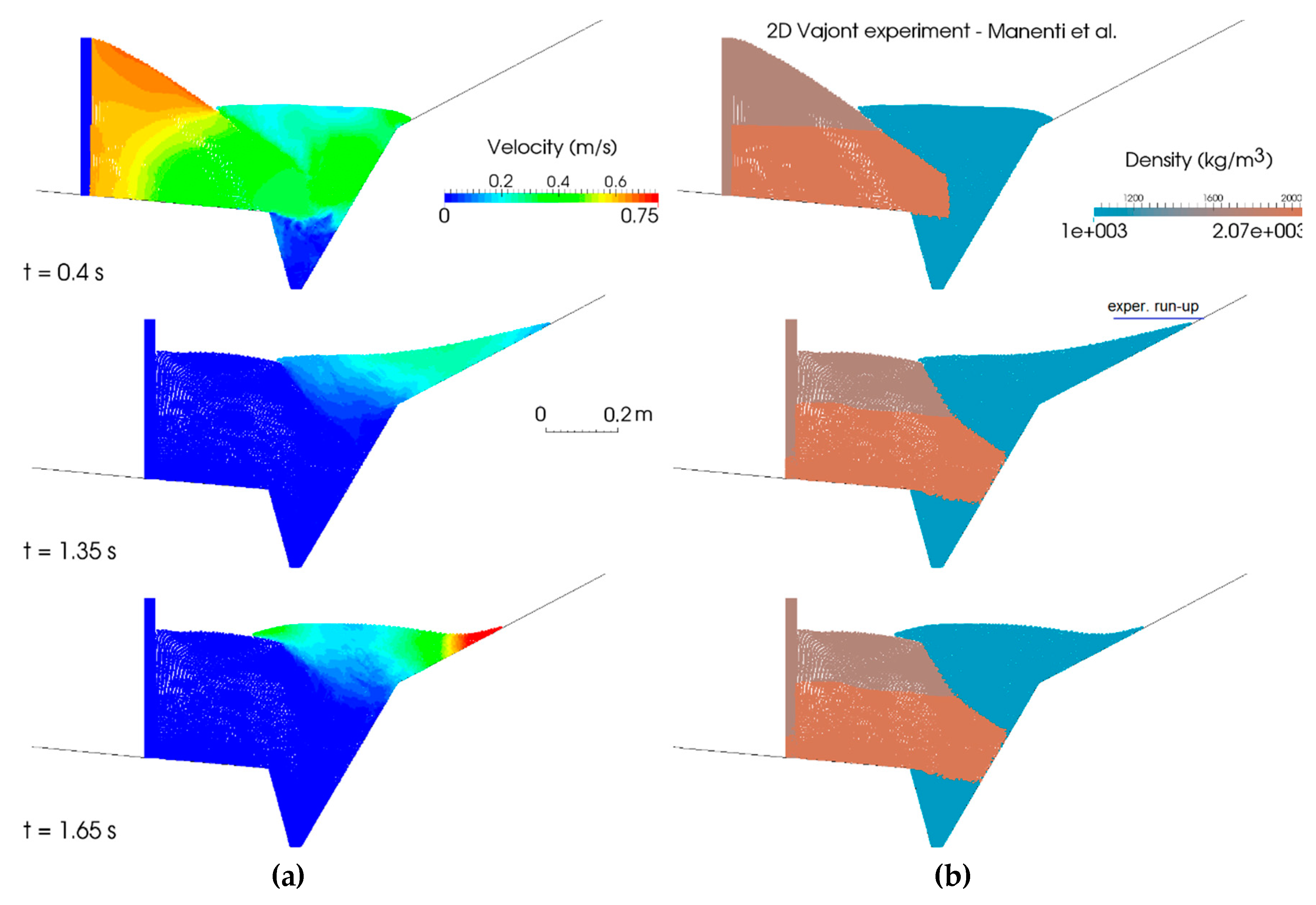
The mixture model of [8], modified with limiting viscosity, was successfully applied in [9] to the analysis of a fast massive landslide at the slope of an artificial reservoir. The simulated case reproduced a two-dimensional scale laboratory test carried out in 1968 at the University of Padua reproducing in Froude similitude a characteristic cross-section of the Vajont artificial basin. In 1963, a catastrophic landslide, estimated to be about 270 million cubic meters, fell into the Vajont reservoir, generating a tsunami that caused about 2000 casualties [74].

The experimental campaign of Padua aimed to evaluate the effects of both the material type and the landslide falling time on the maximum run-up of the generated wave over the opposite side of the valley. The landslide velocity was imposed through a rigid plate pulled by an engine through a steel cable. Several tests were carried out considering two types of rounded gravel (3–4 mm and 6–8 mm), crushed stone, and squared tile. For each of these material types, different values of the run-out velocity were tested by varying the plate stroke (in the range 0.5–0.8 m) and its velocity, thus resulting in a landslide falling time ranging approximately between 15 s and 500 s at full scale.

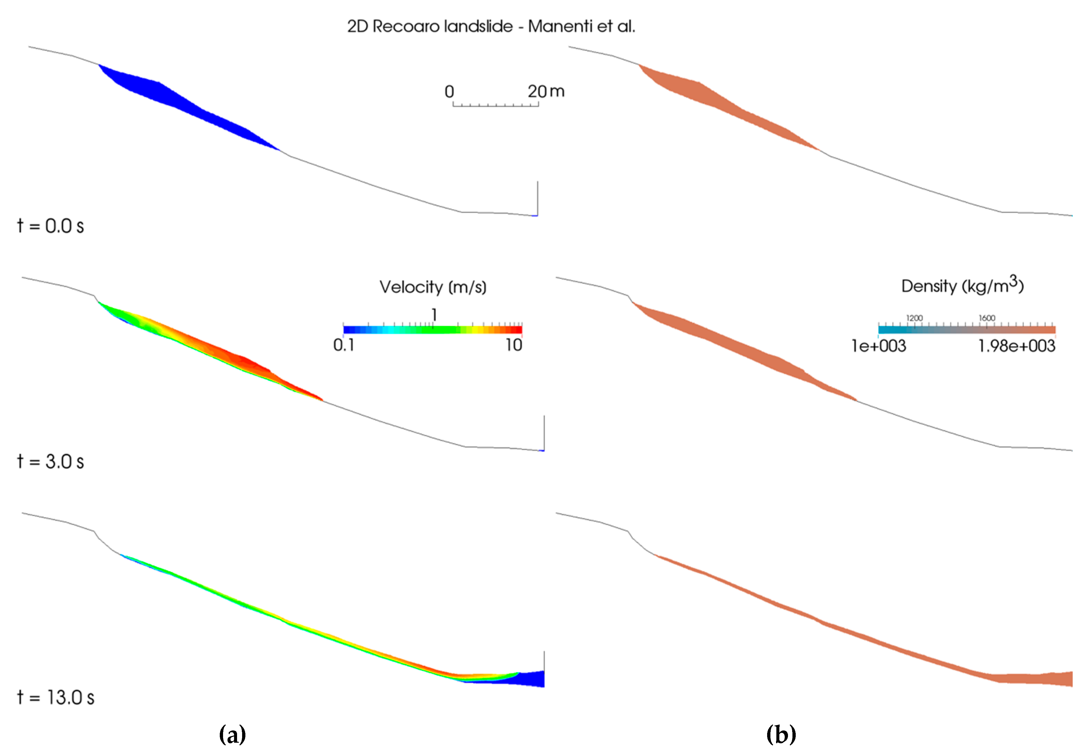
The frames in Figure 5 show the simulation results obtained with SPHERA v.9.0.0 [75]; some representative instants were selected during the acceleration phase where the vertical rigid plate pushes the landslide toward the basin, and the subsequent run-out phase of the generated wave climbs the opposite slope. Fairly good results were obtained in terms of the maximum height reached by the rising wave front. The left-hand panels show the velocity field evolution. The right-hand panels show the density field; it can be noticed that the lower landslide layer (light-brown) has a higher density because of the saturation. The effect of pore water allows for the landslide dynamics to be obtained more close to the experimental results because at t =1.35 s, its front comes into contact with the opposite side of the basin. No tuning of the physical parameters of the model was necessary. The required accuracy was controlled by the proper adoption of the limiting viscosity value, μ₀, reaching a reasonable compromise with consumed computational time. This test case is provided as tutorial number 35 in the documentation of SPHERA v.9.0.0 that is freely available in [76].

Calculation of the flow-impact induced forces on the submerged structure may be required in order to estimate landslide and water-related hazards. Using the standard WCSPH approach usually leads to high-frequency numerical noise in the pressure field [29] that may taint the calculation of the load time history acting on the solid structure. To overcome this problem and obtain the correct prediction of the hydrodynamic load for structural stability assessment, several strategies have been successfully introduced [77].

3. Flooding in Complex Topography with the Transport of Sediments

This section provides synthetic discussions on the following topics: state-of-the-art of CFD mesh-based codes for flood propagation on complex topography with sediment transport; advantages of SPH modeling for flood propagation on complex topography; state-of-the-art of SPH codes for sediment transport; example of a SPH code for flood propagation on complex topography with sediment transport; and pre-processing and post-processing tools for floods on complex topographies (i.e., real topographic surfaces or their scale models). The most popular codes used to represent erosional floods (i.e., flood propagation over granular beds) rely on mesh-based numerical methods and the shallow water equations (SWE). These are briefly recalled in the following. The work in [78] presents a finite element code for bed-load transport. A major novelty is the 3D mathematical formulation. However, the code validations only refer to 1D configurations in 2D domains where analytical solutions are available. The work in [79] introduced a Godunov-type 1D SWE model for 2D erosional dam-break floods. The work in [80] presented a 2D SWE-FVM (finite volume method) model for 3D erosional dam-break floods, which uses Exner’s equation for the bed top evolution, a 1D heuristic formula for the bed-load transport rate, and a 1D spatial reconstruction scheme based on Riemann solvers suitable for multi-phase flows. The work in [81] presented a 2D SWE model for 3D erosional dam-break floods; validations refer to 1D and 2D bed-load transport configurations, whereas a 3D demonstrative configuration (still represented with a 2D code) was reported on a quake-induced erosional dam-break flood (Tangjiashan Quake Lake). The work in [82] applied a 2D SWE-FVM code to simulate an erosional flood with bed-load transport in the Yellow River. The last two examples might represent typical applications of 2D SWE mesh-based models to 3D erosional floods on complex topography with 1D schemes for sediment transport.

The above mesh-based models share the following drawbacks: 2D modeling; no consistency with the KTGF; ad-hoc tuning procedure for the viscosity of the 2-phase mixture (water and granular material); and shallow-water approximation (e.g., hydrostatic pressure profiles, velocity is uniform along the vertical).

With respect to the above state-of-the-art mesh-based models, the meshless SPH numerical method introduces several advantages, which are synthesized in the following. SPH allows the detailed 3D fluid dynamics fields within the urban canopy (urban fabric) to be simulated including fluid-structure interactions, whilst the mesh-based 2D porous models do not provide a direct modeling of the flood-building interactions. The SPH method can simulate the 3D transport of solid structures and fluid interactions with other mobile and fixed structures and can also represent 3D bed-load transport and its impact on mobile and fixed solid structures. The SPH method provides a direct estimation of the position of the free surface and the fluid and phase interfaces due to its Lagrangian nature. The direct representation of Lagrangian derivatives is also responsible for the absence of the advective non-linear terms arising in the Eulerian formulation of the balance equations. No computational mesh generation is requested, thus saving person-months, software licenses, and computational resources. Nonetheless, several drawbacks have been reported. SPH is slightly more time consuming then mesh-based methods (fixed with the same spatial resolution and accuracy) and has a narrower, but peculiar range of application fields, whose number is nonetheless elevated and relevantly involve floods. Furthermore, a SPH code can usually cover a wide range of spatial resolutions at different accuracy levels, but maintain stable algorithms. This allows the same code to be used for both preliminary analyses at a coarse spatial resolution and accurate simulations (at fine spatial resolution).

Although several SPH studies are available for 2D and 3D applications for granular flows, only a few have been dedicated to floods with sediment transport (over a simplified topography). Among these studies, [7] introduced a 2D erosion criterion to represent the sediment removal from water bodies by means of discharge channels (i.e., flushing procedures). Regardless of the application, the SPH models for granular flows were mostly restricted to 2D codes, featured by either 2-phase models or ad-hoc tuning for mixture viscosity.

Recently, a numerical mixture model for dense granular flows was presented in [8] to simulate the sediment dynamics phenomena, which typically involve the failure of earth-filled dams and dykes, bed-load transport, and fast landslides over complex topography. This model is discussed in the following. This was integrated into the FOSS SPH code SPHERA (RSE SpA) [76]. This mixture model permits the simulation of the above phenomena by solving a system of balance equations, coherent with the theoretical state-of-the-art frame represented by the KTG [83], under the conditions of the “packing limit”. The model is based on mixture parameters (velocity, density, viscosity, and pressure) and phase variables (e.g., mean effective stress, frictional viscosity, and liquid phase pressure). The viscous parameters (mixture viscosity, frictional viscosity, and liquid viscosity) do not need any calibration/tuning (Section 2.1) [8]. Filtration is partly and implicitly represented; despite the absence of an explicit filtration scheme, a Lagrangian sub-scheme for saturation conditions was based on the hypotheses of stratified flows and local 1D filtration flows parallel to the local seepage [8]. A separated treatment involves the mixture particles under the elastic–plastic strain regime: they are held fixed as their velocities are negligible for applications such as bed-load transport and fast landslides [8]. The mixture model allows a high number of fluids to be simultaneously represented in the same domain, provided that they are either liquids or granular materials (both fully saturated or dry).

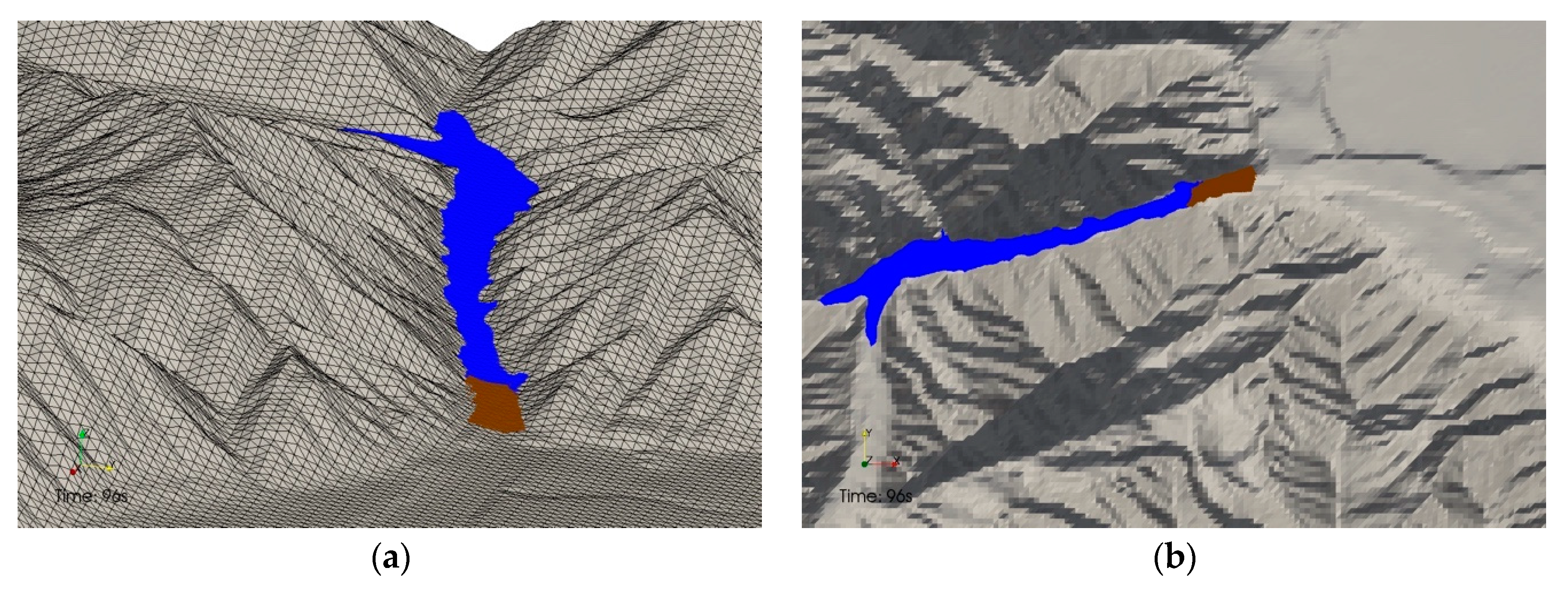
The model above was validated through laboratory experiments [8] and applied to a 3D erosional dam-break flood on complex topography (Figure 6). This demonstrative test case showed the applicability of the SPH method in simulating a flood on complex topography with bed-load transport. The 3D erosional dam break was triggered by an instantaneous and almost complete failure of a gravity dam, whose structure was not simulated. The water flow impacts, thrusts, or erodes, and then transports a portion of the downstream mobile bed, which is composed of a bed of granular material. Its original sedimentation was related to the presence of a weir, whose structure was then removed before the dam building. The 3D fields of the velocity vector and pressure were computed and the 2D fields of the maximum (over time) water depth and specific flow rate (i.e., flow rate per width unit) were elaborated. These quantities, requested for risk analyses, were derived from the particle and the topography heights, and the magnitude of the depth-averaged velocity vectors. The time series of the water depth, the fluid volumes (cumulated in selected sub-domains), and the flow rate were assessed at specific monitoring sections. This demonstrative test, reported in [8] and available as tutorial no. 18 of SPHERA v.9.0.0 [76], shows the potential of the SPH method in simulating a full-scale 3D flood on complex topography with sediment transport. Although validations were reported in terms of comparisons with laboratory datasets [8], these only refer to simplified topographies. A full scale validation still has to be investigated due to the lack of available measures for complex topographies with sediment transport.

CFD codes for flood propagation on complex topography need a suitable numerical chain. A non-exhaustive list of pre-processing and post-processing free tools for floods on complex topography is discussed hereafter.

The dataset SRTM3 (USGS) represents the most accurate open data DEM (“digital elevation model”, not to be confused with the “discrete element method” from Section 2.2) archive with a spatial resolution of 1” (spatial resolution length scale approximately equal to 31 m) and an almost global cover. The SRTM3 files are available in the “.tif” format. The numerical tool GDAL [84] can be used to convert the DEM “.tif” file format of SRTM3 in the alternative format “.dem”. DEM2xyz [85] can read the DEM file (“.dem” format), convert the geographic coordinates in Cartesian coordinates over a regular grid, and write the resulting DEM on an output file (“.xyz” format), possibly coarsening the spatial resolution and reconstructing bathymetry where it is not available. Paraview (Kitware) [86] can read the “.xyz” output file of DEM2xyz and elaborate a 2D Delaunay grid starting from the DEM vertices. Paraview also allows cutting the numerical domain, drawing particular regions of interest (e.g., water bodies), engineering works (e.g., dams), and monitoring elements (e.g., points, lines, surfaces). The above information, derived from Paraview, can be provided to DEM2xyz, which can be executed again to add the new elements designed with Paraview.

The 3D fluid dynamics output files of a CFD code for floods can be further elaborated by means of Grid Interpolator [87], which reads a 3D field of values from an input grid and interpolates them on an output grid with a different spatial resolution. At this point, Paraview can be used to visualize the 2D and 3D fluid dynamics fields and return the associated image files.

All the pre-processing and post-processing items above are FOSS, but SRTM3, which is “open-data” (dataset available upon public and free access) [88] can be used within the same numerical chain and can be replaced by other free or proprietary items depending on the user resources and targets.

4. High Performance Computing Solutions for Complex Hydraulic Engineering Problems

Numerical modeling is becoming more useful and practical thanks to the capability of the current computer hardware. Years ago, significant simplifications of the problem needed to be undertaken in order to make the numerical simulation feasible due to past hardware limitations. Nowadays, thanks to the continuous hardware improvement and the use of HPC techniques that allow for the advantages of the enormous calculation power of the current hardware to be taken, it is possible to now simulate complex problems with fewer simplifications, and problems that were impossible to be simulated due to their spatial and/or temporal scale can now be carried out. Therefore, several codes have been developed that use these HPC techniques to simulate complex hydraulic engineering problems of water-related natural hazards in reasonable execution times. Some examples are SPHERA for sediment transport [8] and landslides [9]; DualSPHysics to model the scouring of two-phase liquid-sediments flows [6,53]; and GPUSPH for simulating lava flows [74]. As explained in [89], due to the limitation of sequential computing and the high cost of increasing performance in sequential architectures, the era of sequential computing was replaced by the era of parallel computing. Currently, hardware performance is fundamentally increased by expanding the number of processing units, instead of increasing the power of a single processing unit. Therefore, it is mandatory to use parallel programming techniques to distribute the workload among the available processing units and synchronize their execution.

OpenMP (Open Multi-Processing) is the most common parallel programming technique for multi-core systems with shared memory because it does not involve major code changes. MPI (message passing interface) is a standard for distributed memory systems that allows for the work to be divided among the multiple calculation nodes connected to each other. On the other hand, and more recently, GPGPU (general-purpose computing on graphics processing units) has emerged as an alternative to the use of traditional CPUs (central processing units). This technique allows the code to be executed on the GPU (graphics processing units). GPUs initially developed for rendering graphics have greatly increased their parallel computing power over the last decade due to the increasing computing demands of the gaming market, and more recently due to the significant growth of markets related to AI (artificial intelligence), DL (deep learning), and DNN (deep neural networks). They are in fact now several times faster than CPUs for problems that demand a high computational cost whilst offering a high degree of parallelism, to which SPH falls under [90]. At the same time, the emergence of programming languages such as CUDA (compute unified device architecture) and OpenCL makes the development of GPU codes easier. These two reasons have encouraged many researchers to implement their models for GPU, thus starting the era of GPU computing [91].

Particle methods such as smoothed particle hydrodynamics (SPH) [92] or moving particle semi-implicit (MPS) [93] have a very high computational cost. The high computational cost of particle methods is due to the fact that each particle has to interact with a large number of neighboring particles, which, in addition, may change every time step. The way that particles are organized in memory and the neighbor search (NS) algorithm is key to maximizing performance in parallel architectures. The most common algorithms for NS are the Verlet list and Cell-linked list. The work in [94] compared both algorithms applied to SPH and, in [95], variants of these algorithms were evaluated to conclude that the Verlet list may be faster than Cell-linked list, but the memory consumption is prohibitive for a high number of particles, so the Cell-linked list was found to be more efficient. The same conclusion was confirmed in [96] for GPU simulations. Quad-tree partitions combined with the Morton space filling curve (SFC) was recommended when using variable resolution in multi-core architectures [97] and GPU devices [98]. The work in [99] proposed another algorithm based on hierarchical cell decomposition for variable resolution in distributed memory architectures using MPI. A very fast NS, where the speed is the main priority, was implemented in [100] for real-time animations, but this approach is invalid for real-physic simulations since some interactions of neighboring particles are missing.

The high computational cost of particle methods can be countered using the programming techniques discussed above. Thus, different implementations of the SPH method using OpenMP can be found [97,101,102], although the same algorithms can be applied to other particle methods. The work of [101] included a performance analysis of SPH in multi-core CPUs and studied how to avoid bottlenecks. The work in [102] implemented an optimized SPH for parallel machines with shared memory and compared the effective computing performance on multi-core CPUs and Xeon Phi MIC (many integrated core) coprocessors with 61 cores. The work in [97] evaluated the efficiency of a neighbor search algorithm based on a quad-tree partitioning on 32 processors. The SPH method has also been implemented for distributed memory systems using MPI for WCSPH [99,103,104,105,106], and MPI for ISPH [107,108]. The execution on distributed systems requires the division of the simulation domain into multiple subdomains. Each subdomain is executed by an independent process, but all processes must be synchronized for every calculation step. Therefore, load balancing between the different processes is essential to minimize the time that each process waits for the rest of the processes with a consequent loss of performance. In addition, this balancing needs to be dynamic where the workload can shift from one subdomain to another during simulation in Lagrangian methods. On the other hand, the decomposition of the domain into distributed memory systems requires the transfer of data between the nodes that process each domain, especially in the case of GPUs where transfers via PCI Express on the node itself are also required. The overhead of these memory transfers can be significant, so it is a major problem in the dynamic decomposition of the domain. In [103], the dynamic load balancing was based on the METIS package. The work in [104] implemented the code JOSEPHINE using the programming language Fortran 90 and OpenMPI, obtaining a good efficiency on 16 processors. The implementation of [99] used a hierarchical cell decomposition to allow variable resolution. The work in [105] obtained a high efficiency with 32,768 CPU cores using a decomposition algorithm based on orthogonal recursive bisection [109]. Most recently, [109] implemented dynamic domain decomposition between Voronoi subdomains and achieved a good speedup using 1024 processes. The work in [107] presented an ISPH solver where a simple spatial domain decomposition in cells was combined with the Hilbert space filling curve (SFC) and load balancing was only applied when particle imbalances were detected. This implementation reported an efficiency of 63%, simulating a still water case with 66.5 million particles on 512 processors compared to the execution time using 32 processors. The ISPH implementation of [108] achieved an efficiency close to 80% on 1536 MPI nodes, simulating a dam break with 100 million particles compared to the runtime using one node with 24 cores. Nowadays, powerful GPUs can be used instead of expensive parallel machines or clusters based on CPU processors to simulate several millions of particles. The first full GPU implementation of the SPH method was reported in [110] using shader programming. Other implementations on GPU are described in the works [52,111,112,113,114,115]. The work in [111] presented the SPH code, named DualSPHysics, implemented for GPU or CPU executions where a Cell-linked list [116] is used for a neighbor search. This work showed a comparison between several GPU models of different generations and several CPU models, achieving an improvement of almost two orders of magnitude. Hérault et al. [112] described another SPH solver for GPU named GPUSPH using a Verlet list. This solver allowed them to simulate lava flows on a complex topography with accuracy and efficiency, obtaining speedups of up to two orders of magnitude with respect to an equivalent CPU as claimed by the authors of [112]. The work in [52] presented an improved DualSPHysics code where the CPU and GPU optimization strategies described in [96] were applied to obtain a fair comparison between GPU and multi-core CPU executions. A multi-phase SPH model for liquid–gas simulations on GPUs based on DualSPHysics was shown in [113]. The use of GPUs is mandatory in this multi-phase approach since both fluids, water, and the surrounding air volume must be discretized in SPH particles. Therefore, the total number of particles and the execution time are usually increased several times. The work in [114] described a 2D SPH code optimized for long hydraulic simulations using the Hilbert space filling curve to improve the data locality and increase the performance. The work in [115] presented the AQUAgpusph code using the programming language OpenCL. The use of OpenCL allows the use of NVIDIA or AMD GPUs and the same code can be executed on multi-core CPUs. GPU implementations of ISPH can be found in [117,118,119]. The work in [117] presented a solver written in OpenCL that could be executed on a CPU or GPU and the performance of both architectures was compared. The work in [118] showed an ISPH code to perform realistic fluid simulations in real time, so some simplifications were applied to increase the speed of execution. The work in [119] implemented an optimized GPU solver starting from [111] and achieved a speedup close to 5 against CPU simulations with 16 threads. GPU implementations of MPS can also be found in [120] for 2D and in [121] for 3D free surface simulations.

Several examples of solvers based on shallow water equations on GPU are in [98,122,123,124,125,126]. These allow for large-scale flood simulations to be performed using only one GPU. The work in [98] presented a SPH solver for shallow water with adaptive resolution using a quad-tree algorithm for neighbor search. The work in [122] presented a 2D flood model that allowed for the simulation of long duration floods in a few minutes. The work in [123] simulated more than one hour of the Malpasset dam failure case in less than 30 s and proved that the use of single precision was enough for that problem. The work in [124] presented a finite volume solver with explicit discretization and an efficient algorithm to deactivate dry zones improving performance. The work in [125] introduced an optimized version of the IBER solver [127] for CPU and GPU simulations. That new version of IBER solved 24 h of an extreme flash flood in less than 10 min. The work in [126] presented a shallow water model based on the finite volume approach implemented for GPU with the OpenACC language [128]. OpenACC allows GPU parallelization to be implemented automatically using compiler directives like OpenMP for CPUs. Some examples of flood simulation, possibly thanks to the computing power of a single GPU, can be found in [18,129,130]. The work in [129] used more than 1.5 million particles to simulate a complicated city layout including underground spaces with the GPUSPH model [112]. The work in [18] simulated runoff on a real terrain generated from photogrammetry information obtained by an UAV (unmanned aerial vehicle). This simulation with 7.5 million particles was performed using the DualSPHysics code [111] and took 138 h for 15 physical minutes. The work in [130] showed a large-scale urban flood performed by the GPU model implemented in [98]. This simulation with 230,000 particles took 135 h to simulate five physical hours.

One GPU can perform simulations with a high particle number in affordable execution times as demonstrated by the works mentioned before. The same results on CPU systems would require expensive CPU clusters. However, a fair comparison between GPU and CPU performance is not straightforward, since optimized solvers for both architectures and hardware from the same period should be used to avoid unreal speedups [116,131]. The work in [132] disproved the speedups of 100x or 1000x as shown in some GPU–CPU comparisons.

Although today’s GPUs provide high computation power, the simulation of real cases implies huge domains with a high resolution, which implies simulating tens or hundreds of million particles and these simulations are not viable in a single GPU due to memory limitations and prohibitive execution times. The solution is to use multi-GPU machines with shared memory or GPU clusters. Examples of multi-GPU SPH solvers can be found in [133,134,135,136]. The work in [133] explored the use of MPI in the DualSPHysics code to perform multi-GPU simulation on GPU clusters. This approach allowed for the simulation of 32 million particles on four GPUs, achieving an efficiency of 80% using weak scaling by simulating eight million particles per GPU. The work in [134] described the implementation of an optimized multi-GPU version of DualSPHysics using an MPI that was able to simulate 1024 million particles on 128 GPUs, achieving almost 100% efficiency using weak scaling by simulating eight million particles per GPU. The work in [135] extended the GPUSPH solver to multi-GPU machines with shared memory using threads and domain decomposition in two dimensions. This implementation is limited by the number of GPUs hosted by one machine or computation node, typically six or eight GPUs. The work in [136] presented a multi-GPU implementation with 3D domain decomposition that achieved 89% efficiency using strong scaling by simulating more than 30 million particles on eight GPUs using MPI.

5. Conclusions and Future Perspectives

This paper collected some recent works showing the application of CFD techniques for modeling problems of practical and theoretical interest involving complex multiphase flows relevant for the analysis and mitigation of water-related natural hazards. The paper focused on meshless techniques for the numerical modeling of fast landslides, tsunami wave, flooding in complex geometry and sediment scouring; few relevant examples have also been mentioned concerning traditional grid-based methods applied to the analysis of environmental risks related to flooding in complex topography. The peculiar features of the examined works in terms of mathematical modeling and numerical implementation have been illustrated and outline the principal differences.

Different approaches are commonly used for modeling the non-Newtonian dynamics of dense granular flows. Some of them consider the sediment as a single-phase moving mass; other approaches model the sediment as a two-phase mixture where the voids of the solid matrix are filled by some liquid phase in order to account for the pore pressure effects. In all of the works examined where the SPH method was applied to the solid, the motion of the granular phase was treated as a pseudo-fluid once the sediment particles had been mobilized. Furthermore, the criterion adopted for determining the onset of sediment motion is, in general, not uniform. In some of the considered works, a numerical threshold was used for this purpose and the involved mechanical parameters, despite their physical meaning, require proper tuning so that the model results can suitably fit the experimental data. This approach is used both in the analysis of bed sediment erosion and landslide run-out where the definition of a triggering threshold that establishes the critical condition for the onset of sediment motion is required. In these cases, the need of tuning parameters, which assume a numerical role rather than a physical meaning, may limit the applicability of the model to those situations of practical interest where calibration data are available. An alternative approach to overcome this limitation is provided by the kinetic theory of dense granular flows (KTGF) that is put into SPH formalism and has been proven to be able to simulate dense granular flows (the so-called “packing limit” of KTGF) and fast landslides with a suitable degree of accuracy.

Proper numerical modeling of the erosion processes that are related to the motion of loose sediment particles suspended in the water flow would require that the size of the numerical particles should be of the same order of the size of real sediment grains; but this task is not allowed in practical problems where the geometrical complexity may induce excessive computational cost. However, reliable results may be obtained by simulating numerical particles as a combination of clear water and turbid water particles that mimic a suspended load.

Concerning the interaction between the phases (i.e., water and sediment), different approaches have been followed. In some cases, the governing equations of motion are solved simultaneously for both phases, thus obtaining coupled dynamics. In other cases, the governing equations are solved separately for each phase and the interface conditions should be enforced to assure kinematic and dynamic continuity between phases through an iterative procedure that can, however, affect the computational time. While some models were examined in terms of the mathematical features, these were not the same methods that were examined in terms of numerical implementation.

The above-mentioned relevant aspects may exert significant influence both in the numerical representation of the multiphase flow and in the reliability of the model results. Therefore, they should be carefully evaluated in the analysis of water-related natural hazards in order to obtain a reliable representation of the investigated problem. Given the complexity (especially geometrical) that usually characterizes the problems of practical interest, these numerical models could be used to support risk analysis and mitigation if appropriate programming techniques and modern architectures for scientific computation are used to obtain fast-running computer codes. This goal is not simple to accomplish, even with the adoption of HPC techniques and parallel computing. The simulation of real cases with large domains and high resolution will probably become more affordable with the use of GPU clusters. However, this task needs better implementation of the identified useful formulations of SPH for multi-GPU multi-node. This requires overcoming the problems associated with domain decomposition and memory transfer across nodes, which are particularly difficult for the fully-coupled two-phase formulations.

References

- Wang, D.; Shao, S.; Li, S.; Shi, Y.; Arikawa, T.; Zhang, H. 3D ISPH erosion model for flow passing a vertical cylinder. J. Fluids Struct. 2018, 78, 374–399. [Google Scholar] [CrossRef]
- Wang, D.; Shaowu, L.; Arikawa, T.; Gen, H. ISPH Simulation of Scour Behind Seawall Due to Continuous Tsunami Overflow. Coast. Eng. J. 2016, 58, 1650014. [Google Scholar] [CrossRef]
- Wang, C.; Peng, C.; Meng, X. Smoothed Particle Hydrodynamics Simulation of Water-Soil Mixture Flows. J. Hydraul. Eng. 2016, 142, 04016032. [Google Scholar] [CrossRef]
- Guandalini, R.; Agate, G.; Manenti, S.; Sibilla, S.; Gallati, M. SPH Based Approach toward the Simulation of Non-cohesive Sediment Removal by an Innovative Technique Using a Controlled Sequence of Underwater Micro-explosions. Procedia IUTAM 2015, 18, 28–39. [Google Scholar] [CrossRef]
- Guandalini, R.; Agate, G.; Manenti, S.; Sibilla, S.; Gallati, M. Innovative numerical modeling to investigate local scouring problems induced by fluvial structures. In Proceedings of the Sixth International Conference on Bridge Maintenance, Safety and Management (IABMAS 2012), Stresa, Italy, 8–12 July 2012; pp. 3110–3116. [Google Scholar]
- Zubeldia, E.H.; Fourtakas, G.; Rogers, B.D.; Farias, M.M. Multi-phase SPH model for simulation of erosion and scouring by means of the shields and Drucker–Prager criteria. Adv. Water Resour. 2018, 117, 98–114. [Google Scholar] [CrossRef]
- Manenti, S.; Sibilla, S.; Gallati, M.; Agate, G.; Guandalini, R. SPH simulation of sediment flushing induced by a rapid water flow. J. Hydraul. Eng. 2012, 138, 272–284. [Google Scholar] [CrossRef]
- Amicarelli, A.; Kocak, B.; Sibilla, S.; Grabe, J. A 3D smoothed particle hydrodynamics model for erosional dam-break floods. Int. J. Comput. Fluid Dyn. 2017, 31, 413–434. [Google Scholar] [CrossRef]
- Manenti, S.; Amicarelli, A.; Todeschini, S. WCSPH with Limiting Viscosity for Modeling Landslide Hazard at the Slopes of Artificial Reservoir. Water 2018, 10, 515. [Google Scholar] [CrossRef]
- Tan, H.; Chen, S. A hybrid DEM-SPH model for deformable landslide and its generated surge waves. Adv. Water Resour. 2017, 108, 256–276. [Google Scholar] [CrossRef]
- Shi, C.; An, Y.; Wu, Q.; Liu, Q.; Cao, Z. Numerical simulation of landslide-generated waves using a soil–water coupling smoothed particle hydrodynamics model. Adv. Water Resour. 2016, 92, 130–141. [Google Scholar] [CrossRef]
- Viroulet, S.; Sauret, A.; Kimmoun, O.; Kharif, C. Granular collapse into water: Toward tsunami landslides. J. Vis. 2013, 16, 189–191. [Google Scholar] [CrossRef]
- Capone, T.; Panizzo, A.; Monaghan, J.J. SPH modeling of water waves generated by submarine landslides. J. Hydraul. Res. 2010, 48, 80–84. [Google Scholar] [CrossRef]
- Bordoni, M.; Meisina, C.; Valentino, R.; Bittelli, M.; Chersich, S. Site-specific to local-scale shallow landslides triggering zones assessment using TRIGRS. Nat. Hazards Earth Syst. Sci. 2015, 15, 1025–1050. [Google Scholar] [CrossRef] [Green Version]
- Zizioli, D.; Meisina, C.; Valentino, R.; Montrasio, L. Comparison between different approaches to modeling shallow landslide susceptibility: A case history in Oltrepo Pavese, Northern Italy. Nat. Hazards Earth Syst. Sci. 2013, 13, 559–573. [Google Scholar] [CrossRef]
- Ray, R.; Deb, K.; Shaw, A. Pseudo-Spring smoothed particle hydrodynamics (SPH) based computational model for slope failure. Eng. Anal. Bound. Elem. 2019, 102, 139–148. [Google Scholar] [CrossRef]
- Gu, S.; Zheng, X.; Ren, L.; Xie, H.; Huang, Y.; Wei, J.; Shao, S. SWE-SPHysics Simulation of Dam Break Flows at South-Gate Gorges Reservoir. Water 2017, 9, 387. [Google Scholar] [CrossRef]
- Barreiro, A.; Domínguez, J.M.; Crespo, A.J.C.; González-Jorge, H.; Roca, D.; Gómez-Gesteira, M. Integration of UAV photogrammetry and SPH modeling of fluids to study runoff on real terrains. PLoS ONE 2014, 9, e111031. [Google Scholar] [CrossRef]
- Vacondio, R.; Mignosa, P.; Pagani, S. 3D SPH numerical simulation of the wave generated by the Vajont rock slide. Adv. Water Res. 2013, 59, 146–156. [Google Scholar] [CrossRef]
- Qiu, L.C.; Liu, Y.; Han, Y. A 3D Simulation of a Moving Solid in Viscous Free-Surface Flows by Coupling SPH and DEM. Math. Probl. Eng. 2017, 2017, 1–7. [Google Scholar] [CrossRef]
- Albano, R.; Sole, A.; Mirauda, D.; Adamowski, J. Modeling large floating bodies in urban area flash-floods via a Smoothed Particle Hydrodynamics model. J. Hydrol. 2016, 541, 344–358. [Google Scholar] [CrossRef]
- Amicarelli, A.; Albano, R.; Mirauda, D.; Agate, G.; Sole, A.; Guandalini, R. A smoothed particle hydrodynamics model for 3D solid body transport in free surface flows. Comput. Fluids 2015, 116, 205–228. [Google Scholar] [CrossRef]
- Lu, N.; Godt, J. Hillslope Hydrology and Stability; Cambridge University Press: New York, NY, USA, 2013. [Google Scholar]
- Iverson, R.M. Landslide triggering by rain infiltration. Water Resour. Res. 2000, 36, 1897–1910. [Google Scholar] [CrossRef] [Green Version]
- Iverson, R.M. The physics of debris flows. Rev. Geophys. 1997, 35, 245–296. [Google Scholar] [CrossRef] [Green Version]
- Inam, A.; Adamowski, J.; Prasher, S.; Halbe, J.; Malard, J.; Albano, R. Coupling of a distributed stakeholder-built system dynamics socio-economic model with SAHYSMOD for sustainable soil salinity management—Part 1: Model development. J. Hydrol. 2017, 55, 596–618. [Google Scholar] [CrossRef]
- Shao, S. Incompressible smoothed particle hydrodynamics simulation of multi-fluid flows. Int. J. Numer. Meth. Fluids 2012, 69, 1715–1735. [Google Scholar] [CrossRef]
- Manenti, S. Standard WCSPH for free-surface multi-phase flows with a large density ratio. Int. J. Ocean Coast. Eng. 2018, 1. [Google Scholar] [CrossRef]
- Colagrossi, A.; Landrini, M. Numerical simulation of interfacial ows by smoothed particle hydrodynamics. J. Comput. Phys. 2003, 191, 448–475. [Google Scholar] [CrossRef]
- Hu, X.Y.; Adams, N.A. An incompressible multi-phase SPH method. J. Comput. Phys. 2007, 227, 264–278. [Google Scholar] [CrossRef]
- Grenier, N.; Antuono, M.; Colagrossi, A.; le Touzé, D.; Alessandrini, B. An Hamiltonian interface SPH formulation for multi-fluid and free-surface flows. J. Comput. Phys. 2009, 228, 380–393. [Google Scholar] [CrossRef]
- Monaghan, J.J.; Ashkan, R. A simple SPH algorithm for multi-fluid ow with high density ratios. Int. J. Numer. Methods Fluids 2013, 71, 537–561. [Google Scholar] [CrossRef]
- Bouscasse, B.; Colagrossi, A.; Marrone, S.; Souto-Iglesias, A. SPH modelling of viscous flow past a circular cylinder interacting with a free surface. Comput. Fluids 2017, 146, 190–212. [Google Scholar] [CrossRef]
- Hamill, L. Bridge Hydraulics; E&FN Spon: New York, NY, USA, 1999. [Google Scholar]
- Persi, E.; Petaccia, G.; Fenocchi, A.; Manenti, S.; Ghilardi, P.; Sibilla, S. Hydrodynamic coefficients of yawed cylinders in open-channel flow. Flow Meas. Instrum. 2019, 65, 288–296. [Google Scholar] [CrossRef]
- Dordoni, S.; Malerba, P.; Sgambi, L.; Manenti, S. Fuzzy reliability assessment of bridge piers in presence of scouring. In Proceedings of the 5th International Conference on Bridge Maintenance, Safety and Management, Philadelphia, PA, USA, 11–15 July 2010; pp. 1388–1395. [Google Scholar]
- Sumer, B.M.; Fredsøe, J. The Mechanics of Scour in the Marine Environment; Advanced Series on Ocean Engineering; World Scientific Publishing Company: Singapore, 2002; Volume 17. [Google Scholar]
- Whitehouse, R.J.S. Scour at Marine Structures; Thomas Telford: London, UK, 1998. [Google Scholar]
- Wang, D.; Arikawa, T.; Li, S.W.; Gen, H. Numerical Simulation on Scour behind Seawall due to Tsunami Overflow. In Proceedings of the Coastal Structures & Solutions to Coastal Disasters Joint Conference, Boston, MA, USA, 9–11 September 2015; ASCE: Reston, VA, USA, 2015. [Google Scholar]
- Li, S.W.; Wang, D. Tsunami occurrences in China and numerical simulation of a supposed tsunami process in Bohai Sea. In Proceedings of the China Ocean Engineering, Dailian, China, August 2013; pp. 490–496. Available online: http://cpfd.cnki.com.cn/Article/CPFDTOTAL-HYGC201308001076.htm (accessed on 30 August 2013).
- Sugano, T.; Nozu, A.; Kohama, E.; Shimosako, K.; Kikuchi, Y. Damage to coastal structures. Soils Found. 2014, 54, 883–901. [Google Scholar] [CrossRef] [Green Version]
- Takahashi, H.; Sassa, S.; Morikawa, Y.; Takano, D.; Maruyama, K. Stability of caisson-type breakwater foundation under tsunami-induced seepage. Soils Found. 2014, 54, 789–805. [Google Scholar] [CrossRef] [Green Version]
- Nakamura, T.; Mizutani, N. Sediment Transport Calculation Considering Laminar and Turbulent Resistance Forces Caused by Infiltration/Exfiltration and its Application to Tsunami-induced Local Scouring. J. Offshore Mech. Arct. Eng. 2013, 136, 011105. [Google Scholar] [CrossRef]
- Oie, T.; Dong, W.; Takatani, T.; Araki, K.; Shaowu, L.; Goto, H.; Arikawa, T. Numerical simulation of scouring behind the seawall caused by tsunami overflow with accurate ISPH method. Jpn. Soc. Civ. Eng. 2015, 71, 253–258. (In Japanese) [Google Scholar]
- Ettema, R.; Kirkil, G.; Muste, M. Similitude of large-scale turbulence in experiments on local scour at cylinders. J. Hydraul. Eng. 2006, 132, 33–40. [Google Scholar] [CrossRef]
- Sun, P.N.; Colagrossi, A.; Marrone, S.; Antuono, M.; Zhang, A.M. Multi-resolution Delta-plus-SPH with tensile instability control: Towards high Reynolds number flows. Comput. Phys. Commun. 2018, 224, 63–80. [Google Scholar] [CrossRef]
- Zhang, A.; Sun, P.; Ming, F. An SPH modeling of bubble rising and coalescing in three dimensions. Comput. Methods Appl. Mech. Eng. 2015, 294, 189–209. [Google Scholar] [CrossRef]
- Ming, F.R.; Sun, P.N.; Zhang, A.M. Numerical investigation of rising bubbles bursting at a free surface through a multiphase SPH model. Meccanica 2017, 52, 2665–2684. [Google Scholar] [CrossRef]
- Ran, Q.; Tong, J.; Shao, S.; Fu, X.; Xu, Y. Incompressible SPH scour model for movable bed dam break flows. Adv. Water Resour. 2015, 82, 39–50. [Google Scholar] [CrossRef] [Green Version]
- Gotoh, H.; Ikari, H.; Memita, T.; Sakai, T. Lagrangian Particle Method for Simulation of Wave Overtopping on a Vertical Seawall. Coast. Eng. J. 2005, 47, 157–181. [Google Scholar] [CrossRef]
- Ulrich, C.; Leonardi, M.; Rung, T. Multi-physics SPH simulation of complex marine-engineering hydrodynamic problems. Ocean Eng. 2013, 64, 109–121. [Google Scholar] [CrossRef]
- Crespo, A.J.C.; Domínguez, J.M.; Rogers, B.D.; Gómez-Gesteira, M.; Longshaw, S.; Canelas, R.; Vacondio, R.; Barreiro, A.; García-Feal, O. DualSPHysics: Open-source parallel CFD solver based on smoothed particle hydrodynamics (SPH). Comput. Phys. Commun. 2015, 187, 204–216. [Google Scholar] [CrossRef]
- Fourtakas, G.; Rogers, B.D. Modeling multi-phase liquid-sediment scour and resuspension induced by rapid flows using Smoothed Particle Hydrodynamics (SPH) accelerated with a Graphics Processing Unit (GPU). Adv. Water Resour. 2016, 92, 186–199. [Google Scholar] [CrossRef]
- Vand, V. Viscosity of solutions and suspensions. I. Theory. J. Phys. Colloid Chem. 1948, 52, 277–299. [Google Scholar] [CrossRef] [PubMed]
- Todeschini, S. Trends in long daily rainfall series of Lombardia (Northern Italy) affecting urban stormwater control. Int. J. Climatol. 2012, 32, 900–919. [Google Scholar] [CrossRef]
- Todeschini, S.; Papiri, S.; Ciaponi, C. Placement Strategies and Cumulative Effects of Wet-weather Control Practices for Intermunicipal Sewerage Systems. Water Resour. Manag. 2018, 32, 2885–2900. [Google Scholar] [CrossRef]
- Stancanelli, L.M.; Peres, D.J.; Cancelliere, A.; Foti, E. A combined triggering-propagation modeling approach for the assessment of rainfall induced debris flow susceptibility. J. Hydrol. 2017, 550, 130–143. [Google Scholar] [CrossRef] [Green Version]
- Baum, R.L.; Savage, W.Z.; Godt, J.W. TRIGRS—A FORTRAN Program for Transient Rainfall Infiltration and Grid-Based Regional Slope-Stability Analysis, Version 2.0; U.S. Geological Survey: Reston, VA, USA, 2008.
- O’Brien, J. Flo-2d User’s Manual, version 2006.01; flo-2d Software. Inc.: Nutrioso, AZ, USA, 2006. [Google Scholar]
- Dai, F.C.; Lee, C.F.; Ngai, Y.Y. Landslide risk assessment and management: An overview. Eng. Geol. 2002, 64, 65–87. [Google Scholar] [CrossRef]
- Pastor, M.; Haddad, B.; Sorbino, G.; Cuomo, S.; Drempetic, V. A depth-integrated, coupled SPH model for flow-like landslides and related phenomena. Int. J. Numer. Anal. Methods Geomech. 2009, 33, 143–172. [Google Scholar] [CrossRef]
- Pastor, M.; Quecedo, M.; González, E.; Herreros, I.; Merodo, J.A.F.; Mira, P. A simple approximation to bottom friction for Bingham fluid depth integrated models. J. Hydraul. Eng. 2004, 130, 149–155. [Google Scholar] [CrossRef]
- Rendina, I.; Viccione, G.; Cascini, L. Kinematics of flow mass movements on inclined surfaces. Theor. Comput. Fluid Dyn. 2019, 33, 107–123. [Google Scholar] [CrossRef]
- Shao, S.; Lo, E.Y.M. Incompressible SPH method for simulating Newtonian and non-Newtonian flows with a free surface. Adv. Water Resour. 2003, 26, 787–800. [Google Scholar] [CrossRef]
- Albano, R.; Craciun, I.; Mancusi, L.; Sole, A.; Ozunu, A. Flood damage assessment and uncertainity analysis: the case study of 2006 flood in Ilisua Basin in Romania. Carpath. J. Earth. Environ. Sci. 2017, 2, 12. [Google Scholar]
- Di Risio, M.; Bellotti, G.; Panizzo, A.; de Girolamo, P. Three-dimensional experiments on landslide generated waves at a sloping coast. Coast. Eng. 2009, 56, 659–671. [Google Scholar] [CrossRef]
- Panizzo, A.; de Girolamo, P.; di Risio, M.; Maistri, A.; Petaccia, A. Great landslide events in Italian artificial reservoirs. Nat. Hazards Earth Syst. Sci. 2005, 5, 733–740. [Google Scholar] [CrossRef] [Green Version]
- Fritz, H.M.; Hager, W.H.; Minor, H.E. Lituya Bay case: Rockslide impact and wave run-up. Sci. Tsunami Hazards 2001, 19, 3–22. [Google Scholar]
- Marrone, S.; Antuono, M.; Colagrossi, A.; Colicchio, G.; le Touzé, D.; Graziani, G. δ-SPH model for simulating violent impact flows. Comput. Methods Appl. Mech. Eng. 2011, 200, 1526–1542. [Google Scholar] [CrossRef]
- Heinrich, P. Nonlinear water waves generated by submarine and aerial landslides. J. Waterw. Port Coast. Ocean Eng. 1992, 118, 249–266. [Google Scholar] [CrossRef]
- Xu, W.J.; Dong, X.Y.; Ding, W.T. Analysis of fluid-particle interaction in granular materials using coupled SPH-DEM method. Powder Technol. 2019, 353, 459–472. [Google Scholar] [CrossRef]
- Canelas, R.B.; Dominiguez, J.M.; Crespo, A.J.C.; Gomez-Gesteira, M.; Ferreira, R.M.L. Resolved Simulation of a granular-fluid flow with a coupled SPH-DCDEM model. J. Hydraul. Eng. 2017, 143, 6017012. [Google Scholar] [CrossRef]
- Zago, V.; Bilotta, G.; Hérault, A.; Dalrymple, R.A.; Fortuna, L.; Cappello, A.; Ganci, G.; del Negro, C. Semi-implicit 3D SPH on GPU for lava flows. J. Comp. Phys. 2018, 375, 854–870. [Google Scholar] [CrossRef]
- Manenti, S.; Pierobon, E.; Gallati, M.; Sibilla, S.; D’Alpaos, L.; Macchi, E.; Todeschini, S. Vajont Disaster: Smoothed Particle Hydrodynamics Modeling of the Postevent 2D Experiments. J. Hydraul. Eng. 2016, 142, 5015007. [Google Scholar] [CrossRef]
- Amicarelli, A.; Manenti, S.; Albano, R.; Agate, G.; Paggi, M.; Longoni, L.; Mirauda, D.; Ziane, L.; Viccione, G.; Todeschini, S.; et al. SPHERA v.9.0.0: A Computational Fluid Dynamics research code, based on the Smoothed Particle Hydrodynamics mesh-less method. Comput. Phys. Commun. 2019. submitted. [Google Scholar]
- SPHERA v.9.0.0 (RSE SpA). Available online: https://github.com/AndreaAmicarelliRSE/SPHERA (accessed on 21 February 2019).
- Aristodemo, F.; Merignolo, D.D.; Groenenboom, P.; Schiavo, A.L.; Veltri, P.; Veltri, M. Assessment of Dynamic Pressures at Vertical and Perforated Breakwaters through Diffusive SPH Schemes. Math. Probl. Eng. 2015, 2015, 1–10. [Google Scholar] [CrossRef]
- Chauchat, J.; Médale, M. A three-dimensional numerical model for incompressible two-phase flow of a granular bed submitted to a laminar shearing flow. Comput. Methods Appl. Mech. Eng. 2010, 199, 439–449. [Google Scholar] [CrossRef] [Green Version]
- Fraccarollo, L.; Capart, H.; Zech, Y. A Godunov method for the computation of erosional shallow water transients. Int. J. Numer. Meth. Fluids 2003, 41, 951–976. [Google Scholar] [CrossRef]
- Soares-Frazão, S.; Zech, Y. Experimental study of dam-break flow against an isolated obstacle. J. Hydraul. Res. 2007, 45 (Suppl. 1), 27–36. [Google Scholar] [CrossRef]
- Lin, P.; Wu, Y.; Bai, J.; Lin, Q. A numerical study of dam-break flow and sediment transport from a quake lake. J. Earthq. Tsunami 2011, 5, 401–428. [Google Scholar] [CrossRef]
- Wu, W.; Jiang, E.; China, P.R.; Wang, S.S. Depth-averaged 2-D calculation of flow and sediment transport in the lower Yellow River. Int. J. River Basin Manag. 2004, 2, 51–59. [Google Scholar] [CrossRef]
- Armstrong, L.; Gu, S.; Luo, K. Study of wall-to-bed heat transfer in a bubbling fluidised bed using the kinetic theory of granular flow. Int. J. Heat Mass Transf. 2010, 53, 4949–4959. [Google Scholar] [CrossRef]
- GDAL (OSGEO). Available online: https://github.com/OSGeo/gdal (accessed on 16 April 2019).
- DEM2xyz (RSE SpA). Available online: https://github.com/AndreaAmicarelliRSE/DEM2xyz (accessed on 16 April 2019).
- Paraview (Kitware). Available online: https://github.com/Kitware/ParaView (accessed on 16 April 2019).
- Grid Interpolator (RSE SpA). Available online: https://github.com/AndreaAmicarelliRSE/Grid_Interpolator (accessed on 16 April 2019).
- SRTM3/DTED1 (USGS). Available online: http://earthexplorer.usgs.gov/ (accessed on 16 April 2019).
- Baker, M.; Buyya, R. Cluster Computing at a Glance. In High Performance Cluster Computing—Architectures and Systems; Prentice Hall PTR: Upper Saddle River, NJ, USA, 1999; pp. 3–47. [Google Scholar]
- Nickolls, J.; Buck, I.; Garland, M.; Skadron, K. Scalable Parallel Programming with CUDA. Queue GPU Comput. 2008, 6, 40–53. [Google Scholar] [CrossRef] [Green Version]
- Nickolls, J.; Dally, W.J. The GPU computing era. IEEE Micro 2010, 30, 56–69. [Google Scholar] [CrossRef]
- Monaghan, J.J. Smoothed particle hydrodynamics. Ann. Rev. Astronom. Astrophys. 1992, 30, 543–574. [Google Scholar] [CrossRef]
- Koshizuka, S.; Oka, Y. Moving Particle Semi-Implicit Method for Fragmentation of Incompressible Fluid. Nucl. Sci. Eng. 1996, 123, 421–434. [Google Scholar] [CrossRef]
- Viccione, G.; Bovolin, V.; Carratelli, E.P. Defining and optimizing algorithms for neighbouring particle identification in SPH fluid simulations. Int. J. Numer. Methods Fluids 2008, 58, 625–638. [Google Scholar] [CrossRef]
- Domínguez, J.M.; Crespo, A.J.C.; Gómez-Gesteira, M.; Marongiu, J.C. Neighbour lists in smoothed particle hydrodynamics. Int. J. Numer. Methods Fluids 2011, 67, 2026–2042. [Google Scholar] [CrossRef]
- Winkler, D.; Rezavand, M.; Rauch, W. Neighbour lists for smoothed particle hydrodynamics on GPUs. Comput. Phys. Commun. 2018, 225, 140–148. [Google Scholar] [CrossRef]
- Wang, D.; Zhou, Y.; Shao, S. Efficient Implementation of Smoothed Particle Hydrodynamics (SPH) with Plane Sweep Algorithm. Commun. Comput. Phys. 2016, 19, 770–800. [Google Scholar] [CrossRef]
- Xia, X.; Liang, Q. A GPU-accelerated smoothed particle hydrodynamics (SPH) model for the shallow water equations. Environ. Model. Softw. 2016, 75, 28–43. [Google Scholar] [CrossRef]
- Gonnet, P. Efficient and Scalable Algorithms for Smoothed Particle Hydrodynamics on Hybrid Shared/Distributed-Memory Architectures. SIAM J. Sci. Comput. 2014, 37, C95–C121. [Google Scholar] [CrossRef]
- Joselli, M.; Junior, J.R.d.; Clua, E.W.; Montenegro, A.; Lage, M.; Pagliosa, P. Neighborhood grid: A novel data structure for fluids animation with GPU computing. J. Parallel Distrib. Comput. 2015, 75, 20–28. [Google Scholar] [CrossRef]
- Wenbo, C.; Yao, Y.; Zhang, Y. Performance analysis of parallel smoothed particle hydrodynamics on multi-core CPUs. In Proceedings of the 2014 International Conference on Cloud Computing and Internet of Things, Changchun, China, 13–14 December 201.
- Nishiura, D.; Furuichi, M.; Sakaguchi, H. Computational performance of a smoothed particle hydrodynamics simulation for shared-memory parallel computing. Comput. Phys. Commun. 2015, 194, 18–32. [Google Scholar] [CrossRef]
- Ferrari, A.; Dumbser, M.; Toro, E.F.; Armanini, A. A new 3D parallel SPH scheme for free surface flows. Comput. Fluids 2009, 38, 1203–1217. [Google Scholar] [CrossRef]
- Cherfils, J.M.; Pinon, G.; Rivoalen, E. JOSEPHINE: A parallel SPH code for free-surface flows. Comput. Phys. Commun. 2012, 183, 1468–1480. [Google Scholar] [CrossRef]
- Oger, G.; Le Touzé, D.; Guibert, D.; De Leffe, M.; Biddiscombe, J.; Soumagne, J.; Piccinali, J.-G. On distributed memory MPI-based parallelization of SPH codes in massive HPC context. Comput. Phys. Commun. 2016, 200, 1–14. [Google Scholar] [CrossRef]
- Egorova, M.S.; Dyachkov, S.A.; Parshikov, A.N.; Zhakhovsky, V.V. Parallel SPH modeling using dynamic domain decomposition and load balancing displacement of Voronoi subdomains. Comput. Phys. Commun. 2019, 234, 112–125. [Google Scholar] [CrossRef]
- Yeylaghi, S.; Moa, B.; Oshkai, P.; Buckham, B.; Crawford, C. ISPH modeling for hydrodynamic applications using a new MPI-based parallel approach. J. Ocean Eng. Mar. Energy 2017, 3, 35–50. [Google Scholar] [CrossRef]
- Guo, X.; Rogers, B.D.; Lind, S.; Stansby, P.K. New massively parallel scheme for Incompressible Smoothed Particle Hydrodynamics (ISPH) for highly nonlinear and distorted flow. Comput. Phys. Commun. 2018, 233, 16–28. [Google Scholar] [CrossRef]
- Fleissner, F.; Eberhard, P. Parallel load-balanced simulation for short-range interaction particle methods with hierarchical particle grouping based on orthogonal recursive bisection. Int. J. Numer. Methods Eng. 2008, 74, 531–553. [Google Scholar] [CrossRef]
- Harada, T.; Koshizuka, S.; Kawaguchi, Y. Smoothed particle hydrodynamics on GPUs. In Proceedings of the Computer Graphics International Conference, Petròpolis, Brazil, 30 March 2007; pp. 63–70. Available online: https://pdfs.semanticscholar.org/a132/6b93316e7ce4d2580bd5e3928ce6ff24e386.pdf (accessed on 21 February 2019).
- Crespo, A.C.; Dominguez, J.M.; Barreiro, A.; Gómez-Gesteira, M.; Rogers, B.D. GPUs, a new tool of acceleration in CFD: Efficiency and reliability on smoothed particle hydrodynamics methods. PLoS ONE 2011, 6, e20685. [Google Scholar] [CrossRef] [PubMed]
- Hérault, A.; Bilotta, G.; Vicari, A.; Rustico, E.; del Negro, C. Numerical simulation of lava flow using a GPU SPH model. Ann. Geophys. 2011, 54. [Google Scholar] [CrossRef]
- Mokos, A.; Rogers, B.D.; Stansby, P.K.; Domínguez, J.M. Multi-phase SPH modeling of violent hydrodynamics on GPUs. Comput. Phys. Commun. 2015, 196, 304–316. [Google Scholar] [CrossRef]
- Winkler, D.; Meister, M.; Rezavand, M.; Rauch, W. gpuSPHASE—A shared memory caching implementation for 2D SPH using CUDA. Comput. Phys. Commun. 2017, 213, 165–180. [Google Scholar] [CrossRef]
- Cercos-Pita, J.L. AQUAgpusph, a new free 3D SPH solver accelerated with OpenCL. Comput. Phys. Commun. 2015, 192, 295–312. [Google Scholar] [CrossRef]
- Domínguez, J.M.; Crespo, A.J.C.; Gómez-Gesteira, M. Optimization strategies for CPU and GPU implementations of a smoothed particle hydrodynamics method. Comput. Phys. Commun. 2013, 184, 617–627. [Google Scholar] [CrossRef]
- Qiu, L.C. OpenCL-Based GPU Acceleration of ISPH Simulation for Incompressible Flows. Appl. Mech. Mater. 2014, 444, 380–384. [Google Scholar] [CrossRef]
- Nie, X.; Chen, L.; Xiang, T. Real-Time Incompressible Fluid Simulation on the GPU. Int. J. Comput. Games Technol. 2015, 2015, 417417. [Google Scholar] [CrossRef]
- Chow, A.D.; Rogers, B.D.; Lind, S.J.; Stansby, P.K. Incompressible SPH (ISPH) with fast Poisson solver on a GPU. Comput. Phys. Commun. 2018, 226, 81–103. [Google Scholar] [CrossRef]
- Hori, C.; Gotoh, H.; Ikari, H.; Khayyer, A. GPU-acceleration for Moving Particle Semi-Implicit method. Comput. Fluids 2011, 51, 174–183. [Google Scholar] [CrossRef] [Green Version]
- Kakuda, K.; Nagashima, T.; Hayashi, Y.; Obara, S.; Toyotani, J.; Miura, S. Three-dimensional fluid flow simulations using GPU-based particle method. Comput. Model. Eng. Sci. 2013, 95, 363–376. [Google Scholar]
- Kalyanapu, A.J.; Shankar, S.; Pardyjak, E.R.; Judi, D.R.; Burian, S.J. Assessment of GPU computational enhancement to a 2D flood model. Environ. Model. Softw. 2011, 26, 1009–1016. [Google Scholar] [CrossRef]
- Brodtkorb, A.R.; Sætra, M.L.; Altinakar, M. Efficient shallow water simulations on GPUs: Implementation, visualization, verification, and validation. Comput. Fluids 2012, 55, 1–12. [Google Scholar] [CrossRef]
- Vacondio, R.; Palù, A.D.; Mignosa, P. GPU-enhanced finite volume shallow water solver for fast flood simulations. Environ. Model. Softw. 2014, 57, 60–75. [Google Scholar] [CrossRef]
- García-Feal, O.; González-Cao, J.; Gómez-Gesteira, M.; Cea, L.; Domínguez, J.M.; Formella, A. An accelerated tool for flood modeling based on Iber. Water 2018, 10, 1459. [Google Scholar] [CrossRef]
- Liu, Q.; Qin, Y.; Li, G. Fast simulation of large-scale floods based on GPU parallel computing. Water 2018, 10, 589. [Google Scholar] [CrossRef]
- Bladé, E.; Cea, L.; Corestein, G.; Escolano, E.; Puertas, J.; Vázquez-Cendón, E.; Dolz, J.; Coll, A. Iber: Herramienta de simulación numérica del flujo en ríos. Rev. Int. Metod. Numer. Calc. Disen. Ing. 2014, 30, 1–10. [Google Scholar] [CrossRef]
- Wolfe, M.; Lee, S.; Kim, J.; Tian, X.; Xu, R.; Chapman, B.; Chandrasekaran, S. The OpenACC data model: Preliminary study on its major challenges and implementations. Parallel Comput. 2018, 78, 15–27. [Google Scholar] [CrossRef]
- Hérault, A.; Zhang, H.; Dalrymple, R.A.; Yang, R.; Wu, J. Numerical modeling of dam-break flood through intricate city layouts including underground spaces using GPU-based SPH method. J. Hydrodyn. 2014, 25, 818–828. [Google Scholar]
- Liang, Q.; Xia, X.; Hou, J. Efficient urban flood simulation using a GPU-accelerated SPH model. Environ. Earth Sci. 2015, 74, 7285–7294. [Google Scholar] [CrossRef]
- Dickson, N.G.; Karimi, K.; Hamze, F. Importance of explicit vectorization for CPU and GPU software performance. J. Comput. Phys. 2011, 230, 5383–5398. [Google Scholar] [CrossRef] [Green Version]
- Lee, V.W.; Kim, C.; Chhugani, J.; Deisher, M. Debunking the 100X GPU vs. CPU Myth: An Evaluation of Throughput Computing on CPU and GPU. ACM SIGARCH Comput. Arch. News 2010, 38, 451–460. [Google Scholar] [CrossRef]
- Valdez-Balderas, D.; Domínguez, J.M.; Rogers, B.D.; Crespo, A.J.C. Towards accelerating smoothed particle hydrodynamics simulations for free-surface flows on multi-GPU clusters. J. Parallel Distrib. Comput. 2013, 73, 1483–1493. [Google Scholar] [CrossRef]
- Domínguez, J.M.; Crespo, A.J.C.; Valdez-Balderas, D.; Rogers, B.D.; Gómez-Gesteira, M. New multi-GPU implementation for smoothed particle hydrodynamics on heterogeneous clusters. Comput. Phys. Commun. 2013, 184, 1848–1860. [Google Scholar] [CrossRef]
- Rustico, E.; Bilotta, G.; Herault, A.; del Negro, C.; Gallo, G. Advances in multi-GPU smoothed particle hydrodynamics simulations. IEEE Trans. Parallel Distrib. Syst. 2014, 25, 43–52. [Google Scholar] [CrossRef]
- Ji, Z.; Xu, F.; Takahashi, A.; Sun, Y. Large scale water entry simulation with smoothed particle hydrodynamics on single- and multi-GPU systems. Comput. Phys. Commun. 2016, 209, 1–12. [Google Scholar] [CrossRef]
Figure 1.
Rheological models for non-cohesive sediment erosion with bed load transport and for dense granular flows. I2: second invariant of the rate of deformation tensor; μapp: apparent viscosity.
Figure 2.
Snapshots of incompressible smoothed particle hydrodynamics (ISPH) calculated equilibrium scouring pit with different overflow depth: (a) η = 3.3 cm; (b) η = 4.7 cm, and (c) η = 6.0 cm.
Figure 3.
ISPH computed sediment bed scouring process: (a) snapshots of ISPH calculated vorticity in the scouring pit; (b) Snapshots of the ISPH calculated scouring pit.
Figure 4.
Frames of the 2D smoothed particle hydrodynamics (SPH) simulation of the rainfall induced shallow landslide occurred on April 2009 at Recoaro, Oltrepò Pavese (Northern Italy). (a) Velocity field; (b) Density field.
Figure 5.
Frames of the simulation of the Padua experiment. (a) Velocity field; (b) Density field.
Figure 6.
Demonstrative test case for the meshless SPH method applied to a 3D erosional dam-break flood on complex topography [8]. (a) 3D view. (b) Top view. Digital elevation model (grey, with a black vertex triangulation), liquid SPH particles (blue), mixture SPH particles (brown).
© 2019 by the authors. Licensee MDPI, Basel, Switzerland. This article is an open access article distributed under the terms and conditions of the Creative Commons Attribution (CC BY) license (http://creativecommons.org/licenses/by/4.0/).
Share and Cite
MDPI and ACS Style
Manenti, S.; Wang, D.; Domínguez, J.M.; Li, S.; Amicarelli, A.; Albano, R. SPH Modeling of Water-Related Natural Hazards. Water 2019, 11, 1875. https://doi.org/10.3390/w11091875
AMA Style
Manenti S, Wang D, Domínguez JM, Li S, Amicarelli A, Albano R. SPH Modeling of Water-Related Natural Hazards. Water. 2019; 11(9):1875. https://doi.org/10.3390/w11091875
Chicago/Turabian StyleManenti, Sauro, Dong Wang, José M. Domínguez, Shaowu Li, Andrea Amicarelli, and Raffaele Albano. 2019. "SPH Modeling of Water-Related Natural Hazards" Water 11, no. 9: 1875. https://doi.org/10.3390/w11091875
Note that from the first issue of 2016, this journal uses article numbers instead of page numbers. See further details here.