Estimating Peak Daily Water Demand under Different Climate Change and Vacation Scenarios


KWR Water Research Institute, Groningenhaven 7, 3433 PE Nieuwegein, The Netherlands
*
Author to whom correspondence should be addressed.
Water 2019, 11(9), 1874; https://doi.org/10.3390/w11091874
Submission received: 4 July 2019
/
Revised: 29 August 2019
/
Accepted: 4 September 2019
/
Published: 9 September 2019
(This article belongs to the Section Water Use and Scarcity)
Abstract
:Extremes in drinking water demand are commonly quantified with a so called peaking factor, a probabilistic ratio expressing the daily water demand relative to its annual average corresponding with a once in ten year recurrence period. In this study, we present a modeling framework that allows one to quantify of the impact of climate change and variations in vacation absence on the peaking factor for specific geographic regions. The framework consists of a support vector regression model that simulates daily water demand as a function of meteorological parameters and vacation absence, coupled to an extreme value model that translates simulation results to a peaking factor. After initial model development, we simulated the effects of different climate change/vacation scenarios for 2050 on eight water supply areas in the Netherlands and Belgium. We found that on average there is a net increase in water demand of 0.8% in 2050 and a 6.5% increase in peak demand compared to the reference period.
1. Introduction
Drinking water utilities rely on robust long-term drinking water demand forecasts for adequate planning of production and storage capacity. Two key metrics for these purposes are prediction of (a) the average daily drinking water demand and (b) the extremes in daily drinking water demand [1]. For the first metric, a common practice among water utilities is to develop long term (monthly, yearly) projections based on the analysis and extrapolation of autonomous trends that may influence drinking water demand in the future [2]. Examples of such trends are: Demographic changes, economic development [3,4] and in some cases climate change [4,5]. A characteristic trait of these trends is that they generally develop slowly over the course of years. Their effect on water demand is therefore generally expressed as an annual growth rate.
Extremes in water demand typically unfold on a short timescale (days) and are stochastic in nature. They are therefore usually quantified with a so called peaking factor, a single probabilistic ratio expressing the peak daily water demand corresponding with a once in N year recurrence period (in the Netherlands and Belgium a once in 10 years period is used). Typically, investments in drinking water infrastructure are based on this factor (which is then multiplied by the average demand, which might in itself also increase or decrease in the future).
Given the long lifespan of infrastructure, failure to accurately estimate the peaking factor in the design phase of new infrastructure can lead to under- or over-estimation of capacity requirements. In practice, the peaking factor is often calculated directly from historical water demand time series, thereby not explicitly including any changes in the demand regime that may occur in the nearby future, such as climate change or evolving socio-economical dynamics. Our hypothesis is that this practice may lead to significant over- or under-estimation of future capacity requirements and therefore unforeseen costs. We argue that it would be better to not calculate the daily peaking factor directly from historical time series, but instead from forecasted water demand time series that are representative for the future period.
Most scientific research on water demand forecasting is focused on either the short-term (essentially predicting the water demand for the upcoming days in order to optimize operational control) or long-term (estimating water demand for the years to come). Whereas short-term forecasting is typically done on daily, hourly or even quarterly time steps, long-term forecasting usually leads to results with monthly or yearly simulation time steps [2,6,7]. For the use case that we have in mind, we essentially need a combination of both approaches: We want to simulate water demand characteristics on a daily time step, but for future periods with a length of decades. Our goal is not to predict the exact water demand on a certain day many years ahead in the future, but rather to simulate water demand time series that are statistically representative for the future period using a probabilistic approach. The simulated time series can then be used to calculate the frequency of occurrence of extreme water demands.
As the peaking factor solely expresses the likelihood of water demand peaks within a year, it is not necessary to include all possible influencing trends in our analysis. Any trend that slowly influences water demand over the course of multiple years does not influence the peaking factor. For example, gradual population growth and economic growth generally increases the cumulative water demand in a region over the course of years. However, the intra-annual fluctuations in demand (relative to the annual mean) are not necessarily affected by such a trend. We therefore focus only on trends that have the potential to influence future intra-annual demand fluctuations: Climate change and changes in vacation absence/presence (tourism). The idea here is that by including these trends, we can arrive at a robust estimate for the peaking factor that water utilities can combine with their regular year-to-year forecasts of average water demand growth.
Although in this context climate change in itself can be considered a gradual process, resulting weather is broadly recognized as an important exogenous factor influencing daily drinking water demand [8,9,10]. Therefore daily weather predictions are generally used as input for short-term water demand forecasting (essentially predicting the water demand for the upcoming days in order to optimize operational control). For example, Bakker and Van Duist [8] show that change in temperature influences short-term forecast errors. In a study for the city Melbourne, Zhou and McMahon [11] show how seasonal variation in water demand can be attributed to air temperature, evaporation and rainfall. Surprisingly, little research has been done on impacts of climate change on daily domestic and commercial drinking water demand. Nonetheless, the limited literature available on this topic suggests that climate change induced weather changes are an important factor. Not only for projections of average daily water demand, but also, and probably even more so, for projections of extreme daily drinking water demand [12,13,14].
Recently, Toth and Bragalli [15] highlighted the importance of tourism in demand modeling. According to Gossling and Peeters [16], tourism is only a minor factor in global drinking water use, but a potentially important factor on smaller spatial and temporal scales, as tourism concentrates on traveler flow, and thus water demand, in time and space. This corresponds with the findings of Almutaz and Ajbar [17], who successfully incorporated tourism fluxes in a water forecasting model. These findings, albeit scarce, indicate that vacation absence/presence patterns might help to explain peaks in water demand, and that ignoring them may result in under- or over-estimation of the effect of weather on peak drinking demand during summer months.
In this study, we present a modeling framework that allows quantification of the impact of climate change and variations in vacation absence on the peaking factor. The modeling framework consists of a machine learning model that predicts daily water demand as a function of meteorological parameters and vacation absence. Water demand time series simulated by this model are subsequently translated to a peaking factor using extreme value analysis. To the authors’ knowledge, no such framework has been proposed before and this is the first time climate change impacts on the daily drinking water demand peaking factor are quantified.
2. Materials and Methods
We developed a modeling framework that can be applied to any water supply area and tested it for eight supply areas located in the Netherlands and Belgium (Flanders). For each supply area we brought together historical daily water consumption records (2002–2015), time series with daily meteorological measurements of the closest meteorological station and weekly statistics on vacation absence in three regions in the Netherlands and Belgium.
2.1. Model Setup
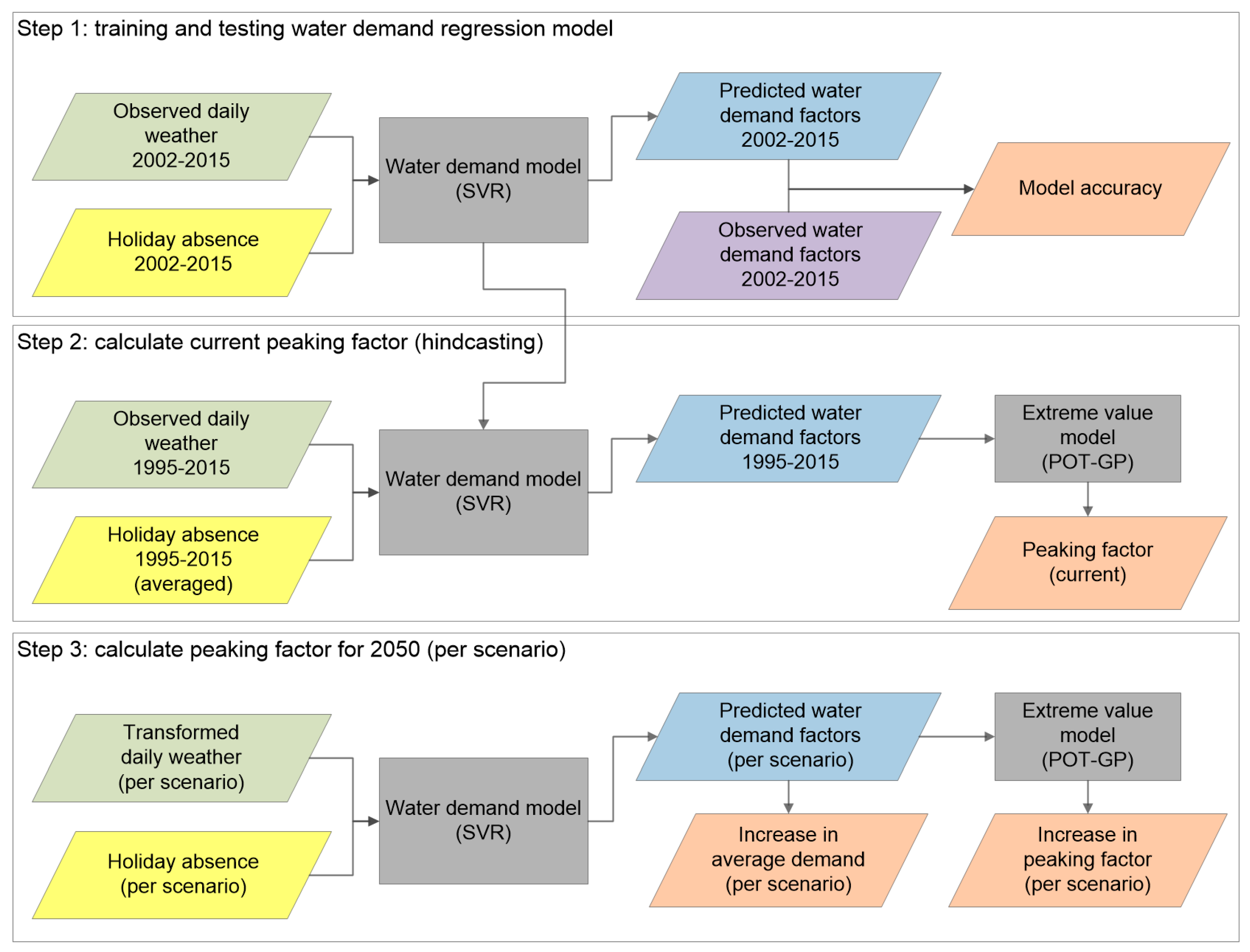
Our modeling framework consists of three distinct steps (Figure 1):
- Train and test a regression model that relates daily weather, vacation-related absence/presence and occurrence of national holidays to the measured drinking water demand. After initial training on observed (historical) drinking water demands, this model can be fed with climate-transformed weather patterns and different vacation scenarios in order to simulate corresponding water demand.
- Apply the regression model to a longer historical period to get homogeneous water demand time series representative for the current climate (hindcasting). Then use an extreme value model that samples peaks from the simulated water demand time series and fits those peaks to a statistical extreme value distribution. From this model the water demand factor corresponding with once in ten years occurrence can be extracted: The peaking factor.
- Finally, develop future scenarios (for horizon 2050 in our case) and use those to generate input time series for the regression model. Apply the regression and extreme value model on input time series for each scenario to obtain future peaking factors.
2.1.1. Regression Model
For (1) multiple model types are potentially suitable [10]. Researchers have reported using linear regression [18], artificial neural networks [19] or ARIMA models [11,18] for water demand forecasting problems. However, in our case we have some specific model requirements. Firstly, we specifically need to simulate peak demand correctly (as opposed to ‘regular demand’). Secondly, our model needs to handle extrapolation well. We will train our model on a historic time series of water demand, weather and vacation absence. Yet in the future, due to climate change, temperature may be higher than observed before. Even though by definition we cannot validate the model behavior on such yet-unobserved extremes, we require at least that the model be able to make realistic extrapolations in such circumstances. Finally, we will use some inputs that are known to have a non-linear relation with the output variable, such as air temperature (something also observed by others, for example by Sadiq and Karney [20]).
Considering the possibilities and limitations of various models, we chose to use a machine learning model called support vector regression (SVR). This regression model is based on the support vector machine (SVM) algorithm, which was initially developed for classification [21]. Generally speaking, SVRs are relatively insensitive to overfitting, which allows for good generalization of the model results [22]. The SVR algorithm tries to fit an arbitrary regression line on a dataset by minimizing the error between any data points that lie outside a predefined bandwidth ε around the regression line (Figure 2). This results in a convex quadratic optimization problem for which a global optimum can be derived [23]. In case of linear regression, the algorithm internally transforms input data through an inner product operation.
Input variables do however not need to be related to the output linearly: By transforming the input data with a so-called kernel function, non-linear relations can also be derived (the so-called ‘kernel trick’). In such non-linear cases, the inner product operation is replaced with a function that returns the inner product of lower dimensional data into a higher dimension. Common kernel functions are the polynomial, radial basis function (RBF) or sigmoid [24]. The polynomial kernel function is shown in Equation (1) and the RBF kernel in Equation (2):
In these equations and are input feature vectors, is the degree of the polynomial and is a free parameter that configures the sensitivity to differences in feature vectors. A commonly used default value of is the inverse of the number of features in the dataset [25].
The main hyperparameters of the SVR-model are C and ε and, in case of a RBF kernel, . C determines how much weight is given to a wrong prediction (error penalty) and ε is the size of the bandwidth around the regression function. We implemented the SVR-model using the Python-module Scikit-learn [25] and trained the model using 10-fold cross validation. To that extent, we randomly split the entire dataset from 2002–2015 into a subset for model selection (80%) and subset for model testing (20%). Optimal parameter values were derived using grid search.
2.1.2. Extreme Value Model
The actual peaking factor is calculated based on the water demand time series as simulated by the regression model. Two methods are common for sampling peaks from the time series: Block maxima (BM) and peak-over-threshold (POT). The BM method simply selects the highest peak from each year. Due to its simplicity, this is a frequently used method. A major disadvantage is however that a lot of data is not used in the analysis, in particular when multiple extremes occur in a year. For example, in years with two or three major demand peaks, by definition only the highest one is taken into account. The POT method solves this issue, by sampling all peaks that exceed a certain predefined threshold [26,27]. However, the method is more complicated as one needs to choose a suitable threshold for selecting peaks and additionally decluster the selected peaks to ensure that each peak is statistically independent of the other ones. This independence criterion, a prerequisite to any statistical frequency analysis [28], should be chosen such that a single extreme event is not counted multiple times. This is relevant in our case as water demand peaks regularly last multiple days. Without declustering, each individual day of the event would be considered as a separate peak, leading to an overestimation of its likelihood [29].
The dilemma when finding a suitable threshold is that a low threshold generates a lot of peaks, providing a lot of data for fitting an extreme-value distribution. This comes at the risk that the fitted distribution is at some point no longer an extreme-value distribution, since it includes relatively small peaks. A high threshold theoretically leads to the most accurate distribution at the cost of data loss. In our modeling framework we used a so called mean excess plot to select a suitable threshold [30]. Based on this plot, we determined the 99th percentile as a safe threshold, which we could automatically apply to each individual supply area.
For peak declustering, various criteria have been proposed. One could specify that two peaks are independent of each other if the water demand in between the peaks drops with a certain percentage, or alternatively define a criterion based on the time interval between subsequent peaks [28]. Regardless of which criterion is chosen, the question remains which exact value one should use. In practice, this is somewhat arbitrarily and often defined on a case-by-case basis, also considering the specific physics of the problem studied [28,30]. For its simplicity, we chose to use the time interval criterion and found an inter-peak interval of 5 days to be a safe limit for declustering daily water demand peaks. Thus, we required that a peak could only be counted as extreme if the previous 5 days did not contain any peak above the threshold. After this procedure, we ended up with on average about two sampled peaks per year.
We fitted the selected extremes on a generalized Pareto distribution [31]. Bayesian estimation was chosen as the optimization method for estimating the distribution parameters [32]. We used the R-package ‘extRemes’ [33] to perform these calculations. This package ingests time series and provides a set of sampling, model fitting and visualization methods that enables one to obtain the magnitude of peaks corresponding to various (extrapolated) return periods. From the fitted distribution, we derived the peaking factor corresponding to a 10 year return period.
2.1.3. Scenario Development
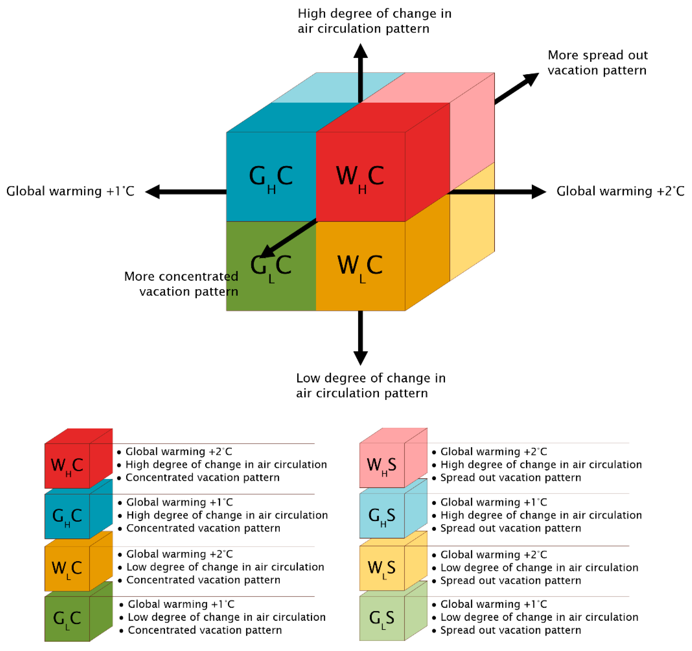
After initial model development and training, we developed eight different scenarios for 2050 (Figure 3). The scenarios include both climate change and vacation absence projections and are conceptually constructed along three axes of major uncertainty:
- The degree of change in air circulation patterns above the Netherlands and Flanders (small or large);
- The rise in global temperature (+1 °C or +2 °C compared to the 1990 baseline);
- The change in vacation absence patterns (more concentrated or more spread out throughout the year).
We used a transformation tool developed by the Royal Netherlands Meteorological Institute (KNMI) to transform the selected historical meteorological time series of 1995–2015 to the climate of 2050 [34]. The KNMI provides four standard climate scenarios [35], based on aforementioned axes of uncertainty (1) and (2). These scenarios are based on global IPCC projections, downscaled and tailored to the Dutch situation. The so-called GL and GH scenarios are on the lower side of the IPCC RCP4.5 and RCP6.0 range, and WL and WH are in the range of the RCP8.5. To reflect uncertain future development of vacation absence, we took the average pattern of 2002–2015 provided by the Central Statistics Bureau of the Netherlands (CBS) and respectively increased and decreased it with 25% (more concentrated tourism peaks versus more equally spread out tourism peaks).
2.2. Datasets
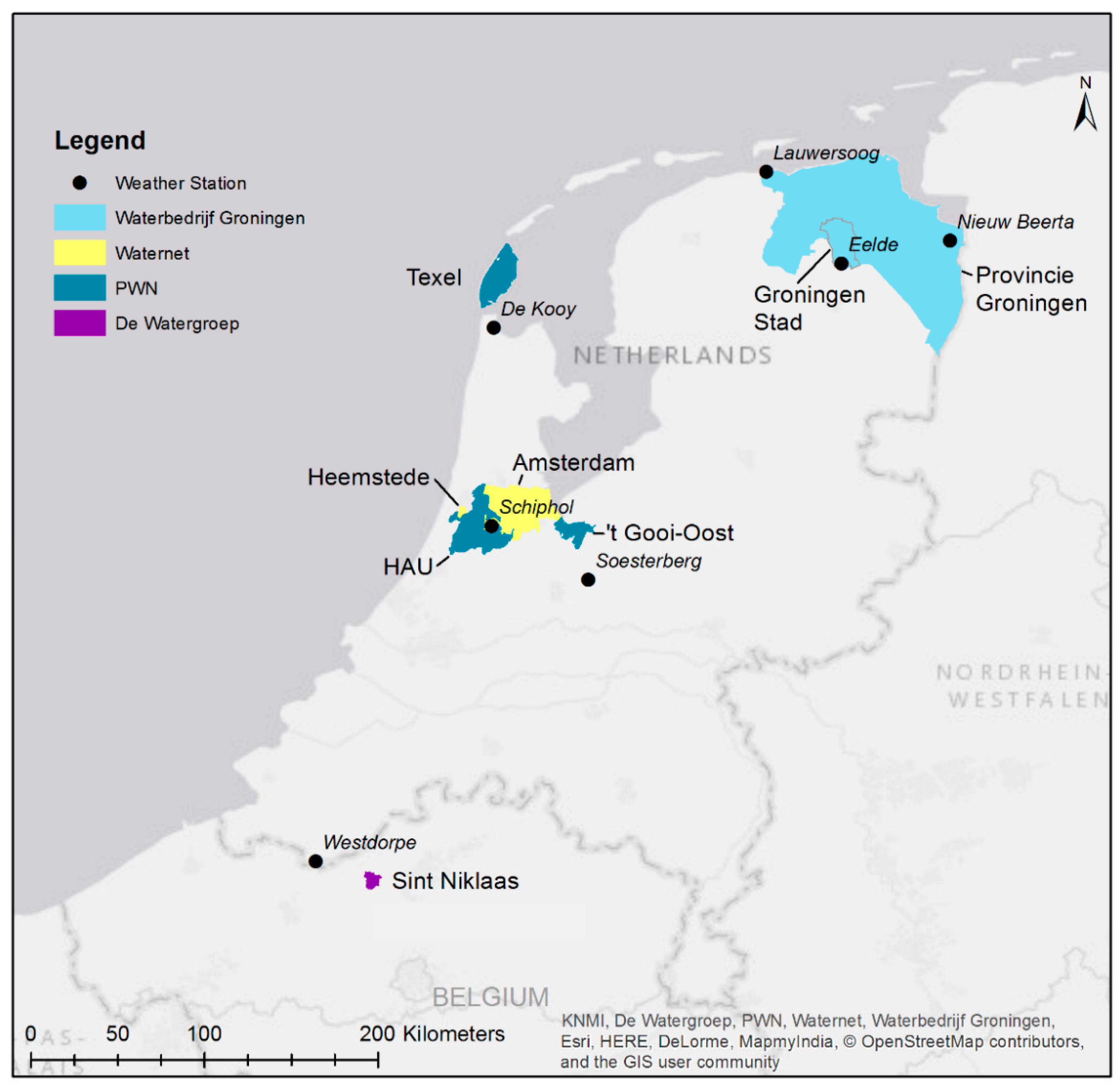
The location of the selected supply areas is shown in Figure 4. Four of these areas could be characterized as urban and four as suburban/rural. Texel is an island in the north of the Netherlands, well known as a summer tourist destination. Table 1 shows the main features of these areas. It could be observed that the demand per capita was highest on the island Texel. This was likely to be caused by the large presence of tourists during the holiday season (inflating the demand). Amsterdam had also a relatively high demand. Again a likely explanation was the constant high number of tourists in Amsterdam, artificially inflating the demand per capita.
2.2.1. Water Supply Records
Water utilities commonly keep record of daily water production at their abstraction and treatment works. Such records can be used as a fairly accurate proxy of actual water demand, under the condition that water losses (non-revenue water) are relatively small and fairly constant throughout the year.
With these constraints in mind, we could express daily drinking water demand as a ratio of the supplied volume on a certain day to the average daily supply in a given year. This ratio is often referred to as the demand factor. The peaking factor is defined as the demand factor with a certain return period in years, e.g., 10 years in the Netherlands [36]. Both factors allow drinking water utilities to compare variability of demand in different areas. In addition, such factors can be multiplied by the average daily demand in a certain year, to arrive at an absolute water volume for a particular day.
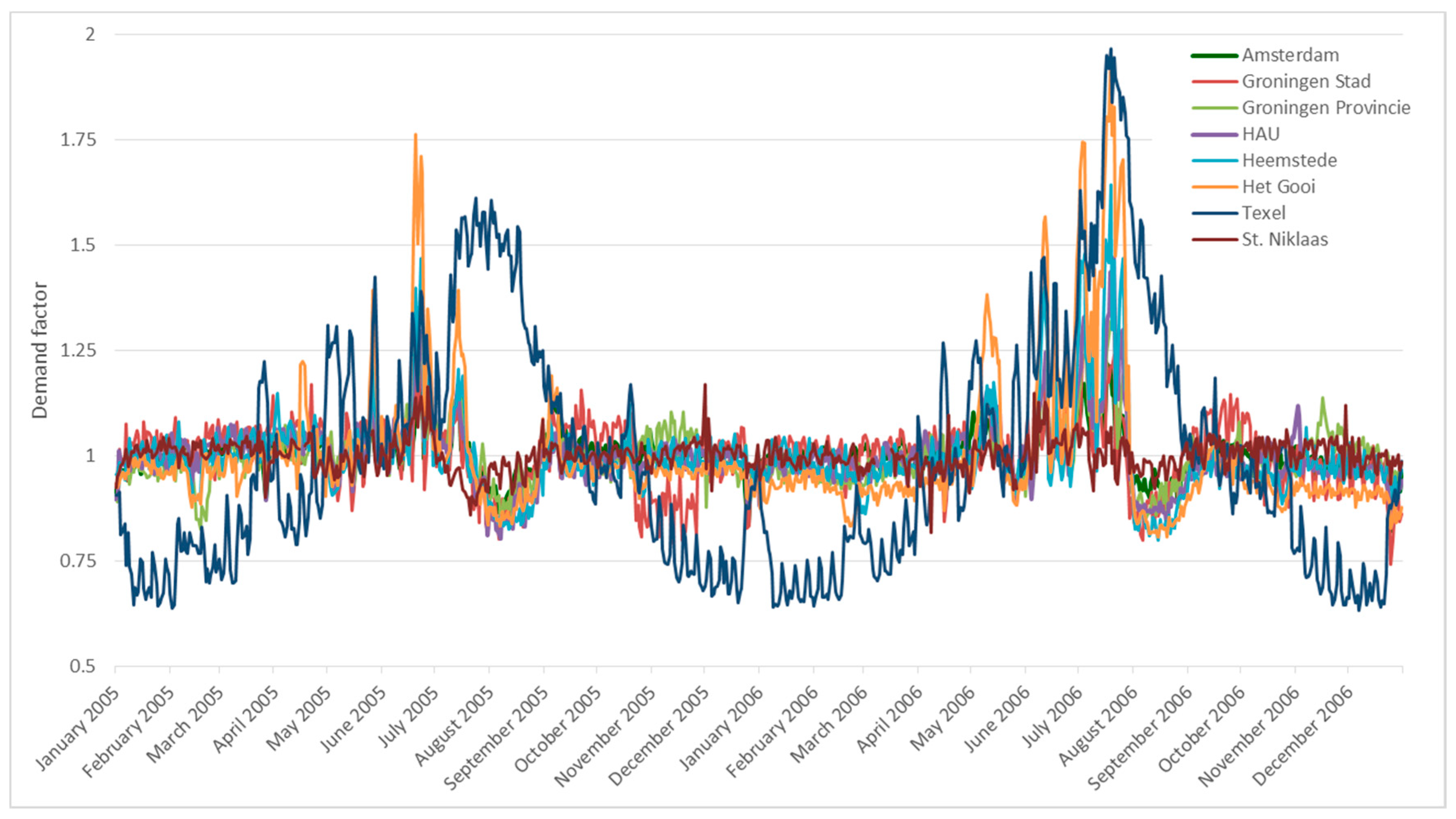
There are large differences in daily demand patterns between the selected supply areas (Figure 5). It can be observed that the areas Het Gooi and especially Texel have large water demand peaks. For most areas the ‘peak season’ started gradually in April, with the highest peaks around June/July and then an abrupt decrease around mid-July and August. In mostly residential areas many inhabitants were leaving for a vacation elsewhere during this period. Texel however showed a different pattern; instead of a decrease around the beginning of August, water demand increased. A likely explanation for this difference was the holiday season taking place around that period resulting in a large influx of tourists.
The obtained records contain some missing data. The gaps have been preserved and are ignored in the further modeling. Outliers were preserved unless operators could point to a specific technical or physical reason for their incorrectness, in which cases they were removed entirely from the supply record. Reason for preserving outliers is that we are specifically interested in peaks; removing extreme values purely on statistical grounds is likely to distort the analysis.
2.2.2. Meteorological Records
From the Dutch national meteorological service (KNMI), we obtained daily weather records. For each water supply area, data from the nearest meteorological station was used. In cases where multiple stations were located in the vicinity of a supply area, Thiessen-interpolation was used to derive spatially averaged time series. Table 2 gives an overview of meteorological parameters obtained for each supply area.
2.2.3. Vacation Absence Records
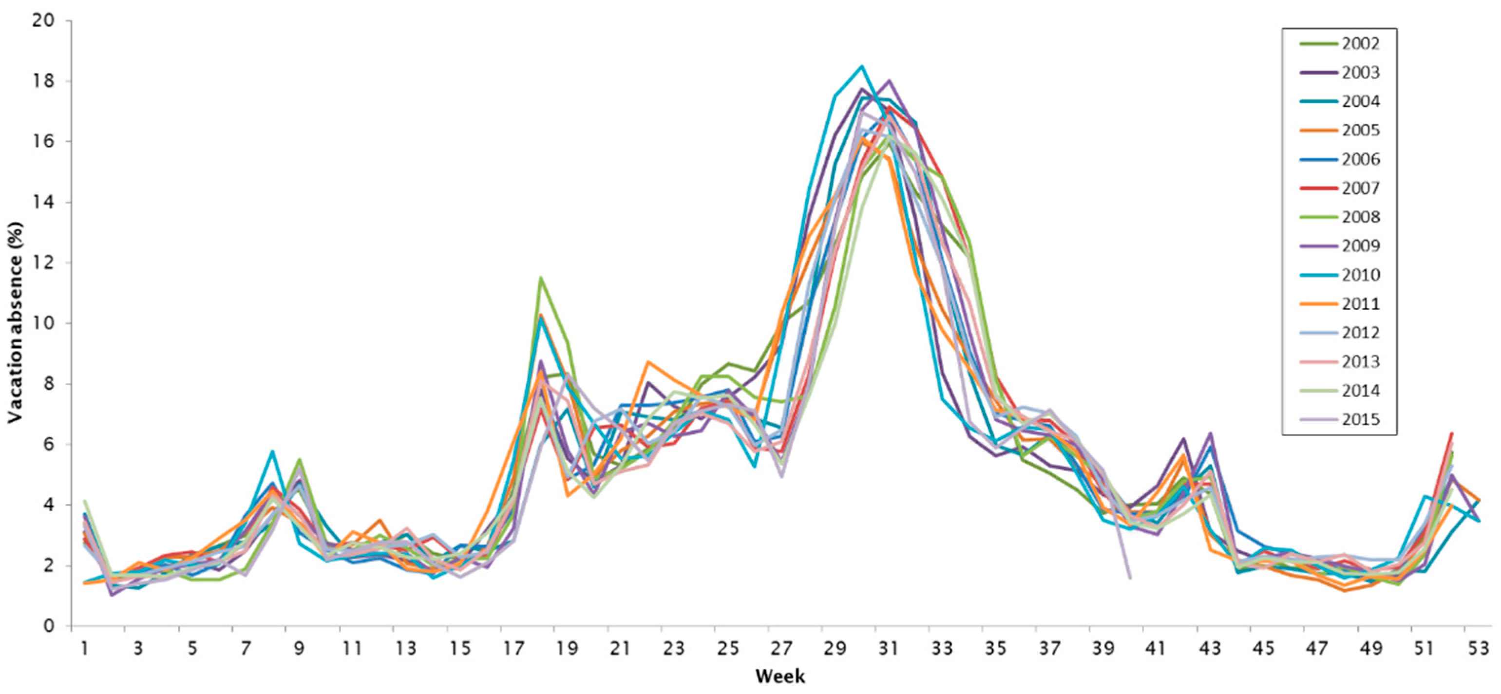
From the Central Statistics Bureau of the Netherlands (CBS) we obtained weekly statistics on the percentage of the population that is on vacation (Figure 6). These vacation absence records go back to 2002 [38] and are aggregated by the geographic region. The statistics are obtained through annual panel interviews (approximately 8700 participants), and are a good indicator for the absence of water consumers in non-touristic areas as well as the presence of additional water consumers in popular tourist destinations.
2.2.4. Other Data
To account for anomalous water consumption behavior on national holidays, we also included the national holiday calendars for Belgium and the Netherlands as input datasets for the model. The underlying rationale is that on national holidays some areas are likely to have a net influx of people attending large events, while other areas are likely to see a higher absence of people.
From the base datasets, we derived additional parameters, such as Boolean variables to indicate the month of the year and the type of day (weekend or weekday). As a long-term measure for the amount of drought, we calculated the cumulative precipitation deficit for the crop growth season (from the first of April till the first of October):
Here P is the daily precipitation in mm and E the daily evaporation in mm, both on day i. We expected this parameter to be an indicator for garden sprinkling.
Finally, we calculated the lagged values of all meteorological variables for the three days previous to the prediction date and added these to the input dataset. This allowed us to account for certain behavior of consumers, such as for example the decision to not sprinkle a garden on a hot day, if it has been raining in the past two days.
3. Results and Discussion
3.1. Regression Model
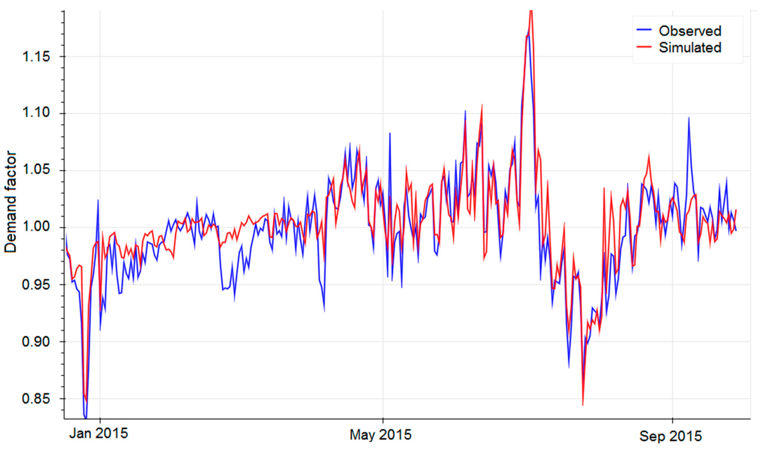
We trained and tested the regression model using the data from 2002–2015, eventually arriving at an architecture with a third-degree polynomial kernel. The often used RBF kernel gave similar results, but we found that the polynomial kernel stood out in accurately predicting the peaks in water demand, which is after all the most important aspect of this modeling framework. It can be observed that in general the training and test scores are in the same range (Table 3), which indicates a good generalization of the model. Area Sint Niklaas has a relatively low score for both training and testing, which can be attributed to poorer data quality for that area. After model training we assessed the simulations visually. We observed that in general peaks and valleys were simulated correctly. As an example, Figure 7 shows for supply area Amsterdam that noticeable lows (Christmas 2014) and peaks (July 2015) were simulated accurately. The small observed peak in September 2015 was caused by a major leak in the distribution network. This peak was correctly ignored by the model, as it is not the actual water demand but can be considered an artifact in the data.
3.2. Average Water Demand
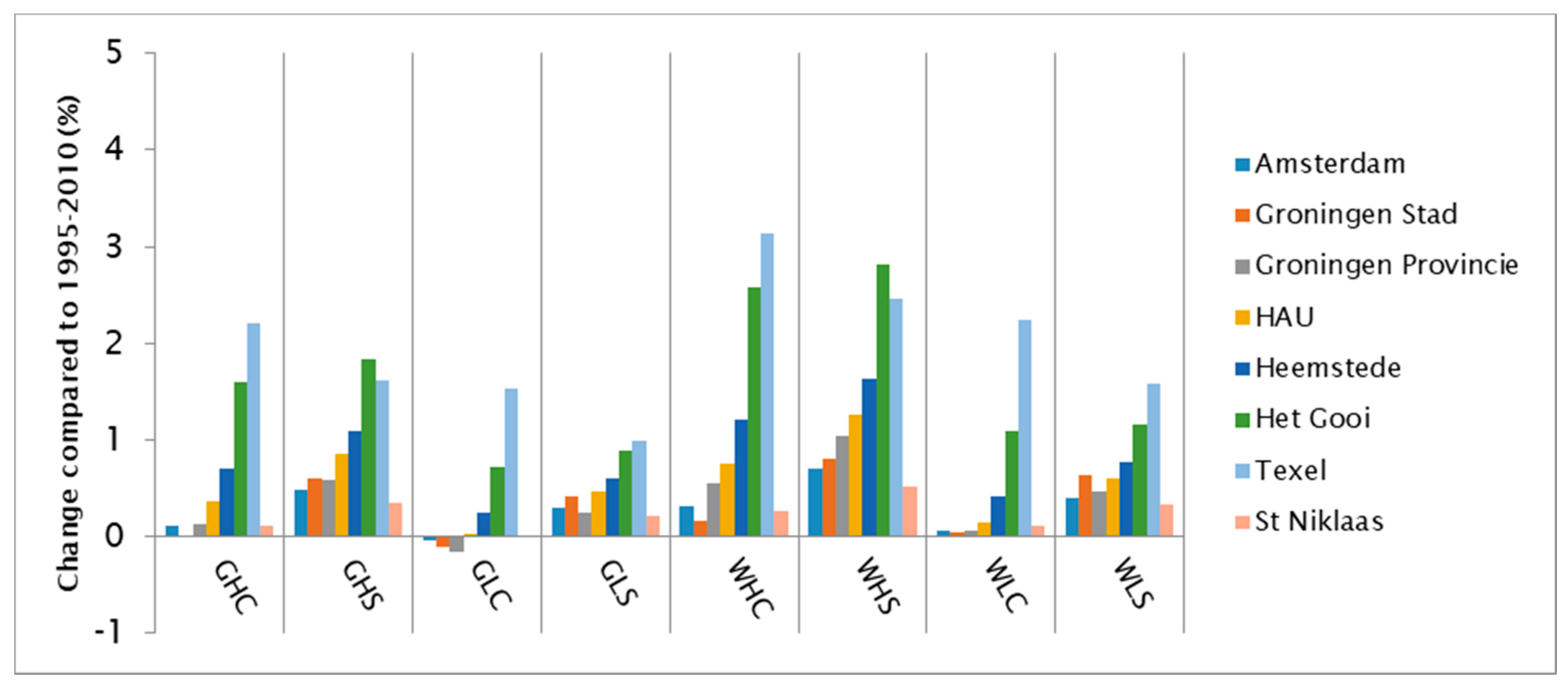
After training, validation and visual assessment, we applied the modeling framework to the eight water supply areas previously presented, and simulated the eight different future scenarios. This gives us an understanding of the sensitivity of water demand under various circumstances. It was found that on average there is a slight net increase in water demand with 0.8% in 2050. However, Figure 8 shows that between the different scenarios and supply areas the influence of climate change varies from −0.2% (GLC—Province of Groningen) to +3.1% (WHC—Texel).
There are noticeable differences between the investigated supply areas. On Texel, scenarios with a concentrated tourism peak consistently show a larger increase in average demand compared to their counterpart-scenarios with a spread out tourism peak. This illustrates the non-linearity of water demand: Even though all scenarios have the same number of tourists in total, water demand per capita varies throughout the year. In the ‘concentrated vacation’ scenarios most tourists visit in times that the water demand per capita is high (summer holiday period, with typically high temperatures). Hence, the total water demand also increases.
Somewhat oddly, supply areas Groningen Stad and Groningen Provincie show a decreasing demand in one of the scenarios (GLC). This can be attributed to the precipitation surplus, one of the input variables for the regression model, which is increasing for the northeastern part of the Netherlands whereas it is expected to decrease for the rest of the country.
3.3. Peaking Factor
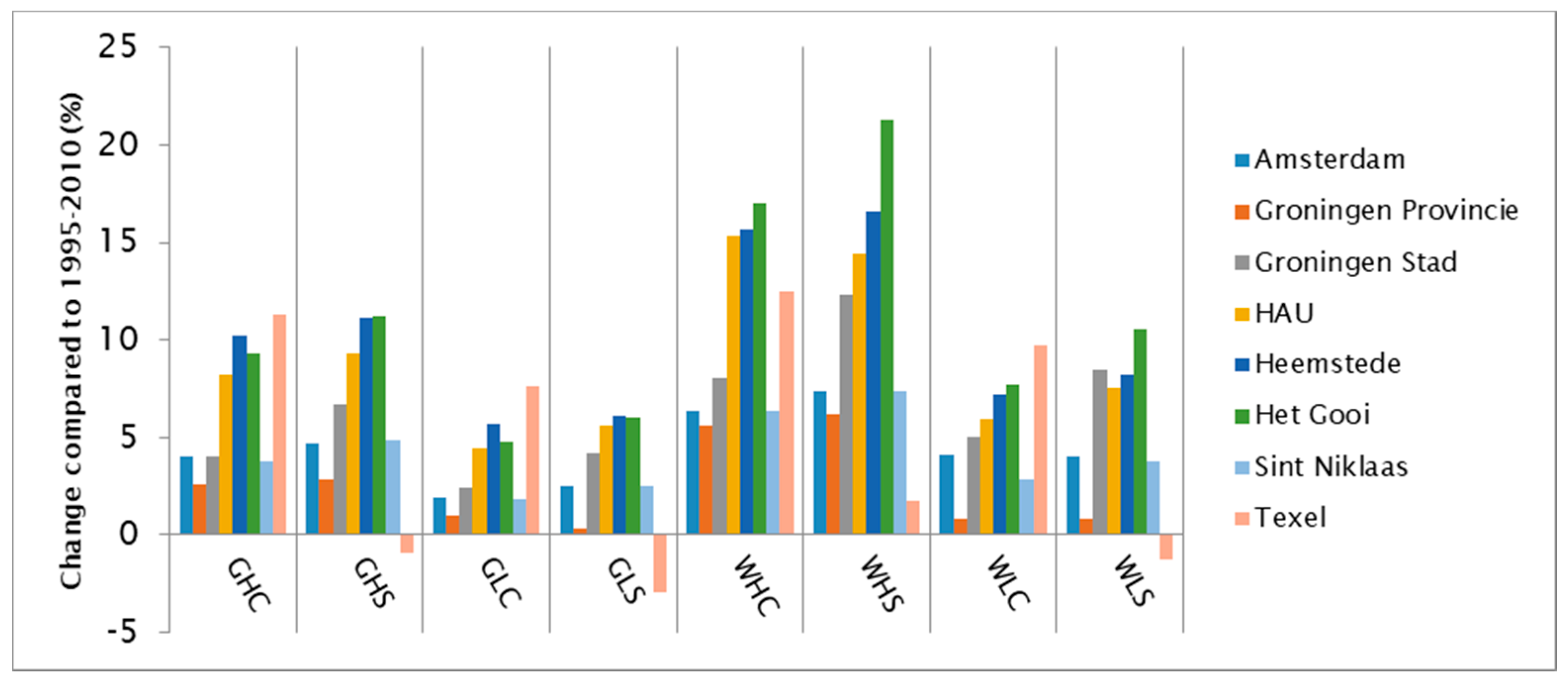
Whereas the average demand increased only slightly in the eight scenarios, the peaking factor shows a larger increase for most supply areas (Figure 9). The average increase in peak demand is 6.5% compared to the reference period, with the lowest value being −2.9% for Texel (GLS) and the largest increase being 21.3% (Het Gooi, scenario WHS). Table 4 shows the results for each area.
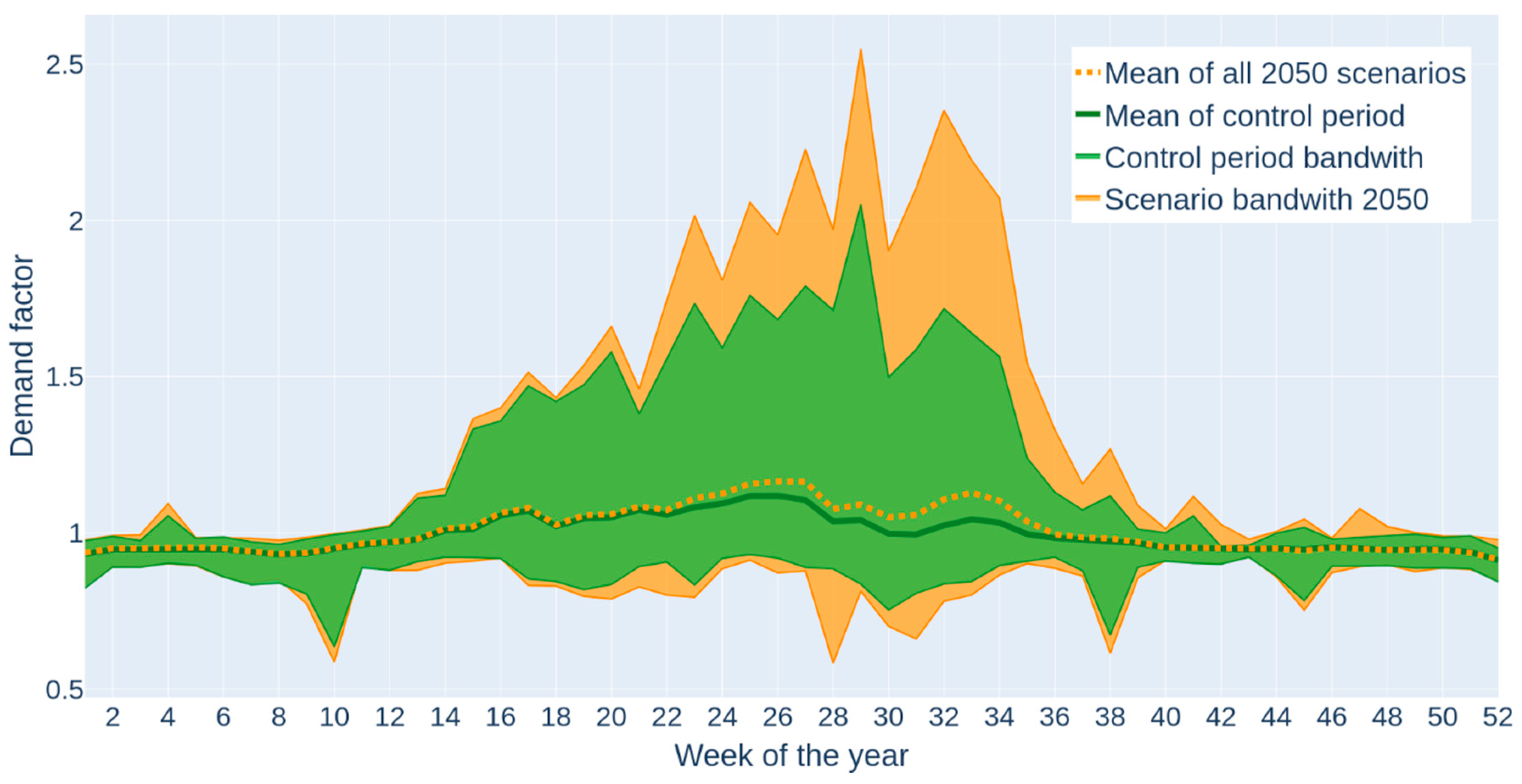
At Texel the peaking factor decreases in three of the four scenarios with a more spread out vacation pattern (the ‘S’-scenarios; Figure 9). Most other areas show an increased peaking factor for the spread out vacation scenarios. This can be explained with the timing of the peaks in the supply areas under study: Usually the highest demand peak occurs somewhere between week 26 and 34 (Figure 10), which is also exactly the period in which the summer vacation absence peaks. In short, if in that period less people are on vacation, the water demand peak becomes higher. The large differences in peak demand between scenarios with spread out vacations and scenarios with concentrated vacations shows just how important it is to include such statistics in these kinds of models. One would lose a lot of detail when simply assuming that vacation absence remains constant throughout the year, or accounting for major holidays with a simplified block signal.
4. Conclusions
The presented modeling framework allows for simulating water demand on long timescales with a temporal resolution of one day. It enables evaluation of the impact of climate change and variations in vacation absence on both the average daily water demand and the peaking factor. We showed the effectiveness of this model by applying it to eight different supply areas in the Netherlands and Belgium.
We found that the average demand increased somewhere between −0.2% and +3.1%, while the peaking factor increased between −2.9% and 21.3%. Thus we can conclude that variations in climate change and vacation absence affect the peaks in water demand much more than the averages. Even though these numbers are specific to the supply areas that we studied and to the scenarios that were used, they provided an estimate for the change that we might expect in the years to come, and at a minimum pinpoint an order of magnitude for the change.
The model results clearly show how climate change and variations in vacation absence could have surprisingly different impacts on different supply areas. This suggests that the choice of geographic scale is important in such analyses and that, in order for meaningful insights and outcomes to be obtained from such an assessment, it is crucial that relatively small geographic units of analysis are selected.
Results also highlight the importance of accounting for vacation absence (or vacation presence in tourist areas). The modeling framework is generic: It can be applied to any supply area as long as (a) distribution losses are fairly constant and low and (b) multiple years of historic daily water consumption data, vacation absence rates and weather observations are available.
Author Contributions
Conceptualization, D.G.C. and E.V.; Methodology, D.G.C. and E.V.; Software, E.V.; Validation, E.V., M.B. and D.G.C.; Formal analysis, E.V.; Investigation, E.V.; Data curation, E.V.; Writing—Original draft preparation, E.V.; Writing—Review and editing, D.G.C. and M.B.; Visualization, E.V.
Funding
This research was funded by the Dutch water utilities and De Watergroep.
Acknowledgments
This study was conducted as part of the joint research program (BTO) of the Dutch water utilities and De Watergroep. Authors want to thank PWN, Waterbedrijf Groningen, De Watergroep and Waternet for kindly providing historical water supply records.
Conflicts of Interest
The authors declare no conflict of interest.
References
- Zhang, X.; Buchberger, S.G.; van Zyl, J.E. A theoretical explanation for peaking factors. In Impacts of Global Climate Change, Proceedings of the World Water and Environmental Resources Congress 2005, Anchorage, AK, USA, 15–19 May 2005; American Society of Civil Engineers: Reston, VA, USA, 2005; pp. 1–12. [Google Scholar]
- Billings, R.B.; Jones, C.V. Forecasting Urban Water Demand; American Water Works Association: Denver, CO, USA, 2011. [Google Scholar]
- Murdock, S.H.; Albrecht, D.E.; Hamm, R.R.; Backman, K. Role of sociodemographic characteristics in projections of water use. J. Water Resour. Plan. Manag. 1991, 117, 235–251. [Google Scholar] [CrossRef]
- Wang, X.J.; Zhang, J.Y.; Shahid, S.; Guan, E.H.; Wu, Y.X.; Gao, J.; He, R.M. Adaptation to climate change impacts on water demand. Mitig. Adapt. Strateg. Glob. Chang. 2016, 21, 81–99. [Google Scholar] [CrossRef]
- Balling, R.C.; Gober, P.; Jones, N. Sensitivity of residential water consumption to variations in climate: An intraurban analysis of Phoenix, Arizona. Water Resour. Res. 2008, 44. [Google Scholar] [CrossRef] [Green Version]
- Donkor, E.A.; Mazzuchi, T.A.; Soyer, R.; Alan Roberson, J. Urban Water Demand Forecasting: Review of Methods and Models. J. Water Resour. Plan. Manag. 2014, 140, 146–159. [Google Scholar] [CrossRef]
- Alvisi, S.; Franchini, M.; Marinelli, A. A short-term, pattern-based model for water-demand forecasting. J. Hydroinform. 2007, 9, 39–50. [Google Scholar] [CrossRef] [Green Version]
- Bakker, M.; Van Duist, H.; Van Schagen, K.; Vreeburg, J.; Rietveld, L. Improving the Performance of Water Demand Forecasting Models by Using Weather Input. Procedia Eng. 2014, 70, 93–102. [Google Scholar] [CrossRef] [Green Version]
- Gardiner, V.; Herrington, P. Water Demand Forecasting; CRC Press: Boca Raton, FL, USA, 2014. [Google Scholar]
- Herrera, M.; Torgo, L.; Izquierdo, J.; Pérez-García, R. Predictive models for forecasting hourly urban water demand. J. Hydrol. 2010, 387, 141–150. [Google Scholar] [CrossRef]
- Zhou, S.L.; McMahon, T.A.; Walton, A.; Lewis, J. Forecasting daily urban water demand: A case study of Melbourne. J. Hydrol. 2000, 236, 153–164. [Google Scholar] [CrossRef]
- Cohen, S.J. Projected Increases in Municipal Water Use in the Great Lakes Due to CO2 induced Climatic Change. JAWRA J. Am. Water Resour. Assoc. 1987, 23, 91–101. [Google Scholar] [CrossRef]
- Goodchild, C.W. Modelling the Impact of Climate Change on Water Resources. Water Environ. J. 2003, 17, 8–12. [Google Scholar] [CrossRef]
- Babel, M.S.; Maporn, N.; Shinde, V.R. Incorporating future climatic and socioeconomic variables in water demand forecasting: A case study in Bangkok. Water Resour. Manag. 2014, 28, 2049–2062. [Google Scholar] [CrossRef]
- Toth, E.; Bragalli, C.; Neri, M. Assessing the significance of tourism and climate on residential water demand: Panel-data analysis and non-linear modelling of monthly water consumptions. Environ. Model. Softw. 2018, 103, 52–61. [Google Scholar] [CrossRef]
- Gössling, S.; Peeters, P.; Hall, C.M.; Ceron, J.P.; Dubois, G.; Scott, D. Tourism and water use: Supply, demand, and security. An international Review. Tour. Manag. 2012, 33, 1–15. [Google Scholar]
- Almutaz, I.; Ajbar, A.; Khalid, Y.; Ali, E. A probabilistic forecast of water demand for a tourist and desalination dependent city: Case of Mecca, Saudi Arabia. Desalination 2012, 294, 53–59. [Google Scholar] [CrossRef]
- Adamowski, J.; Fung Chan, H.; Prasher, S.O.; Ozga-Zielinski, B.; Sliusarieva, A. Comparison of multiple linear and nonlinear regression, autoregressive integrated moving average, artificial neural network, and wavelet artificial neural network methods for urban water demand forecasting in Montreal, Canada. Water Resour. Res. 2012, 48. [Google Scholar] [CrossRef]
- Ghiassi, M.; Zimbra, D.K.; Saidane, H. Urban water demand forecasting with a dynamic artificial neural network model. J. Water Resour. Plan. Manag. 2008, 134, 138–146. [Google Scholar] [CrossRef]
- Sadiq, W.A.; Karney, B.W. Modeling water demand considering impact of climate change—A Toronto case study. Eff. Model. Urban Water Syst. Monogr. 2005, 13. [Google Scholar] [CrossRef]
- Vapnik, V. The Nature of Statistical Learning Theory; Springer Science & Business Media: Berlin/Heidelberg, Germany, 2013. [Google Scholar]
- Auria, L.; Moro, R.A. Support Vector Machines (SVM) as a Technique for Solvency Analysis; Discussion Papers of DIW Berlin 811; DIW Berlin: Berlin, Germany, 2008. [Google Scholar]
- Smets, K.; Verdonk, B.; Jordaan, E.M. Evaluation of performance measures for SVR hyperparameter selection. In Proceedings of the 2007 International Joint Conference on Neural Networks, Orlando, FL, USA, 12–17 August 2007; IEEE: Piscataway, NJ, USA, 2007. [Google Scholar]
- Scholkopf, B.; Smola, A.J. Learning with Kernels: Support Vector Machines, Regularization, Optimization, and Beyond; MIT Press: Cambridge, MA, USA, 2001. [Google Scholar]
- Pedregosa, F.; Varoquaux, G.; Gramfort, A.; Michel, V.; Thirion, B.; Grisel, O.; Blondel, M.; Prettenhofer, P.; Weiss, R.; Dubourg, V.; et al. Scikit-learn: Machine learning in Python. J. Mach. Learn. Res. 2011, 12, 2825–2830. [Google Scholar]
- Faranda, D.; Lucarini, V.; Turchetti, G.; Vaienti, S. Numerical convergence of the block-maxima approach to the generalized extreme value distribution. J. Stat. Phys. 2011, 145, 1156–1180. [Google Scholar] [CrossRef]
- Ferreira, A.; de Haan, L. On the block maxima method in extreme value theory: PWM estimators. Ann. Stat. 2015, 43, 276–298. [Google Scholar] [CrossRef] [Green Version]
- Lang, M.; Ouarda, T.; Bobée, B. Towards operational guidelines for over-threshold modeling. J. Hydrol. 1999, 225, 103–117. [Google Scholar] [CrossRef]
- Kyselý, J.; Picek, J.; Beranová, R. Estimating extremes in climate change simulations using the peaks-over-threshold method with a non-stationary threshold. Glob. Planet. Chang. 2010, 72, 55–68. [Google Scholar] [CrossRef]
- Méndez, F.J.; Menéndez, M.; Luceño, A.; Losada, I.J. Estimation of the long-term variability of extreme significant wave height using a time-dependent peak over threshold (pot) model. J. Geophys. Res. Ocean. 2006, 111. [Google Scholar] [CrossRef]
- Renard, B.; Lang, M.; Bois, P. Statistical analysis of extreme events in a non-stationary context via a Bayesian framework: Case study with peak-over-threshold data. Stoch. Environ. Res. Risk Assess. 2006, 21, 97–112. [Google Scholar] [CrossRef]
- Martins, E.S.; Stedinger, J.R. Generalized maximum-likelihood generalized extreme-value quantile estimators for hydrologic data. Water Resour. Res. 2000, 36, 737–744. [Google Scholar] [CrossRef]
- Gilleland, E.; Katz, R.W. extRemes 2.0: An extreme value analysis package in R. J. Stat. Softw. 2016, 72, 1–39. [Google Scholar]
- Bakker, A. Time Series Transformation Tool Version 3.1—Description of the Program to Generate Time Series Consistent with the KNMI’14 Climate Scenarios; KNMI: De Bilt, The Netherlands, 2015. [Google Scholar]
- Van Den Hurk, B.; Siegmund, P.; Tank, A.K. KNMI’14: Climate Change Scenarios for the 21st Century—A Netherlands Perspective; KNMI: De Bilt, The Netherlands, 2014. [Google Scholar]
- Van Dijk Hans, J.; QJC, V.J.; De Moel Peter, J. Drinking Water: Principles and Practices; World Scientific: Singapore, 2006. [Google Scholar]
- Rijtema, P. Calculation Methods of Potential Evapotranspiration; ICW: Glasgow, UK, 1959. [Google Scholar]
- CBS. Continu Vakantie Onderzoek (CVO). 2019. Available online: https://www.cbs.nl/nl-nl/onze-diensten/methoden/onderzoeksomschrijvingen/korte-onderzoeksbeschrijvingen/continu-vakantie-onderzoek--cvo---tot-2017 (accessed on 20 May 2019).
Figure 1.
Modeling framework workflow.

Figure 2.
Support vector regression concept illustrated. In this simplified example, the algorithm fits a regression line through a collection of points by minimizing the number of points that falls outside the bandwidth (defined by parameter ε). Each point outside the bandwidth is penalized according to a penalty weight C.

Figure 3.
Overview of scenarios simulated in this study.

Figure 4.
Locations of supply areas studied in this research. Colors represent the different utilities managing the supply areas.
Figure 4.
Locations of supply areas studied in this research. Colors represent the different utilities managing the supply areas.

Figure 5.
Demand patterns during the years 2005 and 2006 for the supply areas. It can be observed that Texel has a very distinct demand pattern, with a clear peak in the holiday around July and August. In the other supply areas, higher peaks start to occur around May and build up in magnitude to the end of July.

Figure 6.
Weekly vacation absence patterns for the West region of the Netherlands (2002–2015) based on Central Statistics Bureau of the Netherlands (CBS) data.
Figure 6.
Weekly vacation absence patterns for the West region of the Netherlands (2002–2015) based on Central Statistics Bureau of the Netherlands (CBS) data.

Figure 7.
Simulated (red) and measured (blue) water demand factor in Amsterdam for September 2014–October 2015.
Figure 7.
Simulated (red) and measured (blue) water demand factor in Amsterdam for September 2014–October 2015.

Figure 8.
Change in average water demand. The projected increase differs with a few percent between the different areas and scenarios considered. However, the increase in average water demand is in all cases smaller than 3.1%.
Figure 8.
Change in average water demand. The projected increase differs with a few percent between the different areas and scenarios considered. However, the increase in average water demand is in all cases smaller than 3.1%.

Figure 9.
Change in peak water demand. By comparing differences between the ‘S’ and ‘C’ version of each scenario, it becomes clear that vacation absence has a large influence on the increase in the peaking factor. This is particularly true for Texel, which shows completely different demand peaks depending on how tourist visits are spread in time.

Figure 10.
Water demand regime for supply area Het Gooi for the control period and 2050 scenarios. The winter period can be characterized as being relatively stable in terms of variability in demand, whereas the summer season shows high variability.
Figure 10.
Water demand regime for supply area Het Gooi for the control period and 2050 scenarios. The winter period can be characterized as being relatively stable in terms of variability in demand, whereas the summer season shows high variability.


Table 1.
Main characteristics of supply areas. Statistics apply to the year 2015.
| Supply Area | Number of Inhabitants (×1000) | Type | Average Demand (×1000 m3/d) | Average Demand Per Capita (m3/d) | Water Utility |
|---|---|---|---|---|---|
| Amsterdam | 955 | Urban | 191 | 0.20 | Waternet |
| Groningen Provincie | 394 | Suburban/rural | 91 | 0.23 | Waterbedrijf Groningen |
| Groningen Stad | 198 | Urban | 33 | 0.17 | Waterbedrijf Groningen |
| HAU | 215 | Suburban | 39 | 0.18 | PWN |
| Heemstede | 26 | Urban | 4 | 0.15 | Waternet |
| Het Gooi | 112 | Rural | 20 | 0.18 | PWN |
| Texel | 14 | Rural | 4 | 0.29 | PWN |
| Sint Niklaas | 51 | Urban | 7 | 0.14 | De Watergroep |
Table 2.
Meteorological parameters.
| Variable | Unit | Description |
|---|---|---|
| P | mm | Precipitation |
| E | mm | Reference evaporation according to Makkink [37] |
| Tav | °C | Average daily temperature |
| Tmax | °C | Maximum daily temperature |
| Q | J/cm2 | Solar irradiance |
Table 3.
Model training and test results for each supply area.
| Supply Area | C | R2 Training | R2 Test | |
|---|---|---|---|---|
| Amsterdam | 0.022 | 0.018 | 0.70 | 0.63 |
| Groningen Provincie | 0.05 | 0.022 | 0.72 | 0.66 |
| Groningen Stad | 0.12 | 0.04 | 0.60 | 0.50 |
| HAU | 0.025 | 0.034 | 0.62 | 0.60 |
| Heemstede | 0.04 | 0.027 | 0.60 | 0.61 |
| Het Gooi | 0.10 | 0.020 | 0.80 | 0.77 |
| Texel | 0.14 | 0.038 | 0.93 | 0.91 |
| Sint Niklaas | 0.019 | 0.013 | 0.44 | 0.39 |
Table 4.
Bandwidth of projected peaking factor change per supply area.
| Supply Area | Peaking Factor Current | Peaking Factor 2050 (Min–Max) | Relative Change (%, Min–Max) |
|---|---|---|---|
| Amsterdam | 1.19 | 1.21–1.28 | 1.7–7.6 |
| Groningen Provincie | 1.30 | 1.30–1.38 | 0–6.2 |
| Groningen Stad | 1.21 | 1.24–1.36 | 2.5–12 |
| HAU | 1.34 | 1.40–1.54 | 4.5–15 |
| Heemstede | 1.50 | 1.58–1.75 | 5.3–16.7 |
| Het Gooi | 1.90 | 1.99–2.31 | 4.7–21.6 |
| Texel | 1.99 | 1.93–2.24 | −3–12.6 |
| Sint Niklaas | 1.15 | 1.17–1.24 | 1.7–7.8 |
© 2019 by the authors. Licensee MDPI, Basel, Switzerland. This article is an open access article distributed under the terms and conditions of the Creative Commons Attribution (CC BY) license (http://creativecommons.org/licenses/by/4.0/).
Share and Cite
MDPI and ACS Style
Vonk, E.; Cirkel, D.G.; Blokker, M. Estimating Peak Daily Water Demand under Different Climate Change and Vacation Scenarios. Water 2019, 11, 1874. https://doi.org/10.3390/w11091874
AMA Style
Vonk E, Cirkel DG, Blokker M. Estimating Peak Daily Water Demand under Different Climate Change and Vacation Scenarios. Water. 2019; 11(9):1874. https://doi.org/10.3390/w11091874
Chicago/Turabian StyleVonk, Erwin, Dirk Gijsbert Cirkel, and Mirjam Blokker. 2019. "Estimating Peak Daily Water Demand under Different Climate Change and Vacation Scenarios" Water 11, no. 9: 1874. https://doi.org/10.3390/w11091874
Note that from the first issue of 2016, this journal uses article numbers instead of page numbers. See further details here.