Algae Growth Distribution and Key Prevention and Control Positions for the Middle Route of the South-to-North Water Diversion Project

1
College of Architecture and Civil Engineering, Beijing University of Technology, Beijing 100124, China
2
China Institute of Water Resources and Hydropower Research, Beijing 100038, China
*
Author to whom correspondence should be addressed.
Water 2019, 11(9), 1851; https://doi.org/10.3390/w11091851
Submission received: 9 July 2019
/
Revised: 8 August 2019
/
Accepted: 3 September 2019
/
Published: 5 September 2019
(This article belongs to the Special Issue Biomonitoring of Water Quality)
Abstract
:The Middle Route of the South-to-North Water Diversion Project (MRP) is an important water supply for 20 large cities and 100 counties in Northern China. However, since 2016, the growth of large filamentous algae clusters has threatened the safety of the main canal water supply and water quality. In this study, a field investigation, monitoring, and hydrodynamic simulation were performed to analyze the hydrodynamic habitat conditions in areas with vigorous algae growth and establish a relationship between the hydrodynamic habitat conditions of the main canal and the growth, distribution, and correlation of macrobenthic algae in the main canal. The results showed that: (1) algae zones in the main canal are more likely to appear along curves, and the largest algal zone was at the front of the large curved section; (2) the length of the algae growth zone is related to the flow rate; and (3) a lower flow velocity in the main canal facilitates faster growth of an algae zone. This study provides specific and effective suggestions for the key prevention and control positions, which has important guidance on improving the efficiency of algae control in the main canal.
1. Introduction
The Middle Route of the South-to-North Water Diversion Project (MRP) was completed in 2014 and diverts water from the Danjiangkou Reservoir in the Hanjiang River Basin to 20 large cities and 100 counties in Henan and Hebei Provinces and Beijing and Tianjin Municipalities [1]. The MRP has complex hydraulic structures in a long canal and provides drinking water in open and covered channels to Beijing and Tianjin, meeting extremely strict water quality requirements, which has led to significant challenges [2,3]. The completion of the MRP provided a reliable water supply for water-scarce cities to alleviate the tight supply of water resources and has played a huge role in the sustainable socioeconomic development and improvement of the ecological environment in this area.
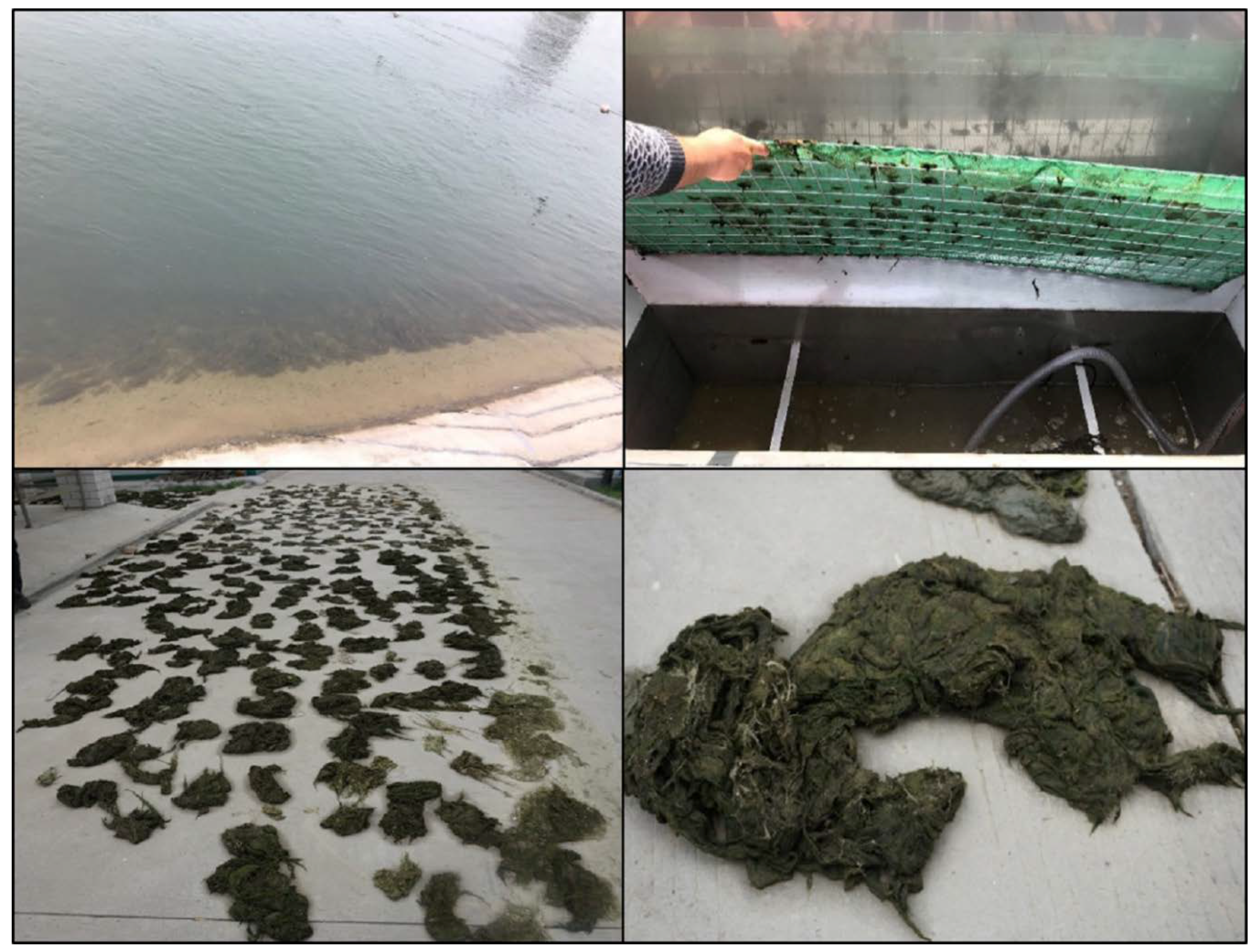
However, since 2016, rapid algae growth has occurred in areas of the main canal of MRP in the spring and autumn, and the large number of filamentous algae clusters in the main canal has caused problems such as blockages of the watershed grilles and rapid siltation before the exit sluice; this has threatened the safety of the water supply and influenced the grade of water quality (see Figure 1). At present, there is a lack of monitoring data and insufficient research has been conducted on these algae problems in the main canal. Investigations of algae growth areas are urgently needed to determine the source of the algae and analyze the key factors that affect algae growth in the main canal in order to develop scientific and effective strategies for dealing with abnormal algae proliferation.
Although the growth mechanism of algae is very complicated, many studies have shown that it is closely related to the water level, flow rate, water temperature, amount of light, and water quality [4,5,6]. The main environmental conditions necessary for the growth and reproduction of specific dominant algae are basically similar [7]: plentiful nutrients, such as nitrogen and phosphorus, suitable hydrological conditions, as well as favorable climatic conditions. These three conditions must be satisfied for abnormally dominant algae blooms to occur. In recent years, scholars have conducted many studies on algae communities [8], considering different regional climates (temperate, subtropical, and changing), types of aquatic ecosystems (lakes, coastal wetlands, swamps, glaciers, and rivers), river states (still, rapids), and epiphytic algae in water bodies with different nutrient structures [9]. These studies mostly focused on the characteristics of the algae community structure, changes in the time and space domains, and the relationship between related abiotic impact factors and living algae [10,11].
An increasing number of studies have focused on the effects of hydrodynamic conditions on algae growth. The hydrodynamic process is one of the most important factors that affect the eutrophication status of water bodies and algae reproduction, and there are significant differences in the hydrodynamic effects of water as caused by lake circulation and river runoff [12,13,14]. Algae growth is affected by the hydrodynamic process in terms of both the flow rate and flow state [15]. There is a critical flow rate that maximizes chlorophyll concentration, and different algae have different critical flow rates. According to Jiao [16], the critical velocity for an algal bloom outbreak is about 0.05 m/s, that for Chlorella growth is about 0.05 m/s, and that for filamentous algae is about 0.01 m/s. The flow velocity has little effect on the growth of Scenedesmus and Anabaena. For the flow state, algae growth is inhibited when the degree of turbulence increases, but the flow regimes (laminar, transitional, and turbulent) do not have a significant association with this inhibition. The results obtained by Hondzo [17] showed that, when the Reynolds number ranged from 0 to 2350 (the Reynolds number is a dimensionless number used to characterize fluid flow) the growth inhibition of Scenedesmus quadricauda was most obvious due to the change in the flow pattern. When the Reynolds number increased to 8500, the growth rate was not affected. In static water, the growth of Scenedesmus quadricauda was at its maximum.
Ding et al. [18] found that the flow rate can affect the proportions of periphytic algae and phytoplankton: a slower flow rate leads to a smaller diatom biomass and the dominance of periphytic algae, while a faster flow rate leads to a larger diatom biomass and a dominance of planktonic diatoms. However, Ding et al. [19] found that the scouring action of the water flow can both promote and inhibit the proliferation of algae. A slow flow rate promotes proliferation, while a high flow rate inhibits proliferation. A high flow rate has an adverse effect on the initial stage of algae formation but is subsequently beneficial to the proliferation of filamentous algae. Wang et al. [20] derived an exponential relationship between algae growth and the reciprocal of the flow rate for the Hanjiang River and determined that the critical flow rate for an algae bloom in this section is 0.225 m/s. Li et al. [21] increased the hydrodynamic influence factor and obtained a linear relationship between the influence of the hydrodynamic conditions and the algae growth rate in the tributaries of the Three Gorges Reservoir area by applying a numerical fitting analysis. Huang [22] found that the flow rate in the backwater area of the Daning River has a significant negative correlation with algae. Borchardt [23] concluded that the flow rate does not affect the respiration rate of the algae but does affect the absorption capacity of carbon in photosynthesis, which increases with the flow rate. The water flow reduces the amount of stagnant water around the algae cells and increases the diffusion and absorption of nutrients. Healey [24] proposed that the water flow affects the growth of algae by changing the light intensity and water temperature. Pannard [25] proposed that a high flow rate leads to the suspension of sediments and that the resettling process has an effect akin to tape-wrapping on the algae; this causes some algae to lose buoyancy and settle, which reduces the number of phytoplankton. Huisman [26] showed that disturbances affect the competition between different algae for light, which may affect floating algae. Weak disturbances help Microcystis become the dominant species, while strong disturbances make diatoms and green algae the dominant species.
During the planning stage, MRP was positioned as an auxiliary water source for each water-receiving area. However, the development of the economy, population, industry, and agriculture in each water-receiving area gradually increased the urban water demand, such that MRP gradually changed from an auxiliary water source to a main water source. Therefore, it is particularly important to investigate those areas with vigorous algae growth and determine the source of algae in order to analyze the key factors that affect algae growth, while addressing the lack of algae monitoring in the main canal as well as the need for related research.
Based on the results of previous research, this study focused on the abnormal proliferation of algae in the main canal and its threat to the operation of MRP. A field survey, monitoring, and hydrodynamic simulation were performed to analyze the hydrodynamic habitat conditions in areas with high algae growth. The conditions in the main canal and the growth, distribution, and correlation of macrobenthic algae in the main canal were established to support the prevention and control of abnormal algae proliferation in the main canal.
2. Materials and Methods
2.1. Study Area
MRP took more than 60 years to complete from its proposal (30 October 1952), through exploration, measurement, planning, design, and construction. The main components are the water source area, the main canal for water diversion, and supporting projects in the water receiving area. MRP has the following basic characteristics:
- Long water delivery route: The total length of the main canal is 1432 km. The length from the head of the main canal to the south of the middle branch north of the Juma River is 1196.51 km, and an open canal is used for water diversion. A prestressed concrete cylinder pipe (PCCP) and underground culvert are used for water diversion in the Beijing section which has a total length of 80.05 km. The Tianjin water diversion branch line has a length of 155 km, and an underground culvert is used for the water diversion.
- Large-scale water diversion: The average annual water transfer of the MRP is 9.5 billion m3. For the main canal control points, Taocha has a design flow of 350 m3/s and an enlarged flow of 420 m3/s, while the head of the Tianjin main canal has a design flow of 50 m3/s and an enlarged flow of 60 m3/s. With regard to the general principle of water head distribution in the main canal, the design water levels of Taocha and Beijing Tuancheng Lake are taken as the control. The total water head is distributed among the open canals and buildings on both sides of the Yellow River. The main canal has a total water head of 98.81 m. The water heads are 29.38 m south of the Yellow River and 59.43 m north of the Yellow River. The section from Taocha to north of the Juma River uses an open canal to divert water and has a total water head of 87.08 m.
- Numerous buildings: the MRP has more than 1750 hydraulic structures of various types, including 97 diversion gates, 64 check gates, 54 exit sluices, 61 control gates, nine tunnels, and one pump station.
- Strict water-quality requirements: The main purpose of the MRP is to supply water for consumption and industry in areas with scarce water resources. Therefore, the water quality needs to satisfy the Type II requirements of China’s environmental quality standard for surface water (GB3838-2002).
More than 53.1 million residents drink water from the MRP: 11 million in Beijing Municipality, 9 million in Tianjin Municipality, 15.1 million in Hebei Province, and 18 million in Henan Province. At present, MRP provides more than 70% of the urban water supply in the Beijing Municipality and has increased the per capita water resources in the city from 100 m3 to 150 m3 and the water supply safety factor in the central city from 1.0 to 1.2. It provides 100% of the urban water supply in the Tianjin Municipality, with the residents of 14 administrative regions obtaining their drinking water from the MRP.
In the past four years, the MRP has effectively improved the water supply safety factor of the Beijing and Tianjin Municipalities, Hebei Province, and the surrounding cities. The water quality available to residents has significantly improved. The water shortages in those cities along the line have been effectively alleviated, and the ecological environment has been improved. MRP has played an important role in ensuring water security, rehabilitating the water ecology, improving the water environment, and optimizing water resource allocation. It has brought great social, economic, and ecological benefits [27].
2.2. Field Investigation and Model Building
2.2.1. Field Investigation
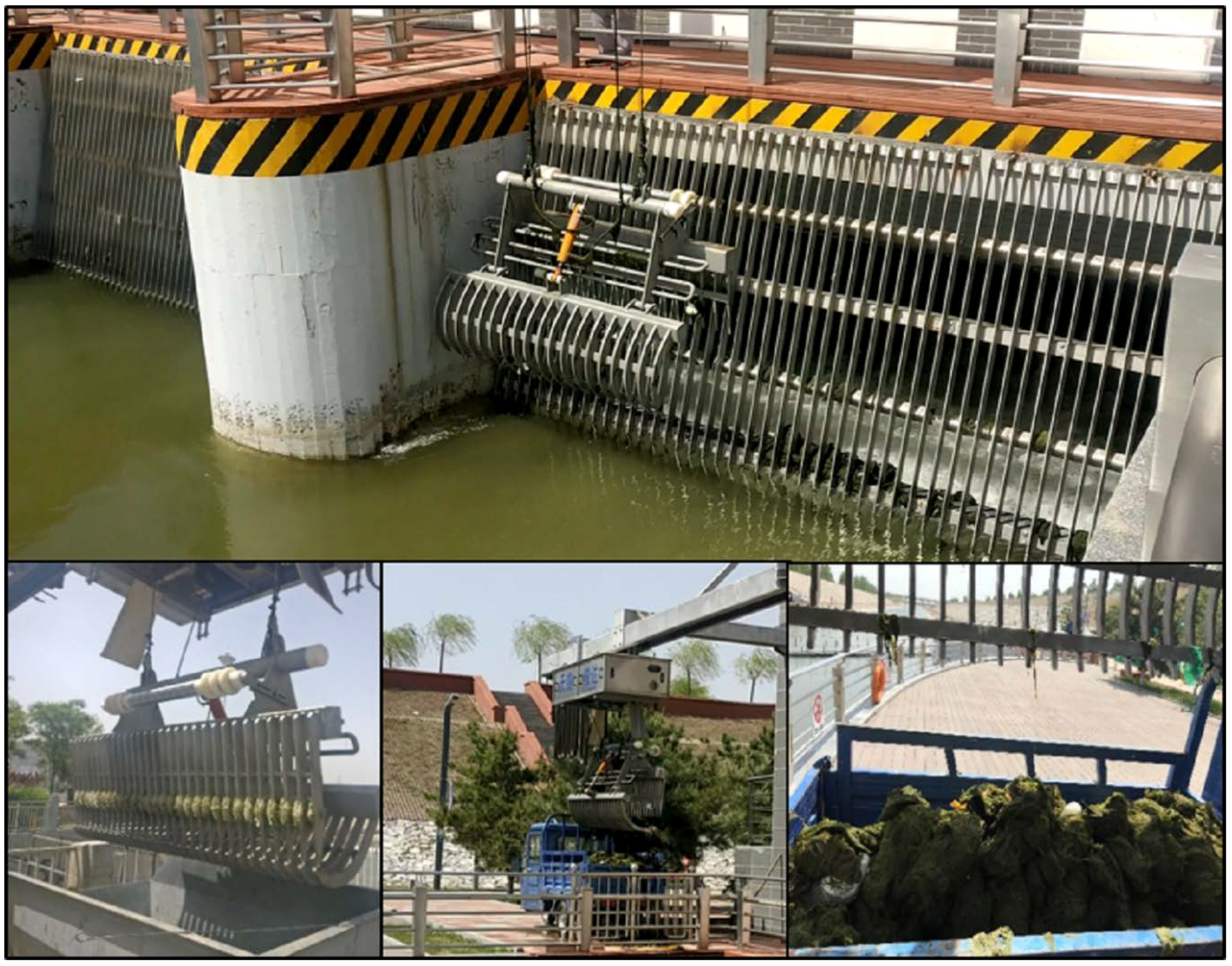
A one-year field survey was performed on algae in the main canal of MRP in 2018 to investigate areas of vigorous algae growth, the length of the algae growth zone (hereinafter referred to as an algae zone), and the algae source. In the spring, the results showed that the main canal contained benthic algae of the genus Chladophora (Chlorophyta, Cadophorales) [28]. It is a filamentous, green branching algae. It takes the form of a filamentous ball when it gathers and grows. It does not feel slippery when touched, and the filament feels hard and thin. The outbreak period of this algae growth is mainly from late March to early June. Before the onset of the algae outbreak period, the cleaning frequency of the algae traps at the water diversion outlets or control gates was twice every 2 or 3 days, and the amount of algae caught was small. After the onset of the algae outbreak, however, the amount of algae in the main canal gradually increased. The cleaning frequency of the traps was as high as five times a day, and the amount of algae caught increased sharply. An average of eight vehicles a day were needed for cleaning, with each vehicle carrying away approximately 400 kg of algae including the weight of water, as shown in Figure 2. In the autumn, field sampling and identification showed that the algae attached to the main canal walls were Spirogyra communis (Charophyta, Zygnematales), while the Cladophora had basically died or become dormant. Spirogyra communis is a green algae that was found to wind around the remnants or root surfaces of Cladophora, which is quite different from the observations made in the spring. This indicates that the species, growth, distribution characteristics, and attachment mechanisms of the algae adhering to the walls of the main canal differed between the spring and autumn.
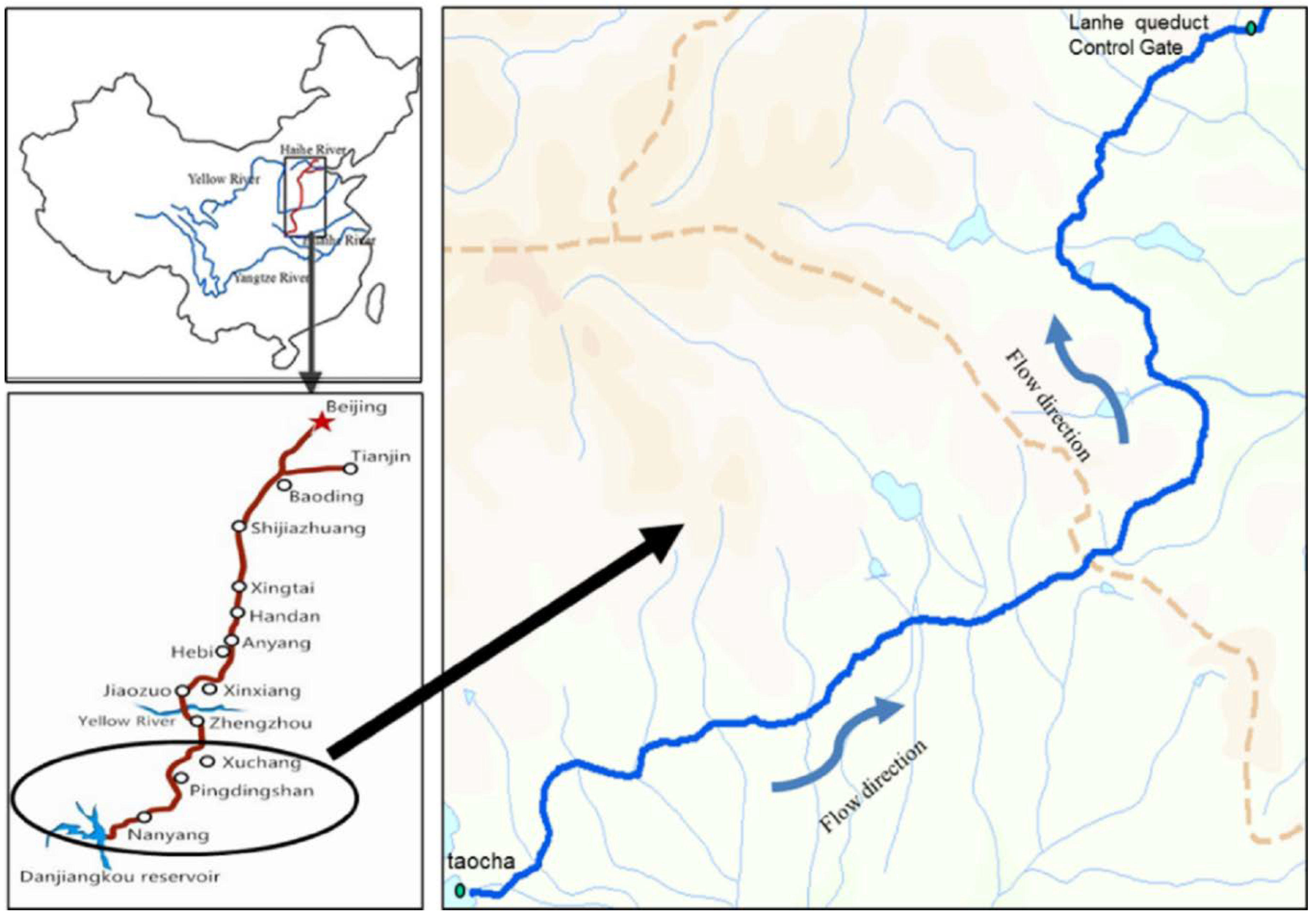
Along the main canal, areas with strong algae growth mainly appeared on both sides from the head of Taocha (Xichuan County, Nanyang City, Henan Province) to the control gate of the Lanhe Aqueduct (Jiaxian County, Pingdingshan City, Henan Province). This part of the main canal is approximately 304.55 km in length and accounts for 21.27% of the total length of the main canal. The areas with strong algae growth were all located in Henan Province, as shown in Figure 3. Algae were also present in other areas of the main canal, but the magnitude of their growth did not reach the level of disturbing the operation and management of the main canal.
Algae monitoring data for the main canal are extremely scarce. Because of the subtropical climate along the main canal, the temperature is generally more than 20 °C in the spring and summer, which is suitable for algae growth and reproduction. However, the spring results showed that the algae zones were not continuous and only grew on both sides of some canals or on one bank. Therefore, the factors influencing algae growth in the main canal needed to be analyzed from the viewpoint of hydrodynamics. Generally speaking, the water level and flow rate are the most basic and intuitive hydrodynamic parameters. For MRP, however, the water depth is basically stable at 4–6 m with little variation. Therefore, this study mainly focused on the influence of the flow rate on algae distribution.
2.2.2. Modeling Area
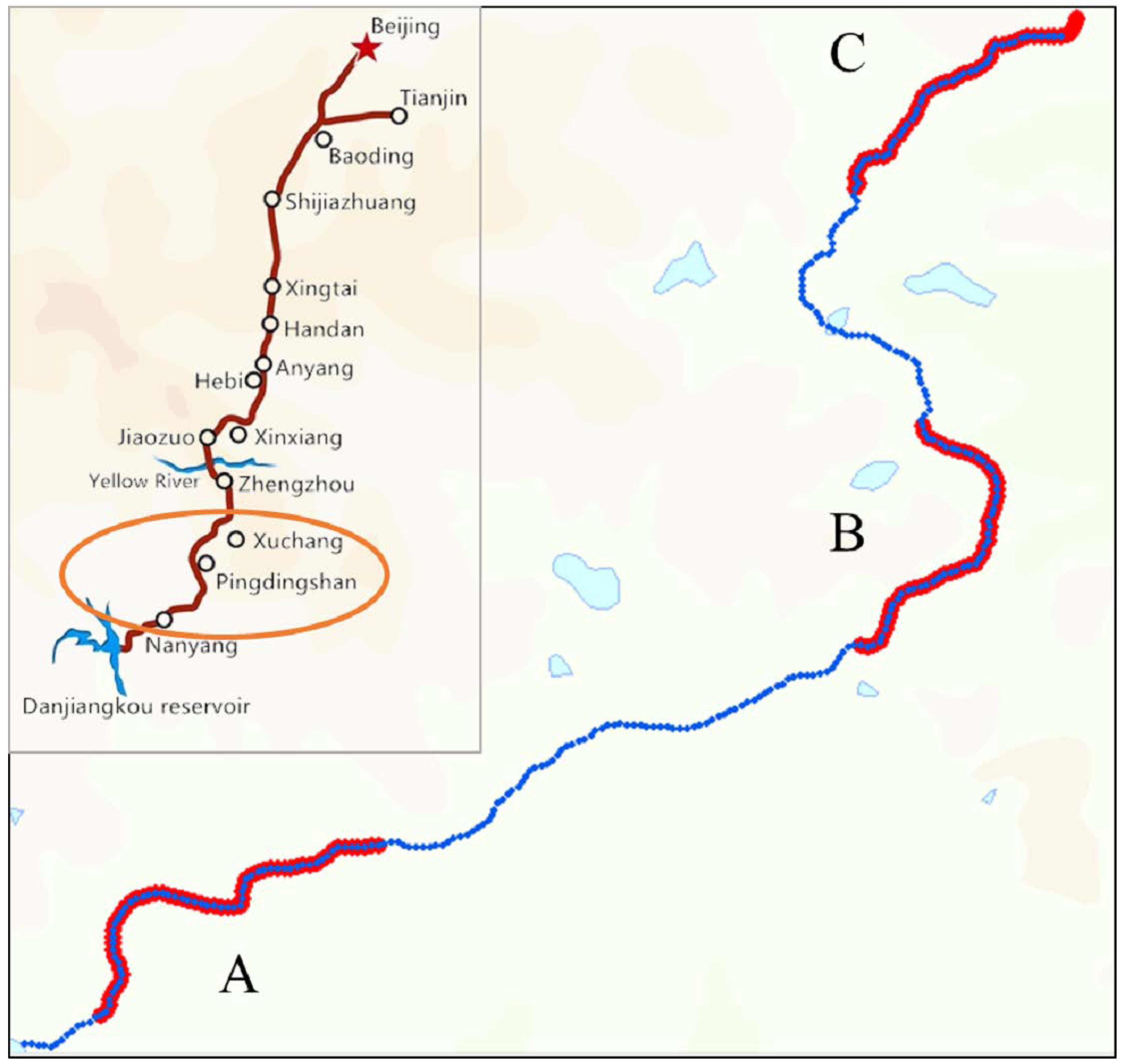
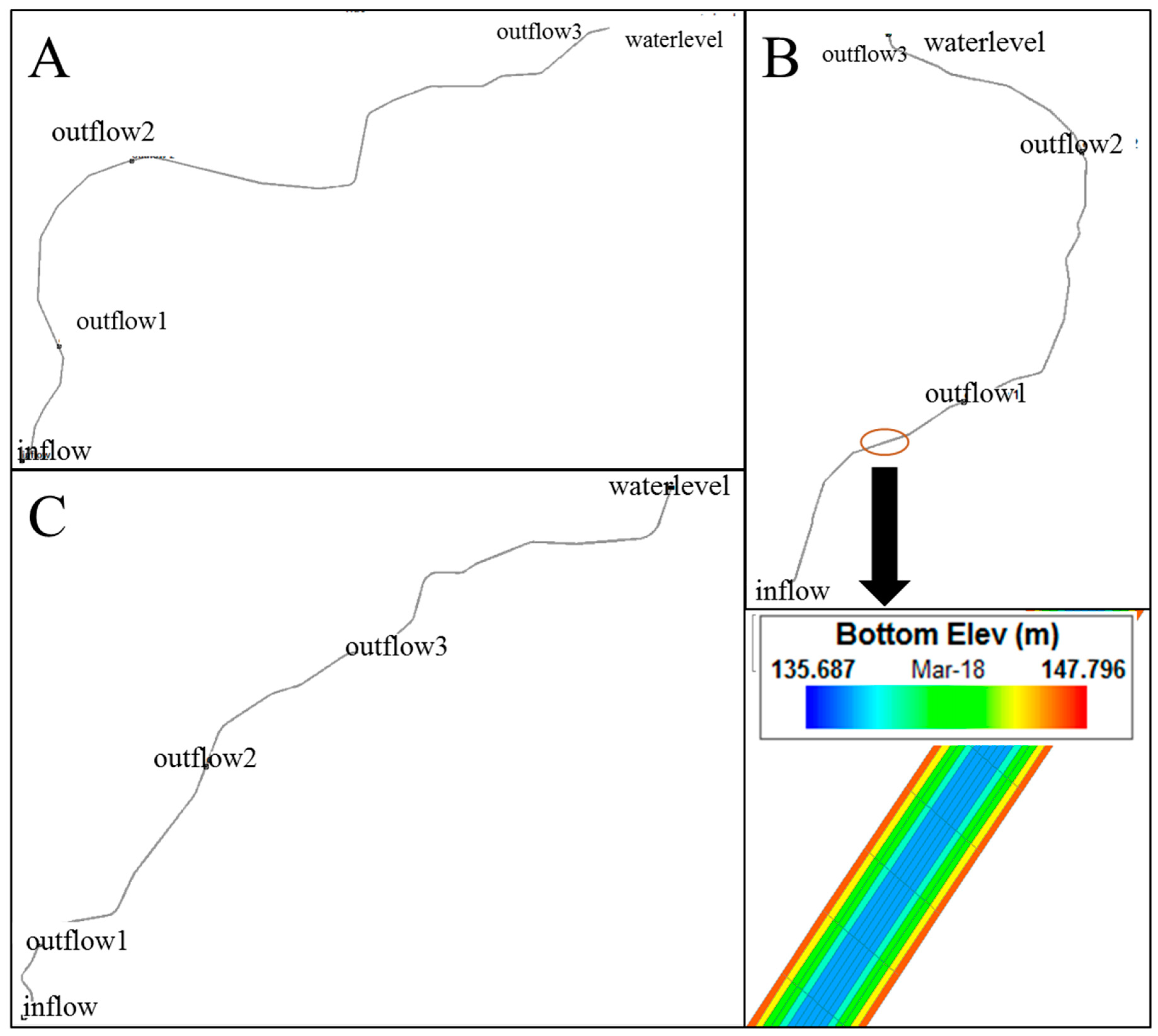
Figure 3 shows that the main canal sections with algae growth included the left bend near the head of the main canal, the relatively flat and straight section in Nanyang City, the right bend in Yexian County of Pingdingshan City, and the relatively flat straight section in Pingdingshan City. As shown in Figure 4, three representative sections were selected for modeling: (A) from the Diaohe Aqueduct Control Gate in Nanyang City, Xichuan County, to the Hebi Qihe Inverted Siphon Control Gate in Hebi City with a total length of 60.04 km; (B) from the Golden River Inverted Siphon Control Gate in Fangcheng County, Nanyang City, to the Lihe Aqueduct Control Gate in Yexian County, Pingdingshan City, with a total length of 49.54 km; and (C) from the Yinghe Inverted Siphon Control Gate in Baofeng County, Pingdingshan City, to the Yanyao Water Divide in Xuchang City, with a total length of 46.77 km.
The three selected sections were located at the left bend near the head of the main canal, the right bend section in Pingdingshan City, and the straight section in Pingdingshan City. They contained the basic characteristics of the main canal in areas with vigorous algae growth. The total canal length selected for modeling was 156.35 km, which accounted for 51.34% of the area with vigorous algae growth. The length of the algae growth zone selected for modeling was 45.77 km, which accounted for 62.60% of the total length of the zone. The algae zone length in Section A was 10.55 km, which accounted for 14.43% of the total algae zone length selected for modeling. The algae zone length on the left bank was 4.35 km, and that on the right bank was 6.20 km. The algae zone length in Section B was 15.09 km, which accounted for 20.64% of the total algae zone length selected for modeling. The algae zone length on the left bank was 7.97 km, and that on the right bank was 7.12 km. The algae zone length in Section C was 20.13 km, which accounted for 27.53% of the total algae zone length selected for modeling. The algae zone length on the left bank was 9.15 km, and that on the right bank was 10.98 km.
2.2.3. Modeling
The environmental fluid dynamic code (EFDC) model recommended by the United States Environmental Protection Agency [29] was used for the simulations. This is a comprehensive model developed by Hamrick of the Virginia Institute of Marine Science and is based on multiple mathematical models [30]. The EFDC model integrates modules for hydrodynamics, sediment transport, pollutant transport, and water quality prediction. It can be used to simulate one-, two-, and three-dimensional physical and chemical processes for water bodies including rivers, lakes, reservoirs, wetlands, and coastal waters [31,32]. At present, the EFDC model is one of the most widely used methods for simulating and predicting water environments both domestically and abroad [33]. Compared with other models, the EFDC model has better generality and powerful numerical calculation ability. It has a high computational efficiency, and it runs approximately 1.85 times faster than the Princeton ocean model (POM). The variable boundary processing technology is flexible, and the data output is widely used [34].
The physical processes and computational formats described by the EFDC model are consistent with the widely used Blumberg–Mellor model and Chesapeake Bay model of the American Engineering Corps. The EFDC model is based on a three-dimensional vertical hydrostatic assumption, the free surface problem, and turbulent mean motion equation for a variable-density fluid. The vertical coordinate is the sigma coordinate, and the plane is in Cartesian or curve orthogonal coordinates [35]. The turbulent kinetic energy, turbulent scale, temperature, and salinity equations are solved dynamically. The modified 2.5-order Mellor–Yamada closure model is used for the turbulence two-equation model. In addition, the EFDC model provides an optional bottom boundary layer submodel that can simulate the wave–current interaction in the boundary layer when the external high-frequency wave field is given. The EFDC model can solve the Eulerian transport and transformation equation of any number of dissolved and suspended phase materials simultaneously [36]. The EFDC model adopts the material conservation scheme, which can be used to simulate the dynamic changes of dry and wet grids in shallow-water areas [37]. The model provides a series of alternatives for simulating general flood control structures (e.g., weirs, spillways, and culverts). For simulations of the near-shore breaking zone, the EFDC model can consider the radiation stress from an external high-frequency surface gravity wave. The dissipation of external given waves due to breakage and bottom friction can also be added to the turbulent closure model in the form of a source term [38].
Boundary and Initial Conditions
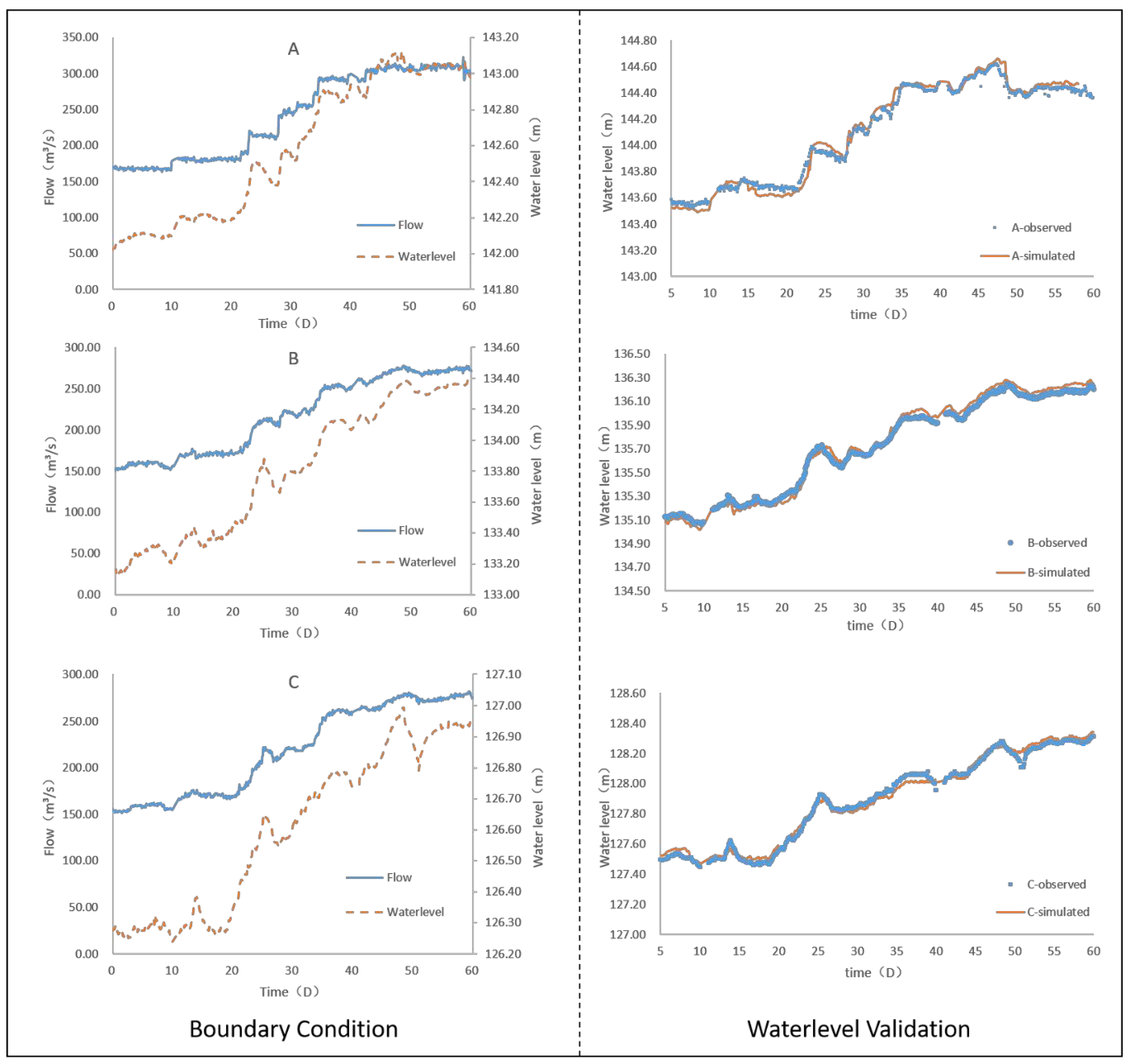
Initial conditions and boundary adjustments are necessary for solving the hydrodynamic equation of the EFDC model. The study area of the model is surrounded by specific boundaries, and the mathematical equations describe the various physical and chemical reactions of the water. To solve these equations, correct and reasonable initial and boundary conditions must be selected. The simulation time was set to 60 days, from 21 March to 20 May 2018, and the time step was 0.4 s. The measured data were used for the boundary conditions of the model. The discharge was used as the upper boundary, and the water level behind the sluice was used as the lower boundary, as shown in Figure 5. Section A had 14,880 grids, Section B had 14,925 grids, and Section C had 14,925 grids, as shown in Figure 6.
Model Verification
The EFDC model contains more than 130 parameters, so calibration is a key step for determining these parameters. Information on the parameter values was taken from technical reports, papers, manuals, and model reports on water bodies [39]. In many hydrodynamic models of rivers, estuaries, bays, and floodplains, the water level is often the preferred indicator for validation; there are far more cases where the water level was used for model validation than the flow rate [40]. During the simulation period, the water level in the main canal changed significantly. Figure 5 compares the simulated and measured water levels. The differences between the simulated and measured values were small with average and relative errors of 0.74 cm and 0.0051%, respectively, for Section A; 1.12 cm and 0.0086%, respectively, for Section B; and 0.96 cm and 0.0075%, respectively, for Section C.
3. Results and Discussion
In spring 2018, a field survey was conducted on the main canal. The statistical results showed that the total length of the algae growth zone in the middle line was approximately 73.12 km with a length of 35.79 km on the left bank and 37.33 km on the right bank. Based on the distribution of the algae zones, canal trend, and bending degree, the survey area was divided into three sections, as shown in Figure 7: A (A1, A2, A3), B (B1, B2, B3), and C (C1, C2, C3) The algae zone distribution regularities and hydrodynamic simulation results in the study area were analyzed separately, and the correlation between the algae zone growth length and flow rate distribution was analyzed. The results are given below.
3.1. Distribution Regularities of the Algae Zones
The investigation results for the algae zone distribution are presented below.
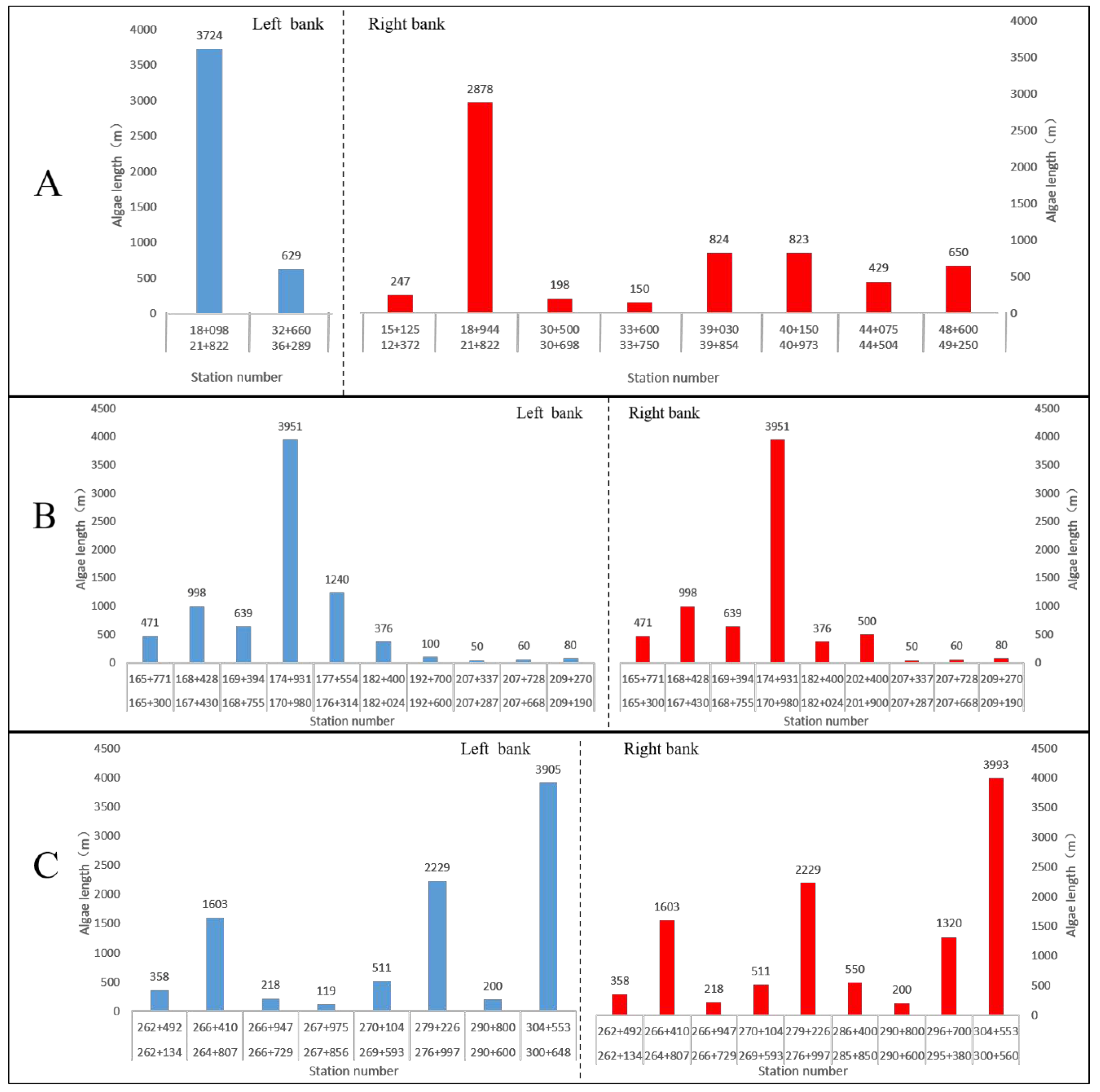
- The total canal length in Section A was 60.04 km. The engineering characteristics of the canal were as follows: a large bend with a length of approximately 15 km and an arc of approximately 60° (blue dotted circle in Figure 7; A2). There were 10 algae growth zones in Section A: two on the left bank and eight on the right bank. The length of each algae zone is shown in Figure 8. The longest algae growth zone on the left bank was 3724 m, and the longest algae zone on the right bank was 2878 m. As shown in Figure 7, the longest algae growth zones on the left and right banks were before the great bend of Section A (A1) (i.e., upstream of the blue dotted circle). The algae growth zone was concentrated in the great bend (A2), and there was almost no algae zone near the lower reaches of the greater bend (A3).
- The total canal length of Section B was 49.54 km. The engineering characteristics of the canal were as follows: a large curved section with a length of approximately 20 km and an arc of approximately 90° (orange dotted circle in Figure 7; B2). There were 19 algae growth zones in Section B: 10 on the left bank and nine on the right bank. The length of each algae zone is shown in Figure 8. The longest algae zone was 3951 m in length. The longest algae zones on the left and right banks were in front (B1) of the large bend section (i.e., upstream of the orange dotted circle). The algae zone in Section B was concentrated in the large bend, especially at the front and end (B1 and B2). From the number of algae zones, the section between B2 and B3 had a length of approximately 10 km with a curvature of approximately 120° and nine algae zones. The longest algae zone was still in front of the large curved section (B1), and only a few algae zones appeared in B3 after the large bend.
- The total canal length of Section C was 46.77 km. The section was characterized by a relatively small degree of bending overall. In contrast, there was a bending section with a large bending degree downstream of Section C (red dotted circle in Figure 7; C3). There were 17 algae growth zones in Section C: eight on the left bank and nine on the right bank. Figure 8 shows that the longest algae zone on the left bank was 3905 m, and the longest algae zone on the right bank was 3993 m. These zones were located at the same position in front of the large bend section (red virtual coil in Figure 7; C3).
Based on the algae distributions in Sections A–C, the following can be concluded:
- Large-scale algae zones often occurred at the front end of large curved sections in the canal. The largest algae zone appeared at the front of the large bends in Sections A and B (virtual coils in Figure 7). In Section C, although the overall bending degree was relatively small, there was a relatively large bend downstream of the section (virtual coil in Figure 7). The largest algae zone in Section C also appeared upstream of the bend.
- The algae zones were concentrated in curved sections. There were 64 curves with different bending degrees in the study area: 23 in Section A, 23 in Section B, and 18 in Section C. Among the positions with vigorous algae growth, seven in Section A were along bends, accounting for 30.44% of the total bend length and 70% of the total algae growth zones; nine in Section B were along bends, accounting for 39.13% of the total bend length and 81.82% of the total algae growth zones; and six in Section C, accounting for 33.33% of the total section length and 66.67% of the total number of algae growth zones.
3.2. Distribution Regularities of the Flow Rate
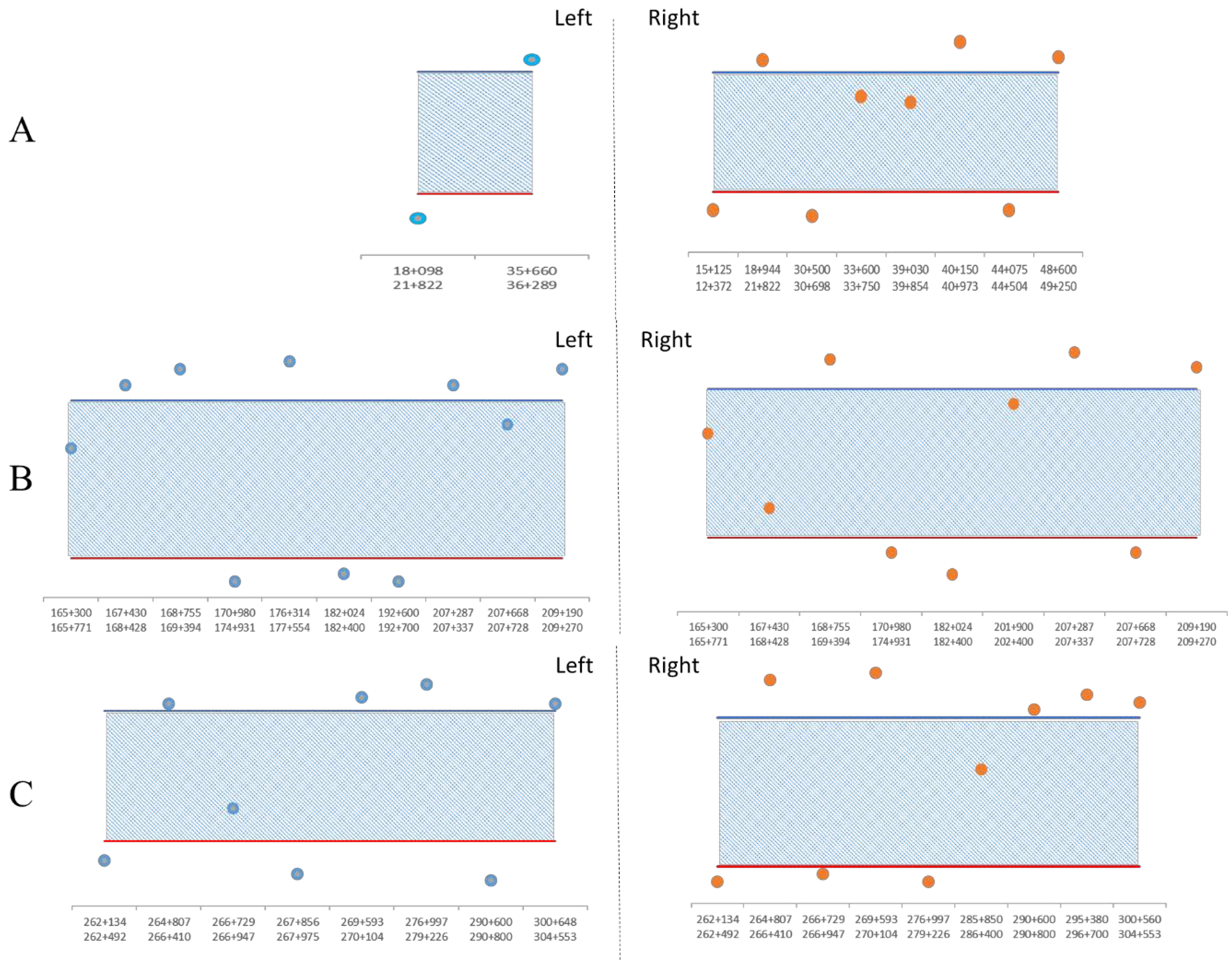
The simulation results of the hydrodynamic model were used to extract the positions of algae zones in Sections A–C and the average flow rates before and after the algae zones. The flow rates before, at, and after the algae zones were compared, as shown in Figure 9. For areas outside the shaded part, the average flow rate of the algae zone was less than the average flow rates before and after the zone. For the shaded part, the flow rate of the algae zone was not less than the average flow rates before and after the algae zone.
There were 46 algae zones in Sections A–C: 20 on the left bank and 26 on the right bank. Among them, 37 were outside the shaded area, accounting for 80.43% of the total algae zones: 17 on the left bank and 20 on the right bank. In Section A, eight algae zones had a flow rate less than that before and after, accounting for 80% of the total algae zones: the two on the left bank were both outside the shaded area, and two of those on the right bank were in the shaded area. In Section B, 14 algae zones had a flow rate less than those before and after, accounting for 77.78% of the total algae zones. Two algae zones on the left bank and three algae zones on the right bank had flow rates less than those before and after. In Section C, the flow rate of 15 algae zones was less than that before and after, accounting for 88.24% of the total algae zones. One algae zone on both sides of the bank had a flow rate less than those before and after.
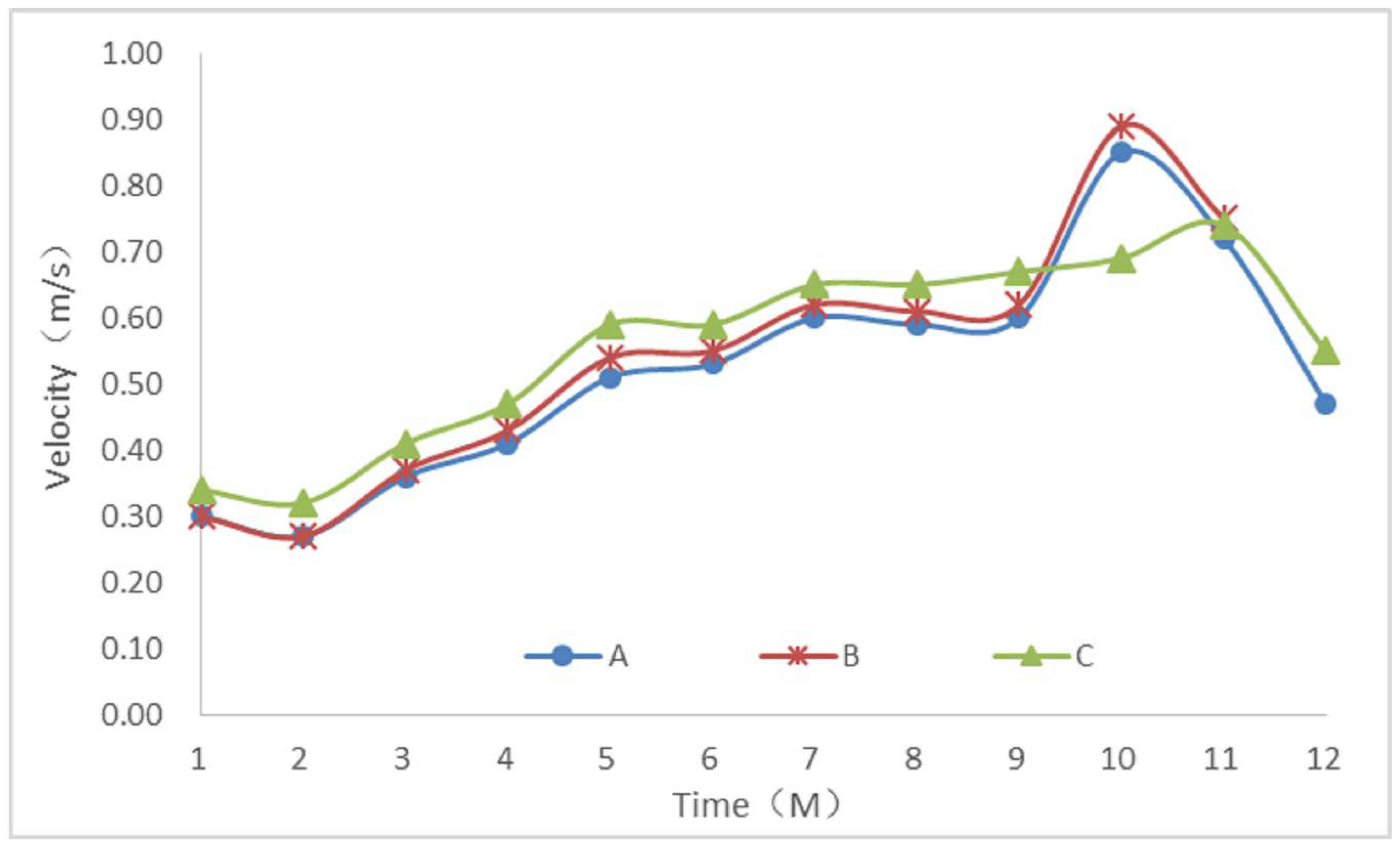
Figure 10 shows the measured flow rate data of Sections A–C for the whole year. The trends for the changes in flow rate were basically the same for each section. The maximum and minimum flow rates were respectively 0.85 and 0.27 m/s for Section A, 0.89 and 0.27 m/s for Section B, and 0.74 and 0.32 m/s for Section C. The minimum flow rates in the sections all occurred in February–March, and the maximum flow rates were in October–November. The range of the flow rate variation in the main canal was large, which indicated that the main canal had a large capacity and could operate safely in the case of large variations in the flow rate. This ensures that the hydrodynamic habitat conditions can be safely changed to suppress algae growth in the main canal.
3.3. Relationship between Algae and Flow Rate Distributions
Gray relational analysis (GRA) is a method of describing the strength and size of the relationship between factors by their gray relational degree. It involves analyzing and determining the contribution of factors to the main behavior by their gray relational degree. The relationship between factors is measured to give the degree of association. The basic concept involves studying the geometric correspondence between factors by using a mathematical method based on the data sequence of factors. That is, the closer the geometric shape is to a sequence curve, the greater the gray correlation degree between them, and vice versa. The essence of the GRA algorithm is that it provides a means of measuring the distance between two vectors. For the time factor, the vector can be regarded as being a time curve, with the GRA algorithm being used to measure whether the shapes and trends of the two curves are similar.
If the correlation degree is regarded as a distance between the measurement sequences, it can only be positive, but if it is regarded as being a measure of the correlation between sequences, it should be a number between −1 and 1. The commonly used gray relational measurement models, such as Deng’s relational degree, have a number of relational degrees between 0 and 1. As their values approach 1, the relationship between the evaluation object and the target becomes closer.
The length of the algae growth zone was selected as the parent factor, and the flow rate in the hydrodynamic habitat conditions affecting algae growth was selected as the subfactor. The calculation process is as follows:
- The parent factor is (), and the sub-factor is ().
- Dimensionless data processing.“Averaging” process:“Initialization” processing:where is the average of the observed values; is the k-th observed value; is the initial observed value.
- The correlation coefficients of the algae growth zone length and each index after the mean and initial values are calculated as follows:where is the correlation coefficient between the sub-factor and parent factor at time , is the absolute value of the difference between two sequences at time (), and are the maximum and minimum absolute values, respectively, of the time difference, and is the resolution coefficient. The resolution coefficient is an important factor that directly affects the resolution of the correlation analysis, and its value directly determines the distribution of the correlation coefficients. Different values greatly influence the rate of change in the correlation coefficient. The resolution coefficient is inversely proportional to the resolution. A smaller indicates a greater resolution. In many papers [41,42,43,44,45], ; for specific applications, .Based on , the following average values were obtained: and in Section A, and in Section B, and and in Section C. The following initial values were obtained: and in Section A, and in Section B, and and in Section C.
- Relevance Degree of the Parent Factor and Subfactor .The average relevance degree of a correlation coefficient is given bywhere is the degree of relevance.
Table 1 indicates that the correlation between the flow rate and length of the algae growth zone differs depending on whether the average or initial values were used for processing, but exceeded 0.55. When average values were used, the correlation degree exceeded 0.64, while the correlation degrees of Sections B and C was more than 0.75 with the initial value method.
According to the field investigation and model results, Table 2 shows the relationship between the length of the algae growth zone and the average flow rate in each canal section: a smaller average flow rate leads to a greater length of the algae growth zone.
Therefore, we can conclude that the flow rate in the main canal has a high degree of correlation with the length of the algae growth zone and thus has considerable influence.
4. Conclusions
Despite the emergence of algae in the main canal, there has been a lack of monitoring and research. Therefore, it is particularly important and urgent to investigate areas with vigorous algae growth to determine the source of the algae and analyze the key factors affecting the growth of algae in MRP. In this study, a field investigation, monitoring, and hydrodynamic simulation were used to analyze the differences between the hydrodynamic habitat conditions of areas with vigorous algae growth and other locations, establish the hydrodynamic habitat conditions of the main canal, and determine the growth, distribution, and correlation of macrobenthic algae in the main canal.
- The distribution of algae zones in Sections A–C showed that most algae zones occurred in curved sections, and the junction between straight and curved sections (i.e., the front of large bends) was most suitable for large algae zones to appear. Thus, to prevent and control algae in the main canal of the MRP, algae control devices should mainly be installed at the front of large bends with fewer devices at other positions. This will not only effectively prevent and control algae in the main canal, but also reduce the cost.The gray correlation method was used to calculate the correlation between the length of the algae growth zone and the flow rate. The results showed that the correlation between the length of the algae growth zone and the flow rate in Sections A–C was over 0.65 with the mean method and 0.55 with the initial value method. The correlation between Sections B and C was over 0.75, so the length of the algae zone is strongly correlated with the flow rate. According to the field investigation and model results, the relationship between the length of the algae growth zone and the average flow rate in each canal section: a smaller average flow rate leads to a greater length of the algae growth zone. Therefore, we come to the conclusion that the flow rate in the main canal has a high correlation with the length of the algae growth zone and thus a great influence.
- The flow rate at 80.43% of algae zones was less than those before and after the zones. Eight of these zones were in Section A, accounting for 80% of the total number of algae zones; 14 were in Section B, accounting for 77.78% of the total; and 15 were in Section C, accounting for 88.24% of the total. This shows that algae were more likely to grow and more algae zones appeared in areas with low flow rate.
- The historical flow rate data of the main canal showed that the flow rate varied widely. The maximum and minimum flow rates were respectively 0.85 and 0.27 m/s in Section A, 0.89 and 0.27 m/s in Section B, and 0.74 and 0.32 m/s in Section C. This indicates that the main canal has a large capacity to bear changes in the flow rate and can safely operate at high flow rates. This ensures that the hydrodynamic habitat conditions in the main canal can be safely changed to suppress algae growth.
- The change in the hydrodynamic conditions will lead to a change in the material transport in the water, which will affect the growth of algae. At the same time, hydrodynamic conditions will affect the attachment rate, attachment abundance, and biomass of Cladophora to some degree. At high flow rates, the close contact between the filaments of Cladophora can reduce the concentration of substances, both within the Cladophora and in the surrounding water, and the photosynthetic efficiency decreases due to the light-shielding effect, which is called the streamlining effect.Because the flow rate is the most basic and intuitive hydrodynamic parameter, this analysis of the relationship between the flow rate, algae growth, and distribution provides specific and effective suggestions for key prevention and control positions. It is suggested that the key prevention and control measures should be implemented at the large curved section of the main canal, at least at the front of the large curved section. This is clearly extremely important information for improving the efficiency of algae control in the main canal.
Author Contributions
J.Z. and J.Q. analyzed data formally, proposed the research, conducted fieldwork, and J.Z. drafted the original manuscript. X.Y. assisted J.Z. in data collection and research. X.L. supervised the overall research project, acquired funding to support this research.
Funding
This research was funded by the Major Science and Technology Program for Water Pollution Control and Treatment (2017ZX07108-001).
Acknowledgments
The anonymous reviewers and the editor will be thanked for providing insightful and detailed.
Conflicts of Interest
The authors declare no conflict of interest.
References
- Shen, H.; Cai, Q.; Zhang, M. Spatial gradient and seasonal variation of trophic status in a large water supply reservoir for the South-to-North Water Diversion Project, China. J. Freshw. Ecol. 2015, 30, 249–261. [Google Scholar] [CrossRef]
- Tang, C.H.; Yi, Y.J.; Yang, Z.F.; Cheng, X. Water pollution risk simulation and prediction in the main canal of the South-to-North Water Transfer Project. J. Hydrol. 2014, 519, 2111–2120. [Google Scholar] [CrossRef]
- Li, S.Y.; Li, J.Q.; Zhang, Q.F. Water quality assessment in the rivers along the water conveyance system of the Middle Route of the South to North Water Transfer Project (China) using multivariate statistical techniques and receptor modeling. J. Hazard. Mater. 2011, 195, 306–317. [Google Scholar] [CrossRef]
- Wang, P.L. Studies on the Formation Mechanism of Diatom Blooms in Hanjiang River from Hydrodynamics and Nutrition. Master’s Thesis, Huazhong Agricultural University, Wuhan, China, 2010. [Google Scholar]
- Zhang, W.H. Effects of Hydrodynamics on Nutrient Cycling and Algal Growth in Lake Tai. Master’s Thesis, Chinese Research Academy of Environmental Sciences, Beijing, China, 2017. [Google Scholar]
- Xu, L.; Feng, P.; Sun, D.M.; Li, F.W. Numerical simulation for the effect of temperature on the algae growth. J. Environ. Saf. 2013, 13, 76–81. [Google Scholar]
- Liu, F.L.; Jin, F. Control Effect of Current Velocity on Alga Growth in Eutrophication Water. Water Sav. Irrig. 2009, 9, 52–54. [Google Scholar]
- Jing, W.Q. Research on the Impact of Flow Velocity on the Eutrophicaton in Water Body. Master’s Thesis, Chongqing Jiaotong University, Chongqing, China, 2009. [Google Scholar]
- Gottlieb, A.D.; Richards, J.H.; Gaiser, E.E. Comparative study of periphyton community structure in long and short-hydroperiod Everglades marshes. Hydrobiologia 2006, 569, 195–207. [Google Scholar] [CrossRef]
- Havens, K.E.; Beaver, J.R.; Casamatta, D.A.; East, T.L.; James, R.T.; Mccormick, P.; Phlips, E.J.; Rodusky, A.J. Hurricane effects on the planktonic food web of a large subtropical lake. J. Plankton Res. 2011, 33, 1081–1094. [Google Scholar] [CrossRef] [Green Version]
- Raeder, U.; Ruzicka, J.; Goos, C. Characterization of the light attenuation by periphyton in lakes of different trophic state. Limnologica 2010, 40, 40–46. [Google Scholar] [CrossRef] [Green Version]
- Yan, R.R.; Png, Y.; Zhao, W.; Li, R.L.; Chao, J.Y. Influence of circumfluent type waters hydrodynamic on growth of algae. China Environ. Sci. 2008, 28, 813–817. [Google Scholar]
- Zhang, Y.M.; Zhang, Y.C.; Zhang, L.J.; Gao, Y.X. The influence of lake hydrodynamics on blue algal growth. China Environ. Sci. 2007, 27, 707–711. [Google Scholar]
- Wang, J.H. The Experimental Study on the Influences of Flow Velocity on Algae Growth. Master’s Thesis, Tsinghua University, Beijing, China, 2012. [Google Scholar]
- Wu, X.H.; Li, Q.H. Reviews of influences from hydrodynamic conditions on algae. Ecol. Environ. Sci. 2010, 19, 1732–1738. [Google Scholar]
- Jiao, S.J. The Effects of Velocity of Glow to the Growth of Algae in Low Current Area of the Three Gorges. Master’s Thesis, Southwest University, Chongqing, China, 2007. [Google Scholar]
- Hondzo, M.M.; Kapur, A.; Lembi, C.A. The effect of small-scale fluid motion on the green alga. Hydrobiologia 1997, 364, 225–235. [Google Scholar] [CrossRef]
- Ding, L.; Zhi, C.Y. Environmental effects on diatom and its monitor of environment. J. Guizhou Norm. Univ. (Nat. Sci.) 2006, 24, 13–16. [Google Scholar]
- Yu, L.H.; Guo, Y.Q. Influence of Dynamic Condition to the Algae of the Reservoir by Diverting the Yellow River. Yellow River 2011, 81–82. [Google Scholar]
- Wang, H.P.; Xia, J.; Xie, P.; Dou, M. Mechanisms for hydrological factors causing algal blooms in Hanjiang River—Based on kinetics of algae growth. Resour. Environ. Yangtze Basin 2004, 13, 282–285. [Google Scholar]
- Li, J.X.; Du, B.; Sun, Y.S. Effcet of hydrodynamics on the eutrophication. Water Resour. Hydropower Eng. 2005, 5, 15–18. [Google Scholar]
- Huang, C.; Zhong, C.H.; Deng, C.G.; Xing, Z.G. Preliminary study on correlation between flow velocity and algae along Daning River’s backwater region at sluice initial stages in the Three Gorges Reservoir. J. Agro-Environ. Sic. 2006, 25, 453–457. [Google Scholar]
- Borchardt, M.A. Effects of flowing water on nitrogen-limited and phosphorus-limiter photosynthesis and optimum N/P ratios by Spirogyra-Fluviatilis (Charophyceae). J. Phycol. 1994, 30, 418–430. [Google Scholar] [CrossRef]
- Healey, F.P. Interacting effects of light and nutrient limitation on the growth rate of Synechococcus linearis (Cyanophyceae). J. Phycol. 2010, 21, 134–146. [Google Scholar] [CrossRef]
- Pannard, A.; Bormans, M.; Lagadeuc, Y. Short-term variability in physical forcing in temperate reservoirs: Effects on phytoplankton dynamics and sedimentary fluxes. Freshw. Biol. 2007, 52, 12–27. [Google Scholar] [CrossRef]
- Huisman, J.; Sharples, J.; Stroom, J.M.; Visser, P.M.; Kardinaal, W.E.A.; Jolanda, M.H.V.; Sommeijer, B. Changes in turbulent mixing shift competition for light between phytoplankton species. Ecology 2004, 85, 2960–2970. [Google Scholar] [CrossRef]
- Zhu, J.; Lei, X.H.; Zheng, H.Z. Risk analysis and emergency countermeasures for oil pollution in main channel of South to North Water Transfer Project. In Proceedings of the 1st International Symposium on Water System Operations, ISWSO 2018, Beijing, China, 16–20 October 2018. [Google Scholar]
- Liu, X.; Chen, Y.W. A review on the ecology of Cladophora. J. Lake Sci. 2018, 30, 19–34. [Google Scholar]
- Zhang, H. Simulation Study on Water Environment of Dianchi Based on the EFDC. Master’s Thesis, Zhejiang University, Hangzhou, China, 2017. [Google Scholar]
- Wu, G.Z.; Xu, Z.X. Prediction of algal blooming using EFDC model: Case study in the Daoxiang Lake. Ecol. Model. 2011, 222, 1245–1252. [Google Scholar] [CrossRef]
- Tang, T.J.; Yang, S.; Yin, K.H. Simulation of eutrophication in Shenzhen Reservoir based on EFDC model. J. Lake Sci. 2014, 26, 393–400. [Google Scholar] [Green Version]
- Gong, R.; He, Y.; Xu, L.G.; Wang, D.G. The application progress of environmental fluid dynamics code (EFDC) in lake and reservoir environment. Trans. Oceanol. Limnol. 2016, 6, 12–19. [Google Scholar]
- Ding, Y.; Jia, H.F.; Ding, Y.W.; Sun, Z.X. Hydrodynamic optimization of urban river network of water towns based on EFDC model. Acta Sci. Circumst. 2016, 36, 1440–1446. [Google Scholar]
- Liu, W.C.; Kuo, J.T. Evaluation of marine outfall with three-dimensional hydrodynamic and water quality modeling. Environ. Model. Assess. 2007, 12, 201–211. [Google Scholar] [CrossRef]
- Zang, Y.F.; Wang, Y.L.; Wang, L. Overview and application analysis of EFDC model. Environ. Impact Assess. 2015, 37, 70–72. [Google Scholar]
- Duan, Y. Water Environment Dynamics Simulation Technology Research Based on EFDC—DanJiangKou Reservoir as an Example. Master’s Thesis, China University of Geosciences, Wuhan, China, 2014. [Google Scholar]
- Zhou, X.B.; Wu, J.; Zhang, Z.Y.; Zhuang, W. Application study of EFDC on division of drinking water source conservation area by taking one drinking water plant in Hangjiahu region as a case. Environ. Sci. Surv. 2009, 28, 30–32. [Google Scholar]
- Chen, H.Y. Study on Water Quality Early Warning of Huainan Water Source Based on EFDC Model. Master’s Thesis, Minzu University of China, Beijing, China, 2012. [Google Scholar]
- Zhen, G.J. Hydrodynamics and Water Quality: Modeling Rivers, Lakes, and Estuaries; Wiley-Interscience: Hoboken, NJ, USA, 2008. [Google Scholar]
- Liu, X.M.; Li, J.Q.; Dou, X.M.; Wang, Y.L. The Application and Advance of Environmental Fluid Dynamics Code (EFDC) in Estuarine Water Environment. Environ. Sci. Technol. 2011, 34, 136–140. [Google Scholar]
- Satapathy, B.K.; Bijwe, J.; Kolluri, D.K. Assessment of fiber contribution to friction material performance using gray relational analysis (GRA). J. Compos. Mater. 2005, 40, 483–501. [Google Scholar] [CrossRef]
- Sun, Y.G. Research on Gray Relational Analysis and Its Application. Master’s Thesis, Nanjing University of Aeronautics and Astronautics, Nanjing, China, 2007. [Google Scholar]
- Wang, J.M.; Guo, J.W.; Lian, X.J. Comparative study on two improved Gray Relational Analysis. J. North China Electr. Power Univ. 2005, 6, 72–76. [Google Scholar]
- Deng, J.L. Gray System Theory Tutorial; Huazhong University of Technology Press: Wuhan, China, 1990. [Google Scholar]
- Shi, S.L. Theory analysis of interzone of resolution ratio ρ in gray interrelated modeland practical validation in safety valuation of working faces. J. Xiangtan Min. Inst. 1999, 2, 7–11. [Google Scholar]
Figure 1.
Algae in the main canal of the Middle Route of the South-to-North Water Diversion Project (MRP).
Figure 1.
Algae in the main canal of the Middle Route of the South-to-North Water Diversion Project (MRP).

Figure 2.
Algae capture.

Figure 3.
Field investigation area.

Figure 4.
Modeling scope.

Figure 5.
Boundary conditions and model validation.

Figure 6.
Mesh generation.

Figure 7.
Distribution of algae growth zones.

Figure 8.
Lengths of algae growth zones.

Figure 9.
Simulated flow rate results.

Figure 10.
Historical measured flow rate (M—month).


Table 1.
Relevance table.
| Index | Flow Rate (m/s) | Flow Rate (m/s) | Flow Rate (m/s) |
|---|---|---|---|
| Average | 0.656 | 0.742 | 0.648 |
| Initialization | 0.555 | 0.772 | 0.758 |
Table 2.
Length of the algae growth zone and average flow rate.
| Index | Section A | Section B | Section C |
|---|---|---|---|
| Length of algae growth zone (km) | 10.55 | 15.09 | 20.125 |
| Ratio of length of algae growth zone to length of canal section (%) | 17.58 | 30.46 | 43.03 |
| Average flow rate (m/s) | 0.314 | 0.239 | 0.225 |
© 2019 by the authors. Licensee MDPI, Basel, Switzerland. This article is an open access article distributed under the terms and conditions of the Creative Commons Attribution (CC BY) license (http://creativecommons.org/licenses/by/4.0/).
Share and Cite
MDPI and ACS Style
Zhu, J.; Lei, X.; Quan, J.; Yue, X. Algae Growth Distribution and Key Prevention and Control Positions for the Middle Route of the South-to-North Water Diversion Project. Water 2019, 11, 1851. https://doi.org/10.3390/w11091851
AMA Style
Zhu J, Lei X, Quan J, Yue X. Algae Growth Distribution and Key Prevention and Control Positions for the Middle Route of the South-to-North Water Diversion Project. Water. 2019; 11(9):1851. https://doi.org/10.3390/w11091851
Chicago/Turabian StyleZhu, Jie, Xiaohui Lei, Jin Quan, and Xia Yue. 2019. "Algae Growth Distribution and Key Prevention and Control Positions for the Middle Route of the South-to-North Water Diversion Project" Water 11, no. 9: 1851. https://doi.org/10.3390/w11091851
Note that from the first issue of 2016, this journal uses article numbers instead of page numbers. See further details here.