On Some Properties of the Glacial Isostatic Adjustment Fingerprints


1
Dipartimento di Scienze Pure e Applicate (DiSPeA), Sezione di Fisica, Università degli Studi di Urbino “Carlo Bo”, I-61029 Urbino, Italy
2
Istituto Nazionale di Geofisica e Vulcanologia (INGV), Via di Vigna Murata 605, I-00143 Rome, Italy
*
Author to whom correspondence should be addressed.
†
These authors contributed equally to this work.
Water 2019, 11(9), 1844; https://doi.org/10.3390/w11091844
Submission received: 31 July 2019
/
Revised: 28 August 2019
/
Accepted: 2 September 2019
/
Published: 5 September 2019
(This article belongs to the Special Issue Past, Present and Future Trends in Sea Level Change)
Abstract
:Along with density and mass variations of the oceans driven by global warming, Glacial Isostatic Adjustment (GIA) in response to the last deglaciation still contributes significantly to present-day sea-level change. Indeed, in order to reveal the impacts of climate change, long term observations at tide gauges and recent absolute altimetry data need to be decontaminated from the effects of GIA. This is now accomplished by means of global models constrained by the observed evolution of the paleo-shorelines since the Last Glacial Maximum, which account for the complex interactions between the solid Earth, the cryosphere and the oceans. In the recent literature, past and present-day effects of GIA have been often expressed in terms of fingerprints describing the spatial variations of several geodetic quantities like crustal deformation, the harmonic components of the Earth’s gravity field, relative and absolute sea level. However, since it is driven by the delayed readjustment occurring within the viscous mantle, GIA shall taint the pattern of sea-level variability also during the forthcoming centuries. The shapes of the GIA fingerprints reflect inextricable deformational, gravitational, and rotational interactions occurring within the Earth system. Using up-to-date numerical modeling tools, our purpose is to revisit and to explore some of the physical and geometrical features of the fingerprints, their symmetries and intercorrelations, also illustrating how they stem from the fundamental equation that governs GIA, i.e., the Sea Level Equation.
1. Introduction
Since the Glacial Isostatic Adjustment (GIA) caused by the melting of past ice sheets is still contributing to present-day regional and global sea-level variations, understanding its spatio-temporal variability is important to interpret the effects of present climate change. However, because GIA is also affecting the shape of the Earth and its gravity field, it has a clearly established role in the interpretation of a wide range of geophysical data, obtained by means of ground-based or space-borne geodetic observations. The relevance of GIA modeling in various fields of the Geosciences and its increasing role in the framework of global change constitutes the motivation of this study, mainly aimed at reviewing systematically the imprints of GIA and to describe their geometry in connection with the Sea Level Equation (SLE).
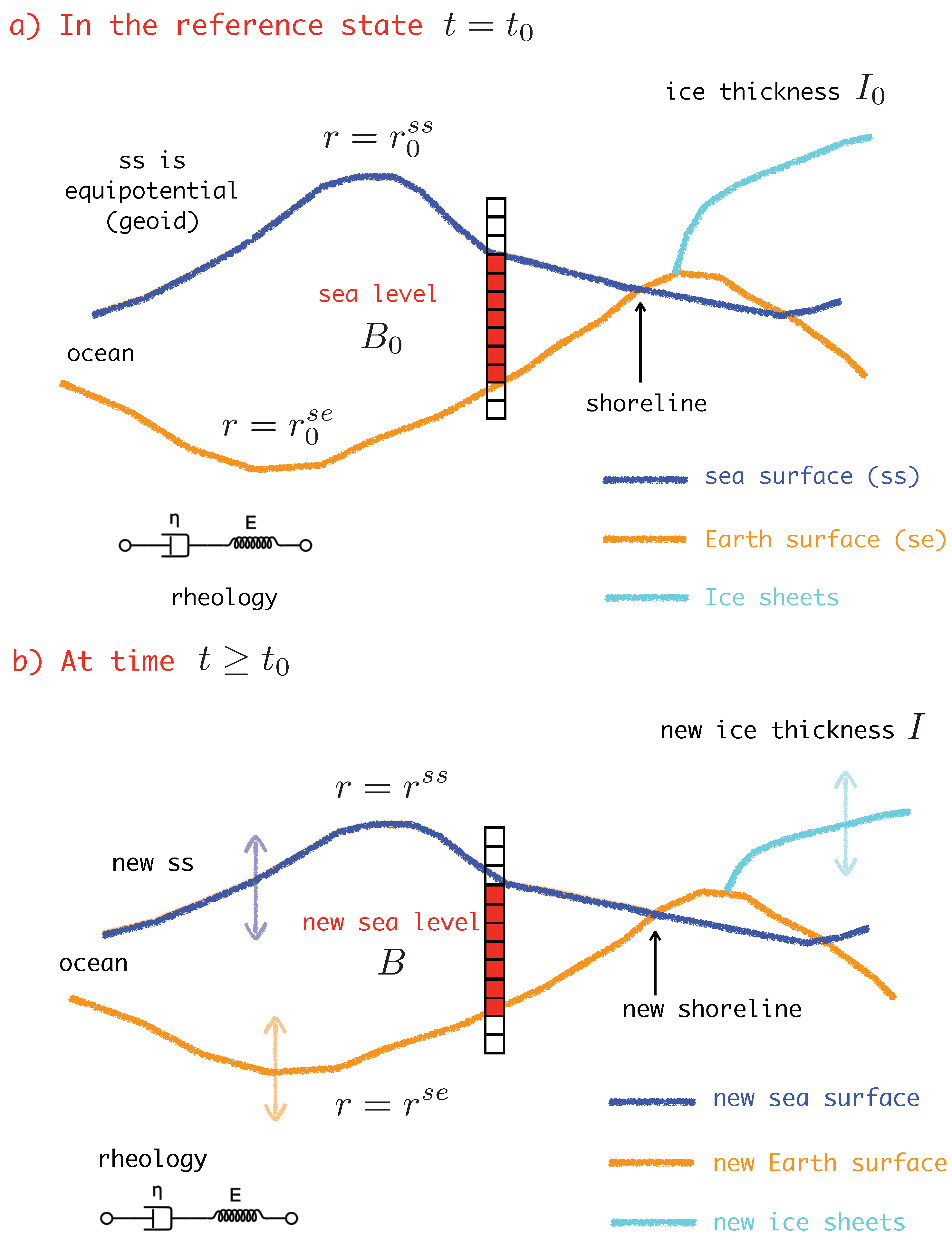
To introduce GIA, it is convenient to define a reference state in which the solid Earth, the ice sheets and the oceans are in an equilibrium configuration, sketched in Figure 1a, and to compare it to a subsequent perturbed state. This approach was originally proposed by Farrell and Clark [1], hereafter referred to as FC76, in their seminal work where the SLE was introduced first. The reference configuration can be chosen arbitrarily, but for our discussion it is convenient to refer to the Last Glacial Maximum (LGM, ∼21,000 years ago). The load acting on the Earth’s surface in the reference state (i.e., the mass per unit area) is and is the ice thickness, with where is colatitude and is longitude. The SLE has can be employed to predict how sea level shall change at an arbitrary location , when the configuration of the system portrayed in Figure 1a evolves in a new state shown in Figure 1b at time , in which the surface load and the ice thickness are and , respectively. Despite the global variations observed in the new state, (i) the mass of the system (ice+oceans+solid Earth) must be conserved, and (ii) the new sea surface must remain an equipotential; ultimately, these are the two fundamental principles that the SLE makes manifest.
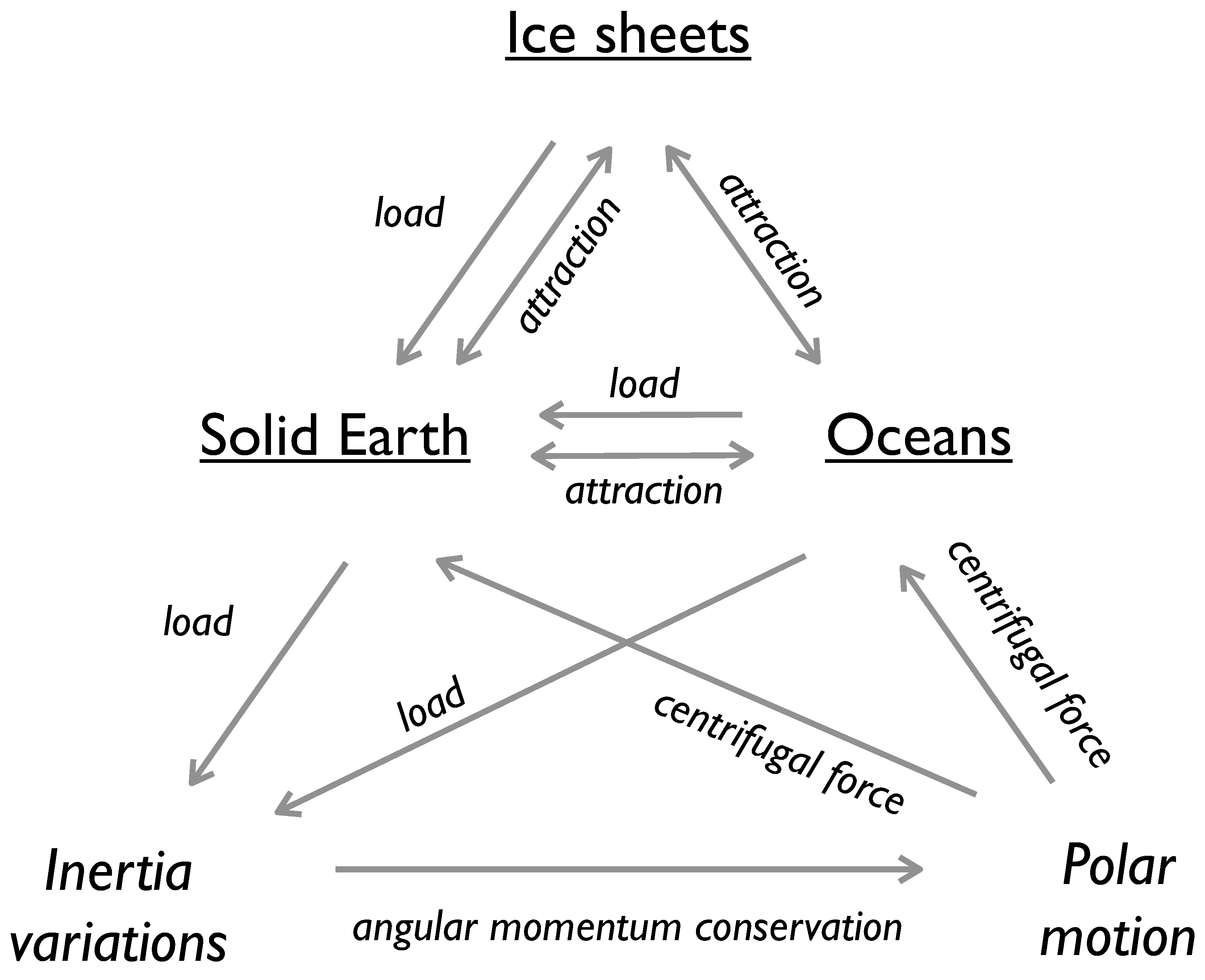
The interactions responsible for the changes observed in the new state are qualitatively sketched in the diagram of Figure 2, freely modified from Clark et al. [2]. Since the interactions are operating simultaneously and at all spatial scales, their contributions cannot be easily disentangled, which makes the interpretation of the GIA effects on sea level and on various geodetic quantities particularly challenging. In the top part, the figure is showing the three fundamental elements of the SLE, i.e., the ice sheets, the solid Earth, and the oceans [3]. As indicated by the arrows, these elements are interacting by two mechanisms: (i) surface loading and (ii) mutual gravitational attraction.
The waxing and waning ice sheets, by changing the local ice masses, exert a load at the surface of the solid Earth (ice loading, related to glacio-isostasy), but the mass variation of the oceans is also loading the Earth, acting on the seafloor (water loading, associated to hydro-isostasy). These two non-uniform loads are tightly interconnected, since the mass conservation of the system (water + ice) imposes that, on average, the load variation vanishes across the Earth’s surface. Due to the mantle imperfect elasticity, the past loads also induce delayed and still persistent effects that are manifest as a global state of isostatic disequilibrium. Furthermore, the equipotential surfaces of the Earth’s gravity field are twisted by the mass redistributed over the solid Earth and in the oceans, causing variations of the geoid. The three elements that enter into the SLE are all affected by gravitational attraction. In particular, the sea surface is warped by the attraction of the continental ice sheets, but at the same time the geoid variations caused by the solid Earth deformation modify the shape of the oceans. The bottom part of Figure 2 considers further interactions driven by the Earth’s irregular rotation. Inertia perturbations, associated to long wavelength deformations and sea-level variations of harmonic degree , drive excursions of the rotation axis in order to conserve the Earth’s angular momentum [4]. The consequent variation of the centrifugal potential alters, in turn, both the solid Earth and the sea surface, a process that is known as rotational feedback on sea level, see Peltier [5].
The inextricably related interactions first acknowledged by Clark et al. [2] and illustrated in Figure 2 are responsible for the regional imprints of GIA. As first noted by Woodward [6] and later discussed by Daly [7], Walcott [8] and Farrell and Clark [1], the sea-level variations associated with glacial isostasy depart significantly from the spatially uniform pattern that we would observe for a rigid, non-gravitating and non-rotating Earth (i.e., ignoring the interactions). Often, in the geological literature the spatially uniform sea-level change is referred to as eustatic, a word attributed to Suess [9]; eustatic variations only depend on the history of the past grounded ice volume [10]. Presently, the term barystatic is preferred [11]. The interactions are responsible for a global pattern of relative sea level (RSL) variations during the melting of the late-Pleistocene ice sheets, which Clark et al. [2] have characterized by defining six RSL zones, labelled from I to (see their Figure 5); within each zone, the sea-level signatures are similar to one another. The RSL zones encompass the glaciated areas (zone I), the region of the collapsing fore-bulge (), the time-dependent emergence () and the oceanic submergence zone (), the oceanic emergence region (V), and the continental shorelines (). Subsequently, Mitrovica and Milne [12] have studied the nature of the RSL zones in connection with the various terms of the SLE, describing the physical mechanisms responsible for their establishment and unveiling the processes of continental levering and ocean siphoning. Following the above studies, the spatial variability in sea level associated with GIA has been widely investigated with the aim of reconstructing the history of deglaciation since the LGM (see e.g., [13,14,15]). On a more limited spatial scale, the concept of RSL zone has also been useful to interpret the Holocene sea-level variations across the Mediterranean Sea [16,17].
The study of paleo-shorelines has allowed to define the broad features of the pattern of RSL zones since the LGM (see, e.g., Lambeck and Chappell [18]). However, the present-day trends of sea level detected at tide gauges or by satellite altimetry should be certainly also affected by contemporary variations in the state of the cryosphere driven by global warming. In this context, the question has not been addressed until the work of Plag and Jüettner [19], who have first coined the term of fingerprint (function). Quoting their same words, …The elastic response of the Earth to present-day changes in the cryosphere can be expected to produce a similar fingerprint, which should be present in the tide gauge data. Based on these fingerprints, tide gauge trends, in principle, can be inverted for ice load changes [19]. However, after having analyzed the relative sea-level trend for some long tide gauge time series, Douglas [20] concluded that unambiguous evidence for fingerprints of glacial melting was not found, most likely due to the presence of other signals present in sea-level records that cannot easily be distinguished. Recently, Spada and Galassi [21] have quantitatively compared the harmonic power spectrum of contemporary sea-level change to that of GIA, including the contribution due to the disintegration of the past ice sheets and that associated to present deglaciation. They have shown that the power of GIA from past ice melting is comparatively modest at all harmonic degrees, with the possible exception of harmonic degree , and it cannot emerge from the steric component that dominates current sea-level rise [22]. Notwithstanding the difficulty of visualization, the concept of sea-level fingerprint has undoubtedly gained an important role in the interpretation of the trends of contemporary [23,24,25,26,27] and future sea-level rise [28,29,30].
In this work, we aim at exploring and reviewing the properties and the symmetries of the GIA fingerprints presently associated with the melting of past ice sheets, as well as the intercorrelations among them. Much of what we present in this paper can be also applied to the fingerprints of present ice melting, which obey the SLE as well; these have been discussed in various places, see e.g., [31] and references therein. Although we are aware that uncertainties on the Earth’s viscosity profile and the chronology of deglaciation affect significantly the pattern and the amplitude of the GIA fingerprints [32], here for simplicity we shall only consider a specific GIA model, leaving an error analysis to future work, along the lines of Melini and Spada [32]. The paper is organized as follows. In Section 2 we review the theory behind the SLE. In Section 3 we briefly present the GIA model used and the numerical approach adopted. In Section 4 we illustrate some of the properties of the present-day GIA fingerprints associated with the melting of the past ice sheets, which in Section 5 are exploited to interpret the global uplift pattern of continents currently detected by GPS data. Our conclusions are drawn in Section 6.
2. Theory
Here we briefly introduce the essentials of the SLE theory, necessary to illustrate the geometry of the GIA fingerprints in Section 4 below. The reader is referred to Spada and Melini [33] (hereinafter SM19) and to its supplement for a more detailed and self-contained presentation. The paper SM19 and its supplement are presently (August 2019) submitted to Geoscientific Model Development (GMD), the interactive open-access journal of the European Geosciences Union at https://www.geosci-model-dev-discuss.net/gmd-2019-183/. The open-source program SELEN (SELEN version 4.0) can be obtained from https://zenodo.org/record/3377404. We note that the SLE theory does not account for tectonic deformations nor for variations in the temperature or salinity of the ocean water, which we do not consider in our analysis.
In the reference state considered in Figure 1a, sea level is defined by the difference
where are the coordinates of a given point on the Earth’s surface, while and are the radii of the (equipotential) sea surface and of the solid Earth in a geocentric reference frame with origin in the whole-Earth center of mass, respectively. As shown in Figure 1a, would be directly measured by a stick meter, i.e., a tide gauge, placed at . Assuming that the horizontal displacement of the stick-meter has been negligible in comparison to vertical displacement, in the new state sea level is
where and denote the new radius of the equipotential sea surface and of the solid surface of the Earth, respectively. Note that topography is related to sea level through
Combining (2) with (1), relative sea-level change
can be also expressed as
where
is the sea surface variation, or absolute sea-level change, and
is the vertical displacement of the Earth’s surface. Equation (5) represents the most basic form of the SLE. We note that, being defined as a double difference, relative sea-level change is not dependent upon the choice of the origin of the reference frame, i.e., it is an absolute quantity. Quantities and , however, depend on the choice of the origin.
The sea surface variation is tightly associated to the variation of the geoid height. However, as remarked by FC76, is not the variation of the geoid height: i.e., on a rigid Earth model, there is no distinction between changes in geoid radius and changes in sea level, but it is important to realize the difference between these quantities for deformable Earth models [1]. A further problem arises from the fact that, in the new state, the volume of the oceans is varied to compensate the mass lost or gained by the continental ice sheets. Indeed, as pointed out by Tamisiea [34], some confusion arose recently about the definition of , which sometimes is still used as a synonymous of geoid height variation; the confusion is attributed to often inconsistent terminology between various disciplines. FC76 have shown that the sea surface height variation is
where
is the variation of the geoid radius relative to the reference state, is the variation of the total gravity potential of the Earth system, taking both surface loading and rotational contributions into account, g is the reference surface gravity acceleration and c is a yet undetermined spatially invariant term, notorious within the GIA community as the FC76 c-constant. In the following, Equation (8) shall be referred to as FC76 formula. Thus, using Equation (8) in (5), the SLE reads
where we have defined the sea-level response function as the difference
It is now convenient to average both sides of Equation (10) over the oceans, where the ocean-average of any function is defined, at time t, as
where denotes the integral over the time-dependent surface of the oceans, is their area at time t, is the element of area over the surface of the sphere, and a the average Earth’s radius. We recall that the surface of the oceans is the region where , where O is the ocean function (OF) defined as
where and are the densities of ice and water, respectively. For , the ocean is ice-free, or there is floating ice; for , the ice is grounded either below or above sea level, or the land is ice-free. Using a continent function defined as is sometimes useful. Since , solving Equation (10) with respect to the FC76 constant gives
where we have defined . Hence, using Equation (14) into (10), the SLE is further transformed into
The response function embodies all the interactions qualitatively described in Figure 2; following SM19, we split it into a contribution due to surface loads and gravitational attraction (labeled by sur) and one due to rotational effects (rot), with
where and . According to Farrell [35], is given by a 3-D spatio-temporal convolution that involves the surface Green’s function for sea level and the surface load variation , where L and denote the surface load in an arbitrary state and in the reference state, respectively, and
while following Milne and Mitrovica [36], can expressed as a 1-D time convolution between the rotation Green’s function for sea level and the centrifugal potential variation, with
where () are the spherical harmonic degree and order, respectively (with and ). Han and Wahr [37] and Milne and Mitrovica [36], however, have shown that is essentially a spherical harmonic function of degree and order . The Green’s functions and are expressed by particular combinations of loading Love numbers and tidal Love numbers, respectively. It is important to note that the harmonic coefficients of , i.e., , depend linearly from those of the surface load variation (see supplement of SM19 for details).
An explicit expression for in Equation (15) is obtained applying the mass conservation principle that according to SM19 can be stated in various equivalent ways. Here it is convenient to use the form
where the average over the whole Earth’s surface is defined, in analogy with Equation (12), as . We refer to mass conserving loads that obey Equation (19) as physically plausible loads. As shown in SM19, condition (19) is equivalent to
where is the spherical harmonic component of the surface load for degree and order . Using the result
(SM19) and some algebra, from the constraint of mass conservation we obtain
where (equivalent sea-level change) is defined as
with denoting the time variation of the grounded ice mass, and term
is associated with ocean function variations, where and are the initial topography and the initial OF, respectively. We note that in the fixed-shorelines approximation of FC76, the OF is constant, with where is the present OF. Hence, in this approximation , and is equivalent to what in the geological literature is often called eustatic [9] sea-level change
where is the present-day area of the oceans.
The SLE (15), complemented by Equations (16)–(18) and (22) constitutes a 3-D non-linear integral equation in the unknown , somewhat similar to a 1-D non-homogeneous Fredholm equation of the second kind (see e.g., [38]). Assuming fixed shorelines, as in FC76, would reduce the SLE to a linear equation [31]. The integral, or implicit, nature of the SLE becomes apparent when it is recognized that the response function functionally depends, through and , upon itself (see SM19). In modern approaches to GIA, the SLE is solved recursively in the spectral domain, adopting the pseudo-spectral method [39,40].
In the general case given by Equation (15), no analytical solutions exist for the SLE. However, a closed-form solution can be found in the eustatic approximation, expressed by (25), valid in the very special case of a rigid Earth in which the gravitational attraction between the three components of the SLE is neglected (see Figure 2). Another analytical solution is found assuming a rigid Earth and uniform oceans but allowing for the gravitational interaction between the ice sheets and the oceans, i.e., neglecting the self-attraction of oceans. This solution, often referred to as Woodward solution [6], has been discussed in detail by e.g., Spada [31]. Although oversimplified, it is historically important and it has the merit of demostrating the important role of gravitational attraction in shaping the sea surface, with a sea-level change departing from the spatially uniform eustatic solution both nearby the melting ice sheets and in their far field.
3. Methods
Spada and Melini [33] have recently released a general open-source Fortran program called SELEN (SELEN version 4.0) that solves the SLE in its full form; this shall be employed in next sections to study the geometry of the GIA fingerprints associated with the melting of past ice sheets. SELEN is the current stage of the evolution of program SELEN which was originally published in 2007 by Spada and Stocchi [41] based upon the theory detailed in Spada and Stocchi [42].
SELEN implements the pseudo-spectral method of Mitrovica and Peltier [39] and Mitrovica and Milne [40]. In SELEN, all the variables have a piecewise constant time evolution. In space, the discretization is performed adopting the equal-area icosahedron-based spherical geodesic grid designed by Tegmark [43], whose density is controlled by the resolution parameter R. In our computations, we have set , corresponding to 75,692 pixels over the sphere, each having a radius of ∼46 km. In this way, the number of cells is comparable to that of a traditional spherical grid, i.e., 64,800. The spherical harmonic expansions required in the framework of the pseudo-spectral approach are truncated at degree and the coefficients are evaluated taking advantage of the quadrature rule for the Tegmark grid [43]. According to SM19, the chosen combination () ensures a sufficient precision without being computationally too demanding.
In SELEN, we have implemented the GIA model ICE-5G of Peltier [44]. The ice thickness has been discretised on the Tegmark grid and reduced, at a given pixel, to a uniform sequence of identical time steps with a length of 500 years. The LGM is at 21 ka, and prior to that isostatic equilibrium is assumed. Since the LGM, ICE-5G releases a total equivalent sea level
where we have assumed and kg m, and is the ice volume variation since the LGM. We combine the ICE-5G deglaciation history with a three-layer volume-averaged version of the VM2 multi-stratified rheological profile [44]. The Maxwell viscosities are , and in units of Pa·s in the lower mantle, transition zone and shallow upper mantle, respectively. We assume a fluid inviscid core, a 90 km thick elastic lithosphere and an incompressible rheology. A PREM-averaged [45] density and rigidity profile has been adopted, using a 9-layer radial structure (see Table 1). Loading and tidal Love numbers have been computed using program TABOO [46] in a multi-precision environment [47], and expressed in a geocentric reference frame with origin in the center of mass of the whole Earth, including the solid and the fluid portions. To facilitate reproducibility, some values of the Love numbers are listed in Table 2.
The SLE has been solved iteratively [48] adopting three “external” iterations to progressively refine the OF and the paleo-topography and, for each of them, performing three “internal” iterations to solve for , for a given approximation of topography. According to SM19 and to independent results by Milne and Mitrovica [36], these choices ensure sufficiently precise results. The present-day relief, obtained by a pixelization of the ice-free version of model ETOPO1 [49,50], has been imposed as a final condition. The present-day ice distribution is given by the last time step of ICE-5G. Finally, to model the effects of polar motion on sea-level change, we have employed the revised rotation theory by Mitrovica et al. [51] and Mitrovica and Wahr [52]. The revised theory accounts, in the polar motion equations [4], for the long-term viscous behavior of the lithosphere and for the effects of internal dynamics on the Earth flattening. Some runs, however, have been performed adopting the traditional rotation theory (see e.g., Spada et al. [46] and references therein), which assumes an elastic lithosphere in the polar motion equations and does not take internal dynamics into account. In some other runs, we are totally neglecting the effects of Earth rotation.
4. Some Properties of the GIA Fingerprints
In the next subsections we provide an overview of the properties of the GIA fingerprints for the present-day trends of (i) relative sea-level (), (ii) vertical displacement (), (iii) geoid height (), (iv) absolute sea level (), and (v) surface load (), respectively. The list is by no means exhaustive, and it should be also extended to other quantities associated with GIA, as for example the horizontal displacement and the free air gravity anomalies. Future releases of SELEN shall include modules for these and possibly other GIA fingerprints. Note that since the equipotential surfaces of the gravity field and the solid surface of the Earth are defined at all grid points, the map of and of all the other fingerprints considered in the following are also extended across the continents. As GIA evolves over millennia, the geometry of the fingerprints would not change appreciably on time scales of a few centuries [53].
4.1. Relative Sea-Level Change
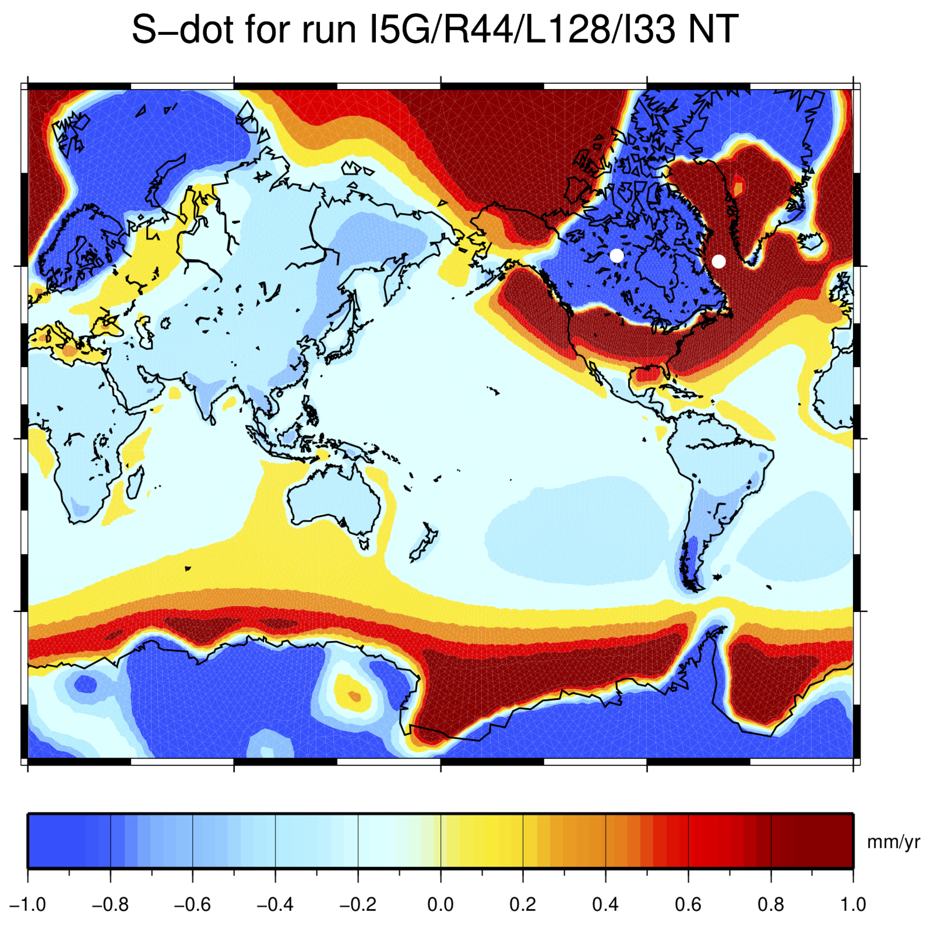
Figure 3 shows the GIA fingerprint , i.e., the rate of present-day relative sea-level change. Assuming that GIA from the melting of past ice sheets is the unique cause of contemporary sea-level change, the rates shown in Figure 3 would be directly observable as constant secular trends at tide gauges (see e.g., [31]). The fingerprint shows the major features and patterns of regional variability already described by Mitrovica and Milne [12], i.e., the strong relative sea-level fall associated with post glacial rebound across the polar regions that where once covered by thick ice sheets and corresponding to RSL zone I of Clark et al. [2], the sea-level rise across the ring-shaped collapsing lateral fore-bulges (zone ), and the region of broad sea-level fall associated with equatorial ocean syphoning (zone V). The offshore sea-level rise clearly evident in the equatorial regions in the GIA maps of Mitrovica and Milne [12] and Melini and Spada [32], and linked to continental levering (zone ), does not stand out clearly in Figure 3, except perhaps along the coasts of central Africa and Australia. In part, this could be due to the different deglaciation chronology and rheology adopted in [12,32], corresponding to model ICE-3G (VM1) of Tushingham and Peltier [54]. However, by a further SELEN run, in which we have still adopted model ICE-5G (VM2) but we have ignored rotational effects as done in [12,32], we have ascertained that the localised offshore sea-level rise is clearly detectable. Thus, we conclude that in Figure 3 this feature is blurred by the long-wavelength effects of Earth rotation. The rotational feedback on sea level is responsible for the southern hemisphere swaths of sea-level rise and fall around Oceania and South America, respectively. In the northern hemisphere, these effects are less evident, due to the dominating contribution of glacial unloading and of the peripheral subsidence.
A crude but useful way to simplify the evident geometrical complexity of GIA fingerprint in Figure 3 is to evaluate its spatial average (all spatial averages of the GIA fingerprints discussed in the following are collected in Table 3). For the ocean-average of , given by , the SLE theory provides an explicit formula, which stems from the constraint of mass conservation. It can be obtained by computing the time-derivative of Equation (22), also taking (23) and (24) into consideration. However, a numerical evaluation on the grid is more convenient, which according to our computations gives the small value
where conventionally we shall use the term small to indicate all GIA rates in modulus. A two-fold larger but coherent value, with =, was computed by Spada [31], who adopted the traditional rotation theory and a coarse three-layer rheological profile for VM2. By inspection of Equations (23) and (24), the small value of may reflect minor variations of the OF associated to changes in the area of the ocean basins, tiny values of the rate of change of the grounded ice mass , or both. Since in model ICE-5G (VM2) the mass distribution over Greenland has seen small but significant variations during the last ≈6000 years that continue to present [55], the average effectively reflects both contributions. However, if we had employed a GIA model that assumes no ice sheets fluctuations during the last few kyrs, like ICE-3G (VM1) [54,56] or ICE-6G (VM5a) [57], also imposing fixed shorelines as in FC76, we would have obtained exactly
as a direct consequence of mass conservation. In fact, this result would be achieved regardless the rheological profile chosen. We note that the SLE theory tells nothing about the whole-Earth-surface average , which however according to our computations in Table 3 is not small.
4.2. Vertical Displacement
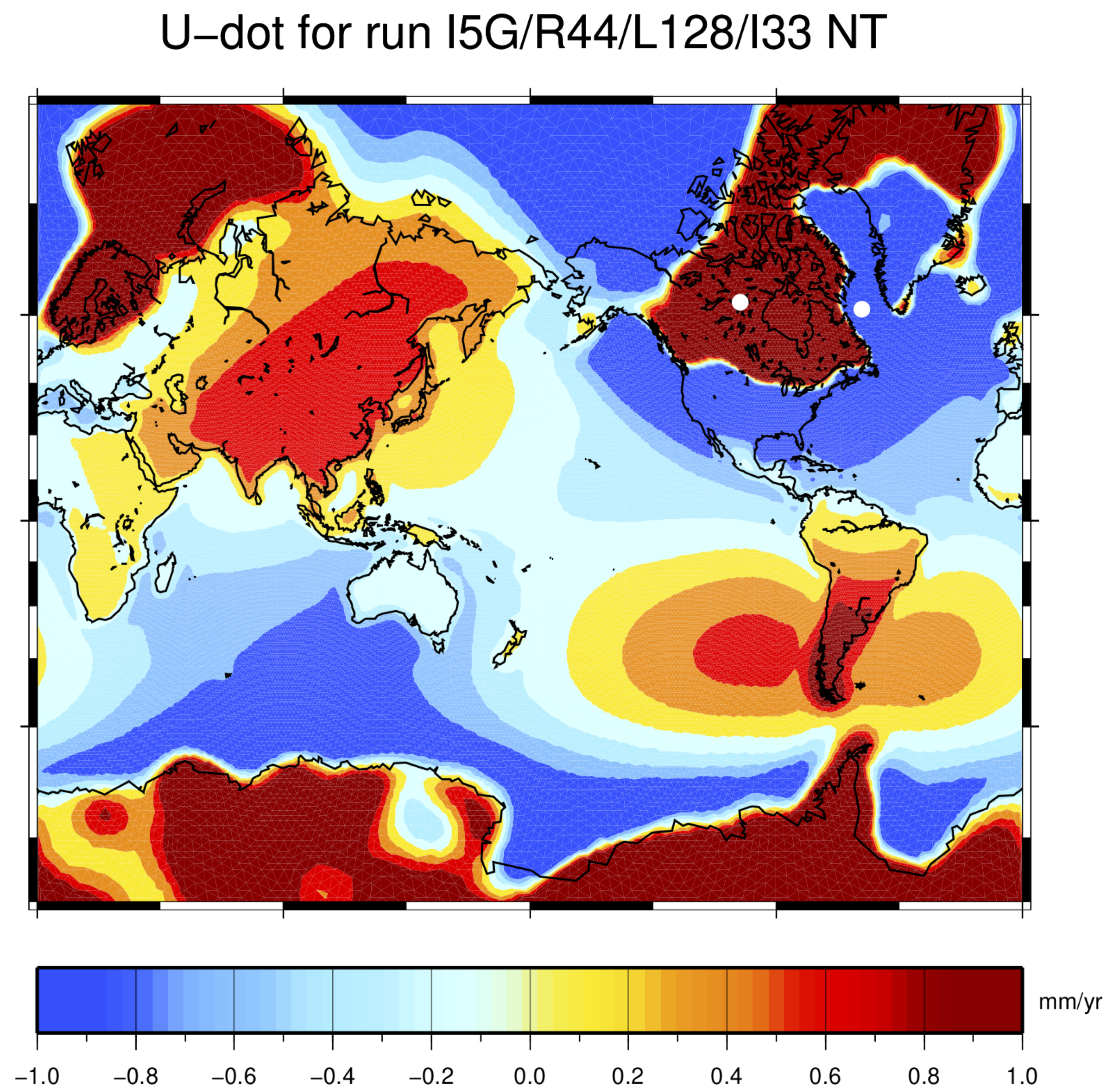
In Figure 4 we show the GIA fingerprint , which represents the present-day rate of change of the vertical displacement that would be observed, at a given location, by an earthbound GPS receiver [58,59,60,61]. By a visual inspection, it is apparent that most of the features of this map are anti-correlated with those shown by fingerprint in Figure 3. In particular, this occurs in previously glaciated areas and in their surroundings, where a relative sea-level rise is accompanied by subsidence, and viceversa. However, we note that apparently paradoxical conditions as having a relative sea-level rise in uplifting regions, or a relative sea-level fall in subsiding regions, are not forbidden a priori by the SLE (see Equation (5)). These conditions may well occur where the rate of absolute change , considered below, attains positive and negative values, respectively.
The anti-correlation between and is not so evident across the equatorial basins, where the fingerprint shows a clear sectorial symmetry of harmonic degree and order , which manifests the long-wavelength effects of Earth rotation. By a comparison with Figure 3, it turns out that such symmetry is definitively more compelling for than for . In the northern hemisphere, the rotation-induced subsidence across North America counteracts the uplift associated with the melting of Laurentide ice sheet, but it intensifies the subsidence across the peripheral fore-bulges. Conversely, in Asia the effects associated to Earth rotation are clearly enhancing the vigor of the uplift induced by continental levering [12]. Interestingly, Figure 4 reveals that a number of GIA-associated processes coherently concur to the uplift in Patagonia, which is caused by local effects due to un-loading of the former Patagonian ice sheet included in model ICE-5G (VM2), by the contribution of continental levering and by the effect from Earth rotation. The unloading associated with the melting of contemporary glaciers and ice caps [62,63], which however is not taken into account in our modeling, would act is the same direction.
As we have done for above, it is useful now to consider spatial averages of the fingerprint in Figure 4. To a very high precision (see Table 3), the whole-Earth average of is numerically found to be
a property of the fingerprint that, once again, is explained in terms of the principle of mass conservation. Since we have assumed a plausible surface load, mass conservation is ensured by Equation (20). From Equation (17), this implies a vanishing at harmonic degree and order , from which the fundamental property (29) of the fingerprint follows immediately. We note that this characteristic is totally unaffected by the choice of the GIA model and, in particular, from the Earth rheological profile assumed. It also holds true when, in GIA modeling, one neglects rotational effects and the horizontal migration of the shorelines, as done for example in the FC76 formulation (this is confirmed by the results in Table 3). Furthermore, as long as the mass conservation constraint is not violated, it is also valid for the fingerprint associated to the present melting of continental ice sheets, for which viscous rheological effects can be neglected [31,34].
We finally note that the SLE theory tells nothing about the GIA-induced average rate of subsidence of the ocean floors , which however according to our computations reported in Table 3, is found not to be small. This would support the idea of a significant influence of climate variations on the isostatic equilibrium of the sea floor topography [64,65]. The negative value of is easily justified by the dominance, in Figure 4, of blue swaths across the oceans caused by the effect of water loading. Conversely, by the argument of mass conservation, we expect a not small and positive value , where superscript c denotes the average over the continents. We shall return on this issue in Section 5 below.
4.3. Geoid Height and Absolute Sea-Level Change
In Figure 5 we show the map of the GIA fingerprint for . According to Equation (9), this quantity represents the present-day rate of change of the geoid height. It appears that is characterized by a well developed lobed symmetry with and, with respect to and , by an overall smoother resemblance. The cause is to be found in the different spectral content of the and loading Love numbers that contribute to and , respectively; see SM19 for details. The pattern associated to Earth rotation is so strong that the regional effects from glacial unloading are only just visible in the polar regions of both hemispheres. To suitably interpret the symmetry, it is worth to note that according to our computations, the GIA-induced polar motion presently occurs at a rate of ∼1.4 deg/Myr (roughly corresponding to 15 cm/year on the Earth’s surface) along the meridian ∼80 W (roughly, towards the Hudson Bay). Such rate and direction of polar drift match well the astronomical observations in the course of last century (see e.g., Lambeck [4]) and with recent analyses about the causes of secular polar motion [66]. Performing a further run of SELEN in which we have adopted the traditional rotation theory (see e.g., Spada et al. [46]), we have verified that the pattern of would be indeed much stronger, with a more than two-fold rate of polar drift of ∼3.5 deg/Myr in the same direction. The enhanced rate of polar motion implied by the traditional rotation theory compared to the new theory is in full agreement with the analysis of Mitrovica et al. [51] and Mitrovica and Wahr [52].
Based upon the same argument we have used for above (i.e., mass conservation ensured by plausible surface loads), the fundamental property of the fingerprint can be similarly expressed by
which we have verified numerically to be valid to a very high precision (see Table 3). In consequence of (30), harmonics with are not contributing to . We further note that condition , suggested by the results in column (a) of Table 3, is due to chance and it is not reflecting any particular property of the GIA fingerprints. Indeed, when the traditional rotation theory is adopted or rotation is neglected, as done in columns (b) and (c), respectively, or alternative GIA models such as ICE-6G (VM5a) are employed as in SM19, this condition is not met.
As shown by e.g., Melini and Spada [32], the individual harmonic components of , i.e., , are proportional to the rates of change of the GIA-induced variations of the Stokes coefficients of the Earth’s gravity field, detectable by the Gravity Recovery and Climate Experiment (GRACE); see Wahr et al. [67] for a discussion. In particular,
where and are the GIA-induced variations of the fully normalised cosine and sine Stokes coefficients, is the imaginary unit, a is the reference Earth’s radius, is the Kronecker delta, and the asterisk denotes complex conjugation. We also note that since we are solving the SLE in a geocentric reference frame with origin in the whole-Earth center of mass, a further property of the field is that of not including contributions from the harmonics of degree and order and [68]. Hence, in Equation (31), only terms with harmonic degree appear.
The GIA fingerprint for , shown in Figure 6, represents the present-day rate of change of the sea surface height (or absolute sea level) that would be observed across the oceans by satellite altimetry [22,31], assuming that only GIA is contributing to contemporary sea-level change. It is worth to recall that, regardless the rotation theory adopted in GIA modeling, the fingerprint is not independent upon and , since from the basic form of the SLE (see Equation (5)), we have . Actually, in view of the relatively small range of values spanned by , which never exceeds the value of mm year in modulus, the approximation of the SLE is inviting, but it would be an oversimplification. We further note that only in the idealized case of an un-deformable Earth, with , absolute and relative sea-level variations would coincide, with .
By the FC76 formula, it turns out that (see Equation (6) and Figure 1) is strongly associated to the rate of geoid change, since it simply differs from by the spatially invariant quantity , where c is the FC76 constant. In consequence of the FC76 formula, the whole-Earth surface average of is
which turns out to be an appealingly simple definition of . Using the gridded data shown in Figure 6, we numerically obtain a not small ocean average
a (GIA model dependent) value closely matching the value of , often adopted as a rule of thumb to correct the altimetric absolute sea-level trend for the effects of past GIA (see [31,34] and references therein). Since during the altimetry era (1992-today) the rate of global mean sea-level rise has well exceeded ∼3 mm year [69,70], using the average (33) to perform the GIA correction is certainly justified. However, spatial trends of at a regional scale may become important when one considers the effects of present land ice on absolute sea level change, as done by Ponte et al. [71].
4.4. Surface Load
We conclude our overview with a few remarks about the GIA fingerprint for , the present-day rate of change of the surface load. This quantity, which is shown in Figure 7 in units of of water equivalent, describes the local variations in the distribution of the ice and water. We recall that the load variation is defined as , where is given by Equation (21) and is the value of L in the reference state (see Figure 1). To interpret the gross features of the map shown in Figure 7, for one moment it is convenient to assume that the continent function C and the ocean function O are constant to the present day values, as it would be implicit in the FC76 formulation of GIA. If this holds true, by evaluating the time-derivative of Equation (21) at present time we obtain
where is the ice thickness variation and we have also used the definition of sea-level change given by Equation (4). Across the oceans, the existence of the positive correlation between and predicted by Equation (34) is easily recognized comparing the fingerprints in Figure 3 and Figure 7. The strong contribution to across Greenland is associated with the current ice variation that ICE-5G (VM2) embodies in this region [44,55]; in all other continental areas the load variation vanishes, in agreement to Equation (34). A notable exception is West Antarctica, where the negative trend of the load is associated with the significant variations of the ocean function in this region, associated with the still continuing transition between grounded and floating ice. However, this is not accounted for in the FC76 approximation (34), which assumes a constant OF. Lastly, we observe that once integrated over the whole Earth’s surface, gives the global mass change of the system with respect to the reference state. However, since mass is conserved, consistently with Equation (19), we have
which according to Table 3 is numerically verified to a very high precision.
5. Observing the Global GIA Fingerprint by Vertical GPS Rates
As an example of application of the fingerprints properties illustrated above, we mention the problem of directly using geodetic observations to quantify the present global pattern of GIA. Recently, using a large global compilation of geodetic GPS rates in conjunction with a Bayesian inference method, Husson et al. [72] have reconstructed and visualized the long-wavelength signature of GIA on the rate of present day vertical crustal uplift. In principle, once the contributions from short-wavelength tectonic phenomena have been filtered out, the geodetically observed rates across the continents should match those predicted by current GIA models, at least in their global traits and in their spatial averages. One possible way to verify this consistency is to consider the average over the continents of the geodetically determined rate of vertical uplift , where , being the area of the continents. In Husson et al. [72], the scalar field has been estimated from GPS vertical rates by a self-adaptive trans-dimensional regression that exploits the properties of the Voronoi tesselation. The pattern of GIA inferred by regression has been found to broadly resemble the one that we would expect by a model like ICE-5G (VM2), provided that components with wavelengths <2500 km are removed.
Of course, the average could be evaluated numerically using the results of Figure 4 and compared to the value obtained from the pattern of the GPS rates. However, through the SLE, it is straightforward and possibly more meaningful to express in terms of the ocean-averaged fingerprints and that we have already discussed above in view of their particular significance. Here we largely follow Husson et al. [72] and, since we simply aim at illustrating the method, we do not consider the modeling uncertainties on the GIA fingerprints. On one hand, taking advantage of Equation (29), we have
which by the additivity of the surface average gives
or, equivalently,
where we have used the definitions of continent and ocean average; hence
On the other hand, ocean-averaging both sides of the SLE in the form (5) gives
which used into (39) yields the average of across the continents
which is only expressed in terms of ocean-averaged fingerprints.
The exercise above shows that the average vertical uplift across the continents determined by GPS could be estimated, in principle, by ocean-averaging the tide gauge trends and subtracting the ocean averaged altimetry-derived rate of absolute sea-level change. This would hold true regardless the GIA model employed. By approximating and , so that , and using the ocean averages for ICE-5G (VM2) given by Equations (27) and (33), we obtain the not small value
where we note that since in Equation (41) Husson et al. [72] have used the crude fixed-shorelines approximation that implies they have obtained slightly different values for . Nevertheless, the value of matches very well the rate effectively reconstructed by Husson et al. [72] . This suggests that the trans-dimensional regression method has been effective in isolating the fingerprint of GIA. As pointed by Husson et al. [72], the effects of current melting of glaciers and ice caps in response to global warming would not alter substantially our estimate in (42).
6. Conclusions
In this work we have reviewed some aspects of GIA, i.e., the response of the Earth to the disequilibrium caused by the melting of the late-Pleistocene ice sheets. Arguments based upon the physical properties of the SLE have been corroborated by results obtained from up-to-date numerical tools in GIA modeling. Among the processes that concur to present sea-level rise, the special role of GIA has been recognized long ago; in fact, only GIA is affected by the rheology of the Earth and, at the same time, it affects significantly the gravity field and the rotational state of the planet. Although, according to GIA models, the deglaciation of the late-Pleistocene ice sheets came to an end thousands of years ago, at present the effects of GIA are still significant and they influence a number of directly observable geophysical and geodetic quantities. Since GIA evolves slowly, its contribution to the instrumental observations will persist also during next centuries although it shall gradually fade away. Model predictions show that the computed patterns or fingerprints of GIA are characterized by an outstanding complexity. In our roundup of the general properties of the GIA fingerprints, we have considered both the geometrical and the physical aspects of such complexity, emphasizing their spatial symmetries and regional character, which we have interpreted qualitatively and quantitatively with the aid of the SLE.
The study of the relative sea level fingerprint has revealed that at present the role of GIA is not that of causing an effective, mean global change. Rather, it causes essentially local regional effects which strongly contaminate the tide gauges records but that almost wash out when averaged over the present-day oceans, leaving a small contribution reflecting minor variations in the area of the sea floor and possibly current variations of ice thickness, when these are accounted for by the GIA model. The coastal regions are certainly those being most affected by the regional variability of GIA. The pattern of the GIA-induced vertical uplift is extremely variegated but it globally averages out to zero as an effect of mass conservation. Although it is largely anti-correlated to that of relative sea level, it shows more clearly the mark of the rotational effects of GIA, with a symmetry dominated by a very long-wavelength harmonic pattern. By a specific example from the recent literature, we have shown that the basic traits of the GIA fingerprint of vertical displacement can be visualized using data from a large global compilation of geodetic GPS rates. The symmetry imposed by the polar drift of the rotation axis is even more enhanced when one considers the fingerprints of the geoid height variation and of the absolute sea-level change, which only differ by a spatially invariant term. These two last signatures of GIA have presently a particular role in physical geodesy, since they are commonly employed to purge the trends of the Stokes coefficients of the gravity field and the sea-level altimetric records from the GIA effects.
In this study, we have employed only one of the ICE-X models of WR Peltier and collaborators [44], leaving a systematic exploration to a further study. Unquestionably, the shapes of the GIA fingerprints are significantly affected by the choice of the deglaciation chronology and of the rheological profile. An idea of this sensitivity can be obtained comparing directly the results obtained here and based on ICE-5G (VM2) with those of SM19, who have adopted a realization of ICE-6G (VM5a) [57]. In [32], it is possible to visualize the GIA fingerprints for old model ICE-3G (VM1) of Tushingham and Peltier [54], which differs from the most recent ICE-X models for a significantly larger meltwater release from Antarctica. For a discussion about the relationship between the fingerprints shapes and the GIA models employed, see in particular Spada and Galassi [73], who have emphasized how the choice of the model affects the GIA corrections at tide gauges and, consequently, the estimate of secular sea-level rise. Of course, GIA models that are independent from the ICE-X models exist and have a central role in the literature, like those progressively developed at the National Australian University by Kurt Lambeck and colleagues (see Nakada and Lambeck [74], Lambeck et al. [75] and subsequent contributions). Some GIA fingerprints for one of these models are shown in [32].
Recent reviews [31,76] have indicated that the evolution of the GIA models has been considerable during last decades, because of the increased availability of proxy data constraining the history of sea level in the last thousand years [31,34]. Such evolution has also motivated efforts aimed at extracting geophysical information from ensembles (or more often mini-ensembles) of GIA models, as done by e.g., [32,77,78,79,80,81,82]. The evolution of GIA models shall certainly continue in the future, in order to account for more realistic (possibly three-dimensional) descriptions of the Earth’s rheology, to include new details of the history of the ice sheets and their distribution, to relax some simplifying assumptions in the theory behind the SLE, to further fine-tune the rotation theory, and to add new elements or new branches to the interactions diagram of Figure 1. Thus, although their general properties associated to the principle of mass conservation shall not change, the shape of the GIA fingerprints is certainly not given once and for all.
Author Contributions
G.S. and D.M. have equally contributed to the development of the theory, to the numerical experiments, and to the writing of the manuscript.
Funding
G.S. is funded by a FFABR (Finanziamento delle Attività Base di Ricerca) grant of MIUR (Ministero dell’Istruzione, dell’Università e della Ricerca) and by a research grant of Dipartimento di Scienze Pure e Applicate (DiSPeA) of the University of Urbino “Carlo Bo”.
Acknowledgments
Program SELEN (SELEN version 4.0) is available from Zenodo at the link https:// zenodo.org/ record/3377404 (doi:10.5281/ zenodo.3339209) and from the Computational Infrastructure for Geodynamics (CIG) at github.com/ geodynamics/selen. The open source Love numbers calculator and Post Glacial Rebound Solver TABOO can be downloaded from https://github.com/danielemelini/TABOO. Some of the figures have been drawn using the Generic Mapping Tools (GMT) of Wessel and Smith [83]. We thank Gaia Galassi and Marco Olivieri for their advice and encouragement. We thank Francesco Mainardi for insightful discussion about the rheological aspects of GIA and for warm hospitality. G.S. has benefited from the serene atmosphere of the Naturalistic Annex of the Museum of Bagnacavallo (RA), Italy, where this paper has been conceived. Raffaello Mascetti has patiently revised the manuscript during various stages of its development, providing constructive comments and invaluable inspiration.
Conflicts of Interest
The authors declare no conflict of interest.
References
- Farrell, W.; Clark, J. On postglacial sea-level. Geophys. J. R. Astr. Soc. 1976, 46, 647–667. [Google Scholar] [CrossRef]
- Clark, J.A.; Farrell, W.E.; Peltier, W.R. Global changes in postglacial sea level: A numerical calculation. Quat. Res. 1978, 9, 265–287. [Google Scholar] [CrossRef]
- Conrad, C. The solid earth’s influence on sea level. Bull. Geol. Soc. Am. 2013, 125, 1027–1052. [Google Scholar] [CrossRef]
- Lambeck, K. The Earth’s Variable Rotation: Geophysical Causes And Consequences; Cambridge University Press: Cambridge, UK, 1980. [Google Scholar]
- Peltier, W. Global sea level rise and glacial isostatic adjustment. Glob. Planet. Chang. 1999, 20, 93–123. [Google Scholar] [CrossRef]
- Woodward, R. On the form and position of mean sea level. USGS Bull. 1888, 48, 87–170. [Google Scholar]
- Daly, R.A. Pleistocene changes of level. Am. J. Sci. 1925, 10, 281–313. [Google Scholar] [CrossRef]
- Walcott, R. Past sea levels, eustasy and deformation of the earth. Quat. Res. 1972, 2, 1–14. [Google Scholar] [CrossRef]
- Suess, E. Face of the Earth; Clarendon Press: Oxford, UK, 1906. [Google Scholar]
- Milne, G.A.; Mitrovica, J.X. Searching for eustasy in deglacial sea-level histories. Quat. Sci. Rev. 2008, 27, 2292–2302. [Google Scholar] [CrossRef]
- Gregory, J.M.; Griffies, S.M.; Hughes, C.W.; Lowe, J.A.; Church, J.A.; Fukimori, I.; Gomez, N.; Kopp, R.E.; Landerer, F.; Le Cozannet, G.; et al. Concepts and terminology for sea level: Mean, variability and change, both local and global. Surv. Geophys. 2019, 1–39. [Google Scholar] [CrossRef]
- Mitrovica, J.; Milne, G. On the origin of late Holocene sea-level highstands within equatorial ocean basins. Quat. Sci. Rev. 2002, 21, 2179–2190. [Google Scholar] [CrossRef]
- Clark, P.U.; Mitrovica, J.; Milne, G.; Tamisiea, M. Sea-level fingerprinting as a direct test for the source of global meltwater pulse IA. Science 2002, 295, 2438–2441. [Google Scholar]
- Kendall, R.A.; Mitrovica, J.X.; Milne, G.A.; Törnqvist, T.E.; Li, Y. The sea-level fingerprint of the 8.2 ka climate event. Geology 2008, 36, 423–426. [Google Scholar] [CrossRef]
- Mitrovica, J.; Gomez, N.; Morrow, E.; Hay, C.; Latychev, K.; Tamisiea, M. On the robustness of predictions of sea level fingerprints. Geophys. J. Int. 2011, 187, 729–742. [Google Scholar] [CrossRef] [Green Version]
- Stocchi, P.; Spada, G. Glacio and hydro-isostasy in the Mediterranean Sea: Clark zones and role of remote ice sheets. Ann. Geophys. 2007, 50. [Google Scholar] [CrossRef]
- Mauz, B.; Ruggieri, G.; Spada, G. Terminal Antarctic melting inferred from a far-field coastal site. Quat. Sci. Rev. 2015, 116, 122–132. [Google Scholar] [CrossRef]
- Lambeck, K.; Chappell, J. Sea level change through the last glacial cycle. Science 2001, 292, 679–686. [Google Scholar] [CrossRef]
- Plag, H.P.; Jüettner, H.U. Inversion of global tide gauge data for present-day ice load changes (scientific paper). Mem. Natl. Inst. Polar Res. Spec. Issue 2001, 54, 301–317. [Google Scholar]
- Douglas, B. Concerning evidence for fingerprints of glacial melting. J. Coast. Res. 2008, 24, 218–227. [Google Scholar] [CrossRef]
- Spada, G.; Galassi, G. Spectral analysis of sea-level during the altimetry era, and evidence for GIA and glacial melting fingerprints. Glob. Planet. Chang. 2015, 143, 34–49. [Google Scholar] [CrossRef]
- Cazenave, A.; Llovel, W. Contemporary sea level rise. Annu. Rev. Mar. Sci. 2010, 2, 145–173. [Google Scholar] [CrossRef]
- Bamber, J.; Riva, R. The sea level fingerprint of recent ice mass fluxes. Cryosphere 2010, 4, 621–627. [Google Scholar] [CrossRef] [Green Version]
- Kopp, R.; Mitrovica, J.; Griffies, S.; Yin, J.; Hay, C.; Stouffer, R. The impact of Greenland melt on local sea levels: A partially coupled analysis of dynamic and static equilibrium effects in idealized water-hosing experiments. Clim. Chang. 2010, 103, 619–625. [Google Scholar] [CrossRef]
- Riva, R.E.; Bamber, J.L.; Lavallée, D.A.; Wouters, B. Sea-level fingerprint of continental water and ice mass change from GRACE. Geophys. Res. Lett. 2010, 37. [Google Scholar] [CrossRef] [Green Version]
- Hay, C.C.; Morrow, E.; Kopp, R.E.; Mitrovica, J.X. Probabilistic reanalysis of twentieth-century sea-level rise. Nature 2015, 517, 481. [Google Scholar] [CrossRef] [PubMed]
- Adhikari, S.; Ivins, E.R.; Frederikse, T.; Landerer, F.W.; Caron, L. Sea-level fingerprints emergent from GRACE mission data. Earth Syst. Sci. Data 2019, 11, 629–646. [Google Scholar] [CrossRef] [Green Version]
- Mitrovica, J.X.; Gomez, N.; Clark, P.U. The sea-level fingerprint of West Antarctic collapse. Science 2009, 323, 753. [Google Scholar] [CrossRef]
- Spada, G.; Bamber, J.; Hurkmans, R. The gravitationally consistent sea-level fingerprint of future terrestrial ice loss. Geophys. Res. Lett. 2013, 40, 482–486. [Google Scholar] [CrossRef] [Green Version]
- Galassi, G.; Spada, G. Sea-level rise in the Mediterranean Sea by 2050: Roles of terrestrial ice melt, steric effects and glacial isostatic adjustment. Glob. Planet. Chang. 2014, 123, 55–66. [Google Scholar] [CrossRef]
- Spada, G. Glacial Isostatic Adjustment and Contemporary Sea Level Rise: An Overview. Surv. Geophys. 2017, 38, 1–33. [Google Scholar] [CrossRef]
- Melini, D.; Spada, G. Some remarks on Glacial Isostatic Adjustment modelling uncertainties. Geophys. J. Int. 2019, 218, 401–413. [Google Scholar] [CrossRef]
- Spada, G.; Melini, D. SELEN4 (SELEN version 4.0): A Fortran program for solving the Gravitationally topographically Self-Consistent Sea Level Equ. Glacial Isostatic Adjust. Model. Geosci. Model Dev. 2019. [Google Scholar] [CrossRef]
- Tamisiea, M.E. Ongoing glacial isostatic contributions to observations of sea level change. Geophys. J. Int. 2011, 186, 1036–1044. [Google Scholar] [CrossRef]
- Farrell, W. Deformation of the Earth by surface loads. Rev. Geophys. 1972, 10, 761–797. [Google Scholar] [CrossRef]
- Milne, G.A.; Mitrovica, J.X. Postglacial sea-level change on a rotating Earth. Geophys. J. Int. 1998, 133, 1–19. [Google Scholar] [CrossRef] [Green Version]
- Han, D.; Wahr, J. Post-glacial rebound analysis for a rotating Earth. In Slow Deformations and Transmission of Stress in the Earth; Cohen, S., Vanicek, P., Eds.; AGU Mono. Series 49; American Geophysical Union: Washington, DC, USA, 1989; pp. 1–6. [Google Scholar]
- Jerri, A. Introduction to Integral Equations with Applications; John Wiley & Sons: Hoboken, NJ, USA, 1999. [Google Scholar]
- Mitrovica, J.X.; Peltier, W. On postglacial geoid subsidence over the equatorial oceans. J. Geophys. Res. Solid Earth 1991, 96, 20053–20071. [Google Scholar] [CrossRef]
- Mitrovica, J.X.; Milne, G.A. On post-glacial sea level: I. General theory. Geophys. J. Int. 2003, 154, 253–267. [Google Scholar] [CrossRef] [Green Version]
- Spada, G.; Stocchi, P. SELEN: A Fortran 90 program for solving the “Sea Level Equation”. Comput. Geosci. 2007, 33, 538–562. [Google Scholar] [CrossRef]
- Spada, G.; Stocchi, P. The Sea Level Equation, Theory and Numerical Examples; Aracne: Roma, Italy, 2006. [Google Scholar]
- Tegmark, M. An icosahedron-based method for pixelizing the celestial sphere. Astrophys. J. 1996, 470, L81. [Google Scholar] [CrossRef]
- Peltier, W. Global glacial isostasy and the surface of the ice-age Earth: The ICE-5G (VM2) model and GRACE. Annu. Rev. Earth Planet. Sci. 2004, 32, 111–149. [Google Scholar] [CrossRef]
- Dziewonski, A.M.; Anderson, D.L. Preliminary reference Earth model. Phys. Earth Planet. Inter. 1981, 25, 297–356. [Google Scholar] [CrossRef]
- Spada, G.; Barletta, V.R.; Klemann, V.; Riva, R.; Martinec, Z.; Gasperini, P.; Lund, B.; Wolf, D.; Vermeersen, L.; King, M. A benchmark study for glacial isostatic adjustment codes. Geophys. J. Int. 2011, 185, 106–132. [Google Scholar] [CrossRef] [Green Version]
- Spada, G. ALMA, a Fortran program for computing the viscoelastic Love numbers of a spherically symmetric planet. Comput. Geosci. 2008, 34, 667–687. [Google Scholar] [CrossRef]
- Peltier, W.R. Ice age paleotopography. Science 1994, 265, 195–201. [Google Scholar] [CrossRef] [PubMed]
- Amante, C.; Eakins, B.W. ETOPO1 Arc-Minute Global Relief Model: Procedures, Data Source and Analysis; Technical Report; NOAA: Washington, DC, USA, 2009. [CrossRef]
- Eakins, B.; Sharman, G. Hypsographic curve of Earth’s surface from ETOPO1; NOAA National Geophysical Data Center: Boulder, CO, USA, 2012. [Google Scholar]
- Mitrovica, J.X.; Wahr, J.; Matsuyama, I.; Paulson, A. The rotational stability of an ice-age earth. Geophys. J. Int. 2005, 161, 491–506. [Google Scholar] [CrossRef] [Green Version]
- Mitrovica, J.X.; Wahr, J. Ice Age Earth Rotation. Annu. Rev. Earth Planet. Sci. 2011, 39, 577–616. [Google Scholar] [CrossRef]
- Spada, G.; Olivieri, M.; Galassi, G. Anomalous secular sea-level acceleration in the Baltic Sea caused by isostatic adjustment. Ann. Geophys. 2014, 57, S0432. [Google Scholar]
- Tushingham, A.; Peltier, W. ICE-3G—A new global model of late Pleistocene deglaciation based upon geophysical predictions of post-glacial relative sea level change. J. Geophys. Res. 1991, 96, 4497–4523. [Google Scholar] [CrossRef]
- Tarasov, L.; Richard Peltier, W. Greenland glacial history and local geodynamic consequences. Geophys. J. Int. 2002, 150, 198–229. [Google Scholar] [CrossRef] [Green Version]
- Tushingham, A.; Peltier, W. Validation of the ICE-3G model of Würm-Wisconsin deglaciation using a global data base of relative sea level histories. J. Geophys. Res. 1992, 97, 3285–3304. [Google Scholar] [CrossRef]
- Peltier, W.; Argus, D.; Drummond, R.; Moore, A. Postglacial rebound and current ice loss estimates from space geodesy: The new ICE-6G (VM5a) global model. In Proceedings of the AGU Fall Meeting Abstracts, San Francisco, CA, USA, 3–7 December 2012; Volume 1, p. 2. [Google Scholar]
- Wöppelmann, G.; Miguez, B.M.; Bouin, M.N.; Altamimi, Z. Geocentric sea-level trend estimates from GPS analyses at relevant tide gauges world-wide. Glob. Planet. Chang. 2007, 57, 396–406. [Google Scholar] [CrossRef] [Green Version]
- Wöppelmann, G.; Marcos, M. Vertical land motion as a key to understanding sea level change and variability. Rev. Geophys. 2016, 54, 64–92. [Google Scholar] [CrossRef]
- Pfeffer, J.; Allemand, P. The key role of vertical land motions in coastal sea level variations: A global synthesis of multisatellite altimetry, tide gauge data and GPS measurements. Earth Planet. Sci. Lett. 2016, 439, 39–47. [Google Scholar] [CrossRef]
- Pfeffer, J.; Spada, G.; Mémin, A.; Boy, J.P.; Allemand, P. Decoding the origins of vertical land motions observed today at coasts. Geophys. J. Int. 2017, 210, 148–165. [Google Scholar] [CrossRef]
- Ivins, E.R.; James, T.S. Simple models for late Holocene and present-day Patagonian glacier fluctuations and predictions of a geodetically detectable isostatic response. Geophys. J. Int. 1999, 138, 601–624. [Google Scholar] [CrossRef] [Green Version]
- Rostami, K.; Peltier, W.; Mangini, A. Quaternary marine terraces, sea-level changes and uplift history of Patagonia, Argentina: Comparisons with predictions of the ICE-4G (VM2) model of the global process of glacial isostatic adjustment. Quat. Sci. Rev. 2000, 19, 1495–1525. [Google Scholar] [CrossRef]
- Crowley, J.W.; Katz, R.F.; Huybers, P.; Langmuir, C.H.; Park, S.H. Glacial cycles drive variations in the production of oceanic crust. Science 2015, 347, 1237–1240. [Google Scholar] [CrossRef] [Green Version]
- Conrad, C.P. How climate influences sea-floor topography. Science 2015, 347, 1204–1205. [Google Scholar] [CrossRef] [Green Version]
- Adhikari, S.; Caron, L.; Steinberger, B.; Reager, J.T.; Kjeldsen, K.K.; Marzeion, B.; Larour, E.; Ivins, E.R. What drives 20th century polar motion? Earth Planet. Sci. Lett. 2018, 502, 126–132. [Google Scholar] [CrossRef] [Green Version]
- Wahr, J.; Molenaar, M.; Bryan, F. Time variability of the Earth’s gravity field: Hydrological and oceanic effects and their possible detection using GRACE. J. Geophys. Res. Solid Earth 1998, 103, 30205–30229. [Google Scholar] [CrossRef]
- Hofmann-Wellenhof, B.; Moritz, H. Physical Geodesy; Springer Science & Business Media: Berlin, Germany, 2006. [Google Scholar]
- Church, J.; Clark, P.; Cazenave, A.; Gregory, J.; Jevrejeva, S.; Levermann, A.; Merrifield, M.; Milne, G.; Nerem, R.; Nunn, P.; et al. Climate Change 2013: The Physical Science Basis. Contribution of Working Group I to the Fifth Assessment Report of the Intergovernmental Panel on Climate Change. In Sea Level Change; Stocker, T., Qin, D., Plattner, G.K., Tignor, M., Allen, S., Boschung, J., Nauels, A., Xia, Y., Bex, V., Midgley, P., Eds.; Cambridge University Press: Cambridge, UK, 2013; pp. 1138–1191. [Google Scholar]
- Slangen, A.B.; Meyssignac, B.; Agosta, C.; Champollion, N.; Church, J.A.; Fettweis, X.; Ligtenberg, S.R.; Marzeion, B.; Melet, A.; Palmer, M.D.; et al. Evaluating model simulations of twentieth-century sea level rise. Part I: Global mean sea level change. J. Clim. 2017, 30, 8539–8563. [Google Scholar] [CrossRef]
- Ponte, R.M.; Quinn, K.J.; Piecuch, C.G. Accounting for gravitational attraction and loading effects from land ice on absolute sea level. J. Atmos. Ocean. Technol. 2018, 35, 405–410. [Google Scholar] [CrossRef]
- Husson, L.; Bodin, T.; Spada, G.; Choblet, G.; Kreemer, C. Bayesian surface reconstruction of geodetic uplift rates: Mapping the global fingerprint of Glacial Isostatic Adjustment. J. Geodyn. 2018, 122, 25–40. [Google Scholar] [CrossRef]
- Spada, G.; Galassi, G. New estimates of secular sea level rise from tide gauge data and GIA modelling. Geophys. J. Int. 2012, 191, 1067–1094. [Google Scholar] [CrossRef] [Green Version]
- Nakada, M.; Lambeck, K. Glacial rebound and relative sea-level variations: A new appraisal. Geophys. J. Int. 1987, 90, 171–224. [Google Scholar] [CrossRef]
- Lambeck, K.; Purcell, A.; Johnston, P.; Nakada, M.; Yokoyama, Y. Water-load definition in the glacio-hydro-isostatic sea-level equation. Quat. Sci. Rev. 2003, 22, 309–318. [Google Scholar] [CrossRef]
- Whitehouse, P.L. Glacial isostatic adjustment modelling: Historical perspectives, recent advances, and future directions. Earth Surf. Dyn. 2018, 6, 401–429. [Google Scholar] [CrossRef]
- Guo, J.; Huang, Z.; Shum, C.; van der Wal, W. Comparisons among contemporary glacial isostatic adjustment models. J. Geodyn. 2012, 61, 129–137. [Google Scholar] [CrossRef]
- Spada, G.; Ruggieri, G.; Sørensen, L.S.; Nielsen, K.; Melini, D.; Colleoni, F. Greenland uplift and regional sea level changes from ICESat observations and GIA modelling. Geophys. J. Int. 2012, 189, 1457–1474. [Google Scholar] [CrossRef] [Green Version]
- Huang, Z. The Role of Glacial Isostatic Adjustment (GIA) Process On the Determination of Present-Day Sea-Level Rise; The Ohio State University: Columbus, OH, USA, 2013. [Google Scholar]
- Hay, C.C.; Morrow, E.; Kopp, R.E.; Mitrovica, J.X. Estimating the sources of global sea level rise with data assimilation techniques. Proc. Natl. Acad. Sci. USA 2013, 110, 3692–3699. [Google Scholar] [CrossRef]
- Jevrejeva, S.; Moore, J.; Grinsted, A.; Matthews, A.; Spada, G. Trends and acceleration in global and regional sea levels since 1807. Glob. Planet. Chang. 2014, 113, 11–22. [Google Scholar] [CrossRef] [Green Version]
- Caron, L.; Ivins, E.; Larour, E.; Adhikari, S.; Nilsson, J.; Blewitt, G. GIA model statistics for GRACE hydrology, cryosphere, and ocean science. Geophys. Res. Lett. 2018, 45, 2203–2212. [Google Scholar] [CrossRef]
- Wessel, P.; Smith, W.H.F. New, improved version of Generic Mapping Tools released. Eos Trans. Am. Geophys. Union 1998, 79, 579. [Google Scholar] [CrossRef]
Figure 1.
Sketches of the reference state for time (a) and of the general configuration for (b) showing the three Earth’s portions that are interacting in the SLE: the solid Earth, the oceans and the ice sheets. With r we denote the radius of a given point relative to the center of mass of the whole Earth system. Changes in sea level relative to the solid Earth are observed by the red stick meter. The sea surface is equipotential in (a) but also in (b), after that the ice sheets have shrunk and the mass of the oceans has consequently varied to compensate exactly the ice mass loss. The vertical arrows in (b) indicate that the sea surface and the solid Earth have moved relative to the origin of the reference frame. The spring-dashpot system is an exemplification of Earth’s rheology.

Figure 2.
The top part of the triangle shows the elements that are perpetually interacting in the SLE (the solid Earth, the ice sheets and the oceans) through surface loading and mutual gravitational attraction. The bottom part qualitatively shows how Earth rotational effects are coming into play. The figure is inspired to that originally published by Clark et al. [2].

Figure 3.
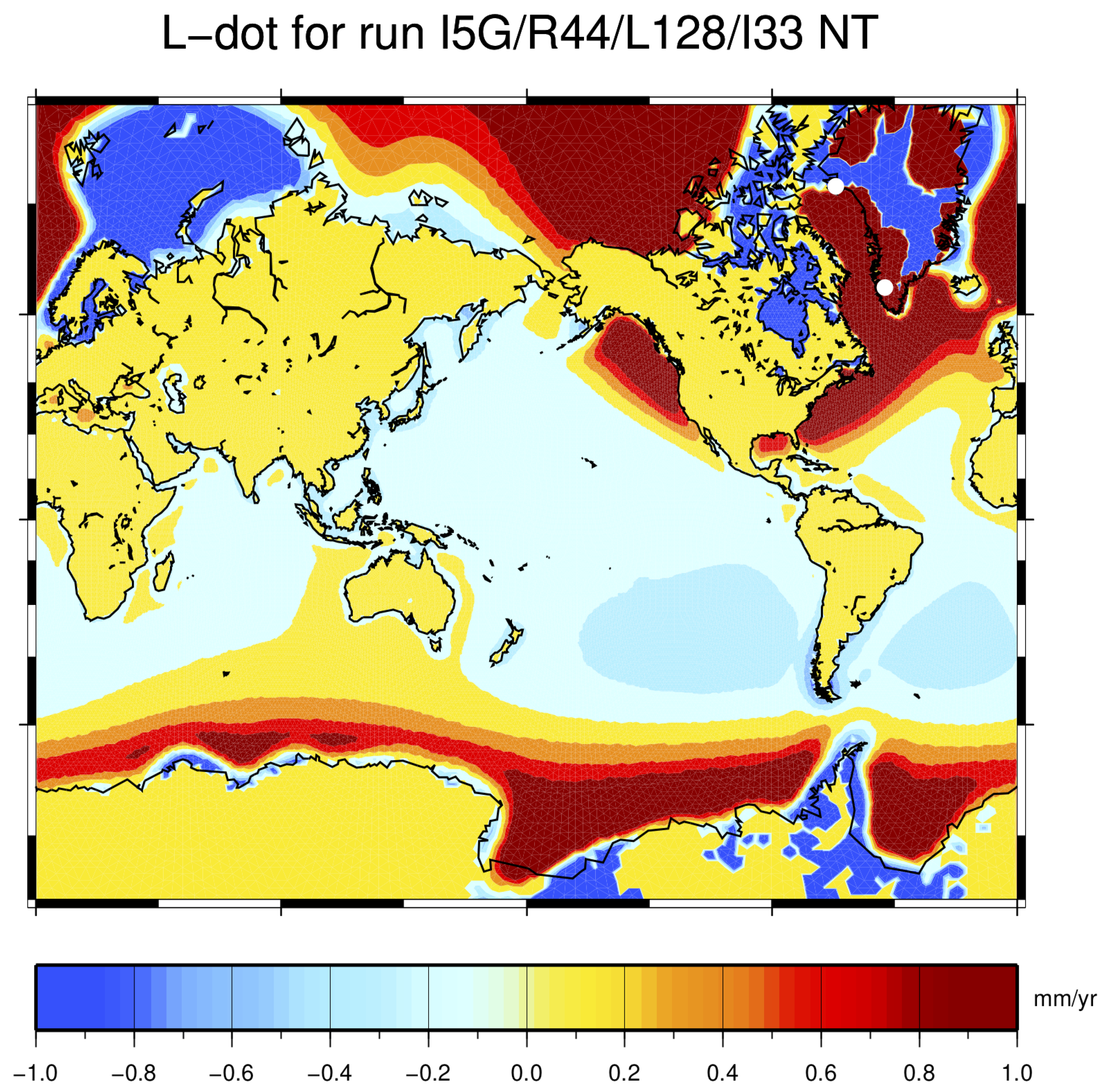
GIA fingerprint for , the present-day rate of relative sea-level change, obtained by implementing model ICE-5G (VM2) in SELEN. To better visualize the regional variations, the palette is limited to the range of mm year. The largest rates, marked by white dots, are associated with the isostatic disequilibrium still caused by the disintegration of the Laurentide ice sheet complex, with and mm year, respectively. The most significant regional variability, measured as the density of local maxima and minima of in this map, is found to within ∼1500 km from the continental margins.
Figure 3.
GIA fingerprint for , the present-day rate of relative sea-level change, obtained by implementing model ICE-5G (VM2) in SELEN. To better visualize the regional variations, the palette is limited to the range of mm year. The largest rates, marked by white dots, are associated with the isostatic disequilibrium still caused by the disintegration of the Laurentide ice sheet complex, with and mm year, respectively. The most significant regional variability, measured as the density of local maxima and minima of in this map, is found to within ∼1500 km from the continental margins.

Figure 4.
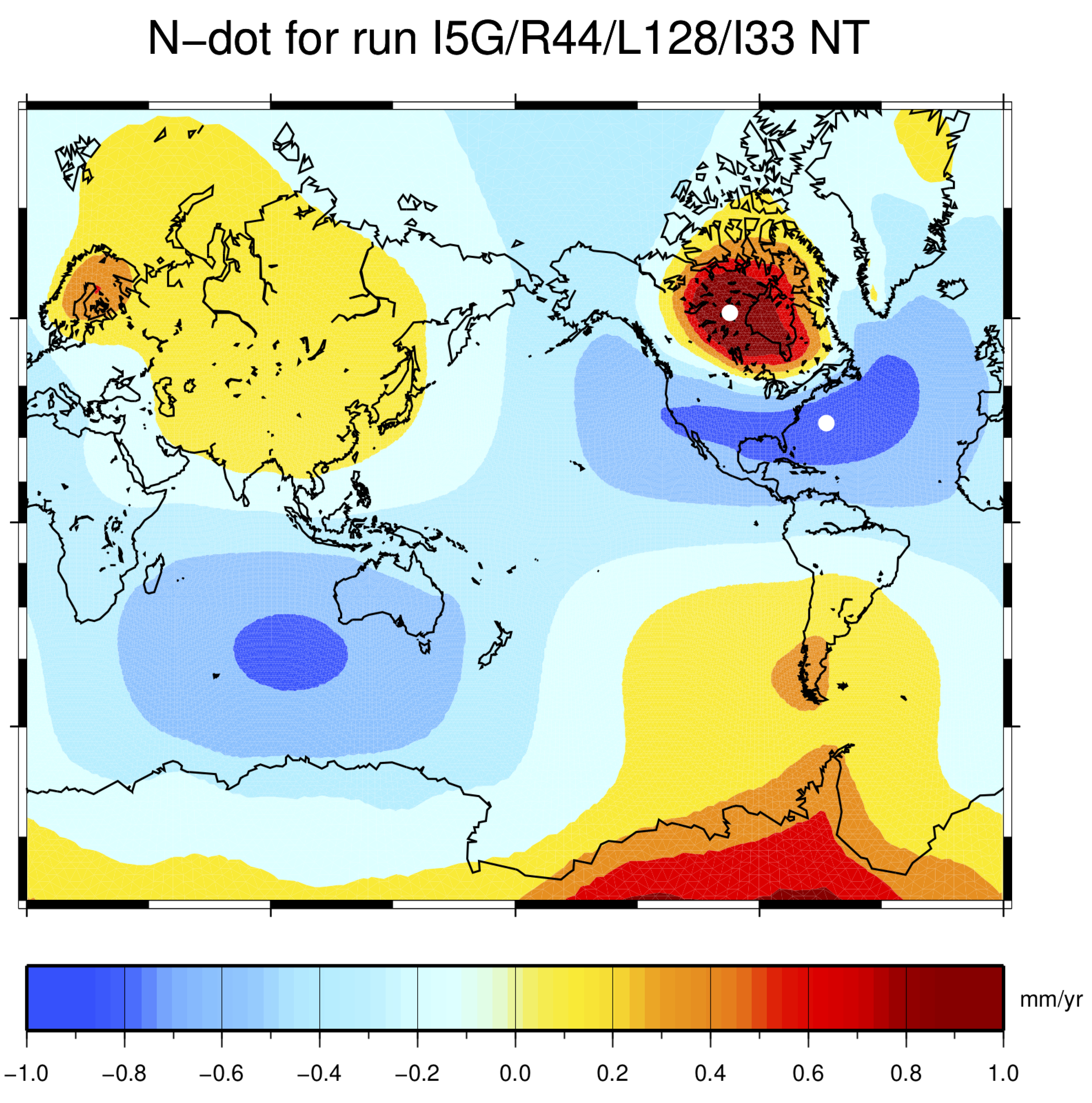
GIA fingerprint for the current rate of crustal uplift , according to our implementation of GIA model ICE-5G (VM2). The rates with largest absolute values, marked by white dots, are associated with the melting of the Laurentide ice sheet in north America and Canada, and are found in the same locations of Figure 3, with values of and mm year, respectively. The regional variability of the fingerprint appears to be comparable to that of in Figure 3 but the rotational lobes are much more developed.
Figure 4.
GIA fingerprint for the current rate of crustal uplift , according to our implementation of GIA model ICE-5G (VM2). The rates with largest absolute values, marked by white dots, are associated with the melting of the Laurentide ice sheet in north America and Canada, and are found in the same locations of Figure 3, with values of and mm year, respectively. The regional variability of the fingerprint appears to be comparable to that of in Figure 3 but the rotational lobes are much more developed.

Figure 5.
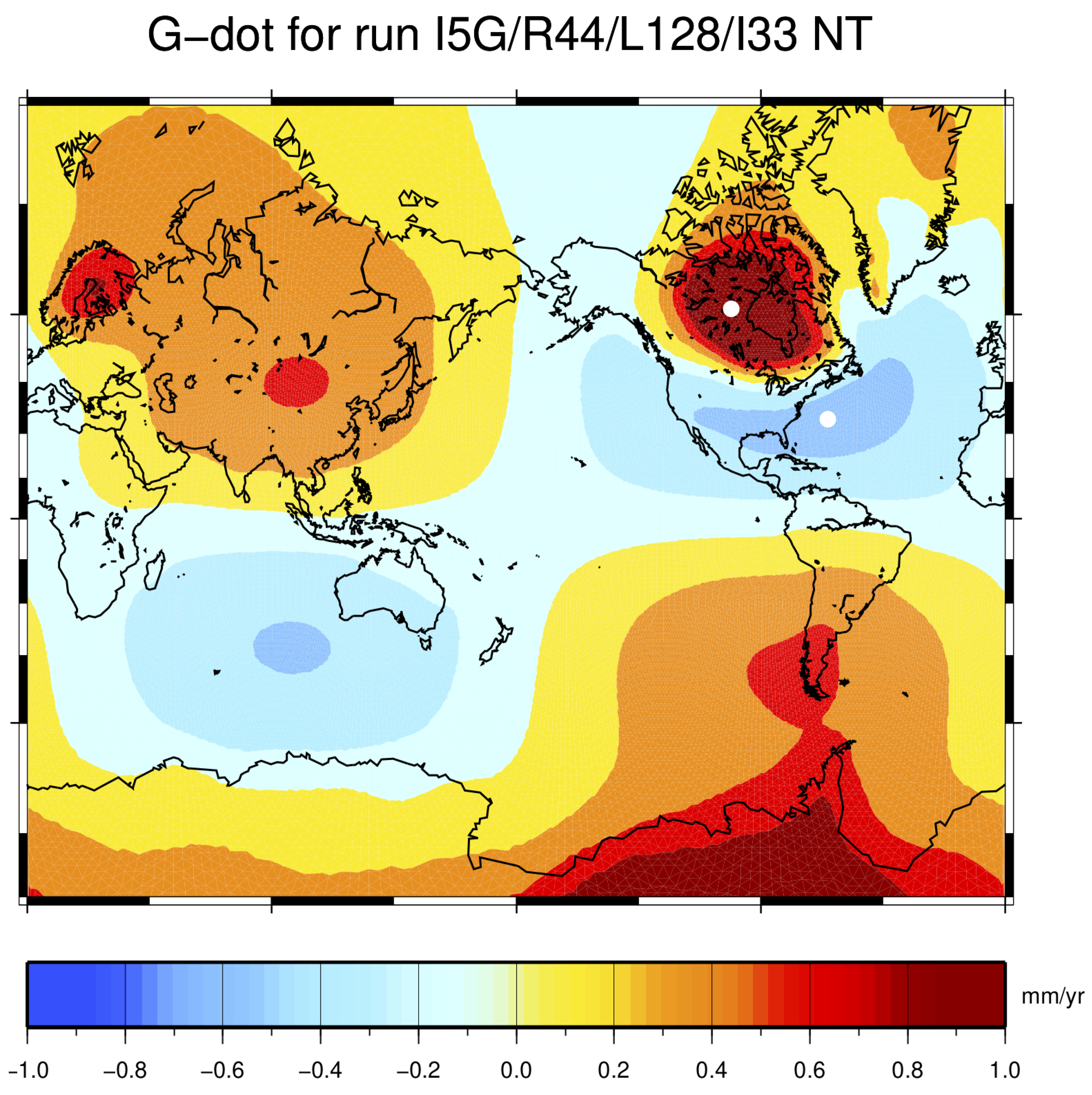
GIA fingerprint for i.e., the current rate of geoid height variation, according to our GIA simulation based upon model ICE-5G (VM2). The white dots show where the largest rates are predicted, with values of and mm year, respectively. The regional variability in this map, i.e., the alternation of local minima and maxima, is drastically reduced in comparison with and , giving to a very smooth semblance.
Figure 5.
GIA fingerprint for i.e., the current rate of geoid height variation, according to our GIA simulation based upon model ICE-5G (VM2). The white dots show where the largest rates are predicted, with values of and mm year, respectively. The regional variability in this map, i.e., the alternation of local minima and maxima, is drastically reduced in comparison with and , giving to a very smooth semblance.

Figure 6.
Fingerprint for , which represents the current rate of sea surface variation or absolute sea-level change according to our implementation of GIA model ICE-5G (VM2). White dots mark the places where the largest rates are expected, with and mm year, respectively. The spatial variability of matches that of in Figure 5, since the two fingerprints only differ by the spatially invariant term , where c is the FC76 constant.

Figure 7.
GIA fingerprint for the present-day rate of variation of the surface load , in units of mm year of water equivalent. The whole-Earth average is mm year to a very high precision. In oceanic areas, is strongly correlated with in Figure 3. In continental areas, only takes contributions in regions where, according to ICE-5G (VM2), ice thickness variations are still occurring or where the OF is still varying. These conditions are met in Greenland, where shows the extreme values (white dots), and in West Antarctica, respectively.


Table 1.
Values of density, rigidity and viscosity adopted in our realization of the rheological model VM2, with abbreviations LT, UM, TZ and LM denoting the lithosphere, the upper mantle, the transition zone and the lower mantle, respectively. With and we denote the radii of the base and of the top of each layer. A few spectral properties of this model are shown in Table 2.
| Radius, (km) | Radius, (km) | Density, (kg m−3) | Rigidity, (Pa × 1011) | Viscosity, (Pa·s × 1021) | Layer |
|---|---|---|---|---|---|
| 6281.000 | 6371.000 | 3192.800 | 0.596 | ∞ | LT |
| 6151.000 | 6281.000 | 3369.058 | 0.667 | 0.5 | UM1 |
| 5971.000 | 6151.000 | 3475.581 | 0.764 | 0.5 | UM2 |
| 5701.000 | 5971.000 | 3857.754 | 1.064 | 0.5 | TZ1 |
| 5401.000 | 5701.000 | 4446.251 | 1.702 | 2.7 | LM1 |
| 5072.933 | 5401.000 | 4615.829 | 1.912 | 2.7 | LM2 |
| 4716.800 | 5072.933 | 4813.845 | 2.124 | 2.7 | LM3 |
| 4332.600 | 4716.800 | 4997.859 | 2.325 | 2.7 | LM4 |
| 3920.333 | 4332.600 | 5202.004 | 2.554 | 2.7 | LM5 |
| 3480.000 | 3920.333 | 5408.573 | 2.794 | 2.7 | LM6 |
| 0 | 3480.000 | 10931.731 | 0 | 0 | Core |
Table 2.
Numerical values of the elastic (with superscript e) and fluid (with superscript f) loading Love numbers and for the rheological model VM2 (see Table 1), for some harmonic degrees l in the range . We use the compact notation and , where v is any value in the table and is an exponent. Note that, for this model, the elastic tidal Love numbers of degree are = while the fluid values are = .
| 2 | 4 | 16 | 64 | 128 | 256 | 512 | 1024 | ||
|---|---|---|---|---|---|---|---|---|---|
Table 3.
Ocean (top) and whole-Earth surface averages (bottom) of the present-day rate of change of GIA fingerprints considered in this study. In this table, the outputs of SELEN have been rounded to two significant figures. Although in the text we dwelt upon the new rotation theory (column (a)), results for the the traditional theory are also shown here in (b) while in (c) no rotational effects are taken into account. It is apparent that the spatial averages are only moderately affected by the choice of the rotation theory. The values of , and are numerically found to be < mm year in modulus. By virtue of mass conservation, their expected theoretical value should be exactly zero.
| Average | (a) New Theory (mm year−1) | (b) Traditional Theory (mm year−1) | (c) No Rotation (mm year−1) |
|---|---|---|---|
| −0.06 | −0.06 | −0.06 | |
| −0.27 | −0.30 | −0.24 | |
| −0.33 | −0.35 | −0.30 | |
| −0.06 | −0.09 | −0.04 | |
| +0.00 | +0.00 | +0.00 | |
| −0.27 | −0.27 | −0.26 | |
| +0.00 | +0.00 | +0.00 | |
| −0.27 | −0.27 | −0.26 | |
| +0.00 | +0.00 | +0.00 |
© 2019 by the authors. Licensee MDPI, Basel, Switzerland. This article is an open access article distributed under the terms and conditions of the Creative Commons Attribution (CC BY) license (http://creativecommons.org/licenses/by/4.0/).
Share and Cite
MDPI and ACS Style
Spada, G.; Melini, D. On Some Properties of the Glacial Isostatic Adjustment Fingerprints. Water 2019, 11, 1844. https://doi.org/10.3390/w11091844
AMA Style
Spada G, Melini D. On Some Properties of the Glacial Isostatic Adjustment Fingerprints. Water. 2019; 11(9):1844. https://doi.org/10.3390/w11091844
Chicago/Turabian StyleSpada, Giorgio, and Daniele Melini. 2019. "On Some Properties of the Glacial Isostatic Adjustment Fingerprints" Water 11, no. 9: 1844. https://doi.org/10.3390/w11091844
Note that from the first issue of 2016, this journal uses article numbers instead of page numbers. See further details here.