Application of an Analytic Methodology to Estimate the Movements of Moored Vessels Based on Forecast Data

Abstract

A port’s operating capacity and the economic performance of its concessions are intimately related to the quality of its operational conditions. This paper presents an analytical methodology for estimating the movements of a moored vessel based on field measurements and forecast data, specifically including ship dimensions and meteorological and maritime conditions. The methodology was tested and validated in the Outer Port of Punta Langosteira, A Coruña, Spain. It was determined that the significant wave height outside the port, and the ratio of the vessel’s length divided by its beam (L/B), are the variables that most influence movements. Furthermore, heave and surge are the movements with a better value of the coefficient of determination (R² values of 0.71 and 0.67, respectively), the sway (R² = 0.30) and roll (R² = 0.27) being the worst when using the available forecast variables of the Outer Port of Punta Langosteira. Despite their low R² values, sway and roll models are able to estimate the main trends of these movements. The obtained estimators provide good predictions with assumable error values (root mean square error—RMSE and mean absolute error—MAE), showing their potential application as a predictive tool. Finally, as a consequence, the A Coruña Port Authority has included the results of the methodology in its port management system allowing them to predict moored vessel behavior in the port.

1. Introduction and Objectives

In one respect, the quality of port operations can be defined by the maxim “the better a vessel’s stay in port, the greater the economic returns”. An important aspect that affects this process is the movements of the moored vessels. These movements are divided into three rotations (roll, pitch, and yaw) and three linear displacements (heave, surge, and sway). Each of these degrees of freedom is dependent on many variables, including climatic conditions, the vessel load cargo configuration, the vessel type, its location in the dock, the available defenses (fenders, bollards, etc.), and the mooring system employed [1].

On the other hand, decisions relating to the number of mooring lines, the ropes material (steel wire, synthetic fiber ropes, etc.), and the mooring arrangement depend on harbor pilot considerations, the mooring service providers, the mooring equipment on the berths, and the vessel captain. Finally, the vessel’s cargo configuration during operations modifies its center of gravity. This variation is difficult to ascertain with precision and would require a continuous record [2].

At present, there are a number of general recommendations regarding threshold values for movements during vessel loading and unloading operations [3,4]. Although these regulations establish movement criteria for safe working conditions, they do not clearly specify what type of statistical value of the movement they refer to (maximum, average or significant motion amplitudes). Moreover, because they are general recommendations, their specific application to each individual port requires a separate study [5].

Studies relating to operational capacity are traditionally conducted using three methodologies: numerical models, physical models, and field campaigns. Small-scale physical models [6,7,8] allow the simplified reproduction of port characteristics, vessel dimensions, mooring configuration, and different climatic conditions, but do not permit the accurate analysis of the variation in cargo configuration which occurs during operations. In addition, for a physical model to be reliable, it is important to assure that the model is accurate and realistic, which is achieved by costly construction and intense calibration [9,10]. On the other hand, although the advancement of numerical models facilitates the analysis of the behavior of a moored vessel and the influence on it of the mooring configurations or the effect of passing ships with lower computational and economic costs [11,12,13], these tools also have similar limitations as the physical models, such as the disadvantage of not reproducing the variations experienced by the position of the vessel’s center of gravity during the cargo operation. Therefore, using these two methodologies it is possible to analyze a specific loading condition (ship fully loaded, ballasted, etc.) but not the continuous variation of the same. Finally, studies conducted through field campaigns allow a comprehensive analysis of this process and its influence on the dynamic behavior of moored vessels. However, the current measurement techniques and data processing technology have limitations in terms of accuracy, the resolution of the instrumentation, temporary data logging, information storage, and computational cost. Nevertheless, at present there are studies in which some of the degrees of freedom are analyzed, together with the equations that define them and the loads that moored vessels are subjected to in specific situations, such as the swell generated by a vessel navigating in the port [14,15].

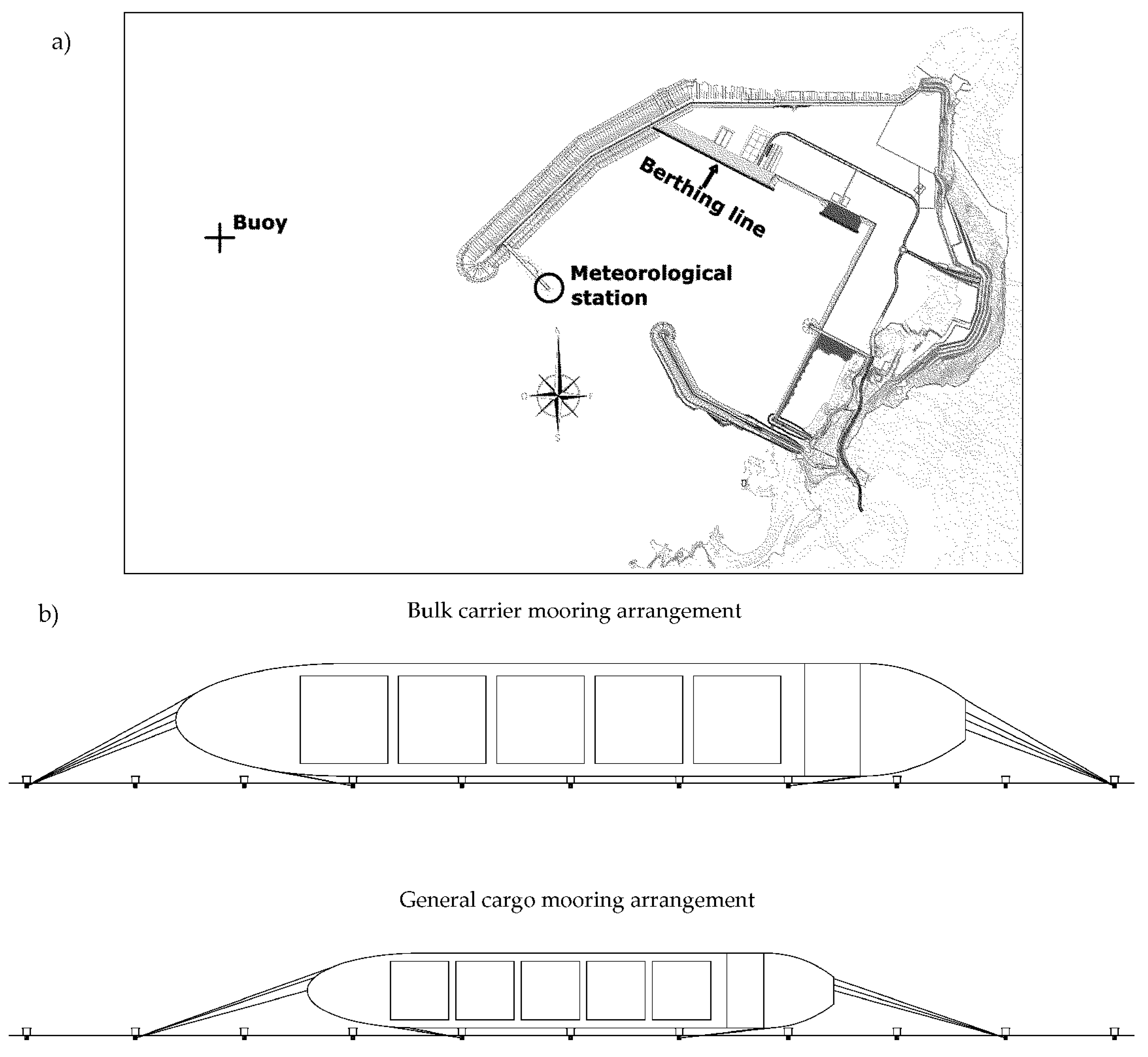
The objective of the present work was the development of an analytical methodology to predict the movements of moored vessels based on the data available by the Port Authority forecast and the vessel movements measured in a field campaign. This methodology has been applied and validated at the facilities of the Outer Port of Punta Langosteira, in A Coruña, Spain (Figure 1a). Each of the degrees of freedom was correlated to climatic variables and vessel dimensions, by means of multivariate linear approximation (transfer functions). These results allowed the A Coruña Port Authority to develop a management system to determine the port’s operating capacity, based on forecast data. With this system, it will be possible to evaluate the quality of the port’s operational facilities, determine the ideal working windows, and optimize the use of the port’s spaces. Furthermore, this methodology could be exportable to other ports if an analysis of the influential and available forecast variables is made, as well as a record of the movements of the moored vessels. Despite the influence of mooring lines on the behavior of vessels at berth, the mooring system information (material, initial pretension, and mooring arrangement) was not introduced as a variable to obtain the transfer functions, since no forecast data on these parameters would be available to subsequently feed the obtained models. In addition, as a results of the characteristics and layout of the port mooring equipment, vessels use two mooring arrangements (Figure 1b): 4-2-2-4 for large bulk carriers (4 bow lines–2 bow spring–2 stern springs–4 stern lines) and 3-2-2-3 for general cargo ships (3 bow lines–2 bow spring–2 stern springs–3 stern lines). Therefore, there is no variability in the number of moorings lines within the same vessel type.

2. Field Campaign and Forecast Data

Three field campaigns were conducted at the facilities of the Outer Port of Punta Langosteira in A Coruña for the measurement of the variables involved, lasting a total of 18 months (October–March 2015–2016, 2016–2017, and 2017–2018). The port is located 10 km southeast of the city of A Coruña in Spain and is protected by a 3360 m-long main breakwater and a spur breakwater 1320 m long. The current berthing line is 914 m long with an average depth of 22 m. The orientation of the dock is N62.7W and reaches a crest height 6.5 m above the zero datum of the port. A set of bollards spaced 31 m apart with a load capacity of 200 t is situated 0.75 m from the dock. In addition, there is a double-fender system protected by a shield to streamline vessel operations.

In order to compute the transfer functions, the six degrees of freedom of 27 vessels (15 Bulk carriers and 12 General cargo vessels) were recorded under different climatic conditions (

Table 1. Characteristics of the vessels measured during the field campaign.

Vessel	Type	Deadweight Tonnage DWT (t)	Length (m)	Beam (m)
Fu Da	Bulk carrier	71,330	224.9	32.2
Avax	Bulk carrier	87,030	225.0	32.2
Yannis	Bulk carrier	50,792	189.9	32.2
Western Boheme	Bulk carrier	37,000	186.9	28.6
Pina Cafiero	Bulk carrier	75,668	225.0	32.2
Jing Jin Hai	Bulk carrier	77,872	225.0	32.2
Lowlands Saguenay	Bulk carrier	37,152	179.9	30.0
Aloe	Bulk carrier	30,618	178.7	28.0
CSK Unity	Bulk carrier	77,105	225.0	32.2
Topaz	Bulk carrier	75,499	225.0	32.2
Walsall	Bulk carrier	58,018	189.9	32.3
Kyzicos	Bulk carrier	92,598	229.5	36.9
Nautical Lucia	Bulk carrier	63,548	199.9	32.2
Nord Saturn	Bulk carrier	77,288	225.0	32.2
Orange Harmony	Bulk carrier	81,837	229.0	32.2
Marc	General cargo	4135	89.8	13.6
Celine	General cargo	8600	129.4	15.8
Dominica	General cargo	13,022	127.3	21.2
Kelly C	General cargo	6250	106.0	15.5
Notos	General cargo	8049	125.1	16.4
Don Juan	General cargo	21,057	158.0	23.0
Eems River	General cargo	4066	89.9	12.5
Linau	General cargo	3699	88.0	12.8
Fortune	General cargo	12,692	138.9	21.3
Moraime	General cargo	7300	118.0	16.5
Onego Capri	General cargo	10,273	138.9	15.9
Oppland	General cargo	9273	107.0	18.4

). These vessels were located along the entire berthing line and represent a typical harbor fleet in this port.

The methodology used for the measurement of the movements was validated in other studies by the authors of this paper [16]. The measurement equipment consists of three systems that continuously record each of the vessel’s degrees of freedom with a frequency of 1 Hz. The first of these systems is an inertial measurement unit (IMU) [17] consisting of three accelerometers and three gyroscopes that record the roll and the pitch (Figure 2, Left). The second system comprises two electronic distance-measuring lasers for the sway and yaw measurements (Figure 2, Right). Finally, photogrammetric techniques were employed to measure the heave and surge movements [18] (Figure 2, Center).

The climatic variables were measured using the available instrumentation in the Spanish Port Authority network and the A Coruña Port Authority. The location of the instruments is shown in Figure 1. This decision was made since the port’s own meteorological forecasting system collects data at these points. In first place, the hydrodynamic variables were measured at the outer buoy of the Port of Punta Langosteira, located at 43°20′58.34″ N–8°33′41.32″ W at a depth of 60 m. During the first 20 min of each hour it recorded the following variables: significant wave height (H_s (m)), maximum wave height (H_max (m)), peak wave period (T_p (s)), average wave period (T_m (s)), and wave direction (Dir_W (°)). Second, the weather station located near the roundhead of the main breakwater was used to record wind speed and direction. The instrumentation continuously records the average wind speed (V_w (km/h)), wind gust speed (V_g (km/h)), average direction, and wind gust direction (Dir_Vw (°) and Dir_Vg (°)). However, the port weather forecast system only provides 72 h in advance data of the variables H_s (m), T_p (s), and Dir_W (°) at the buoy location, and, V_w (km/h) and Dir_Vw (°) at the weather station, so these variables were finally used in this study. This forecasting system was developed by the Spanish government agency Puertos del Estado in collaboration with the State Meteorological Agency (AEMET). This system is driven by wind fields supplied by AEMET from the High Resolution Limited Area Model (HIRLAM). The system starts a new execution twice a day providing data outputs with a time resolution of 1 h. To ensure good initial conditions, before the forecast starts, the model is forced using wind analyzed fields of the 12 h prior to forecast initialization [19].

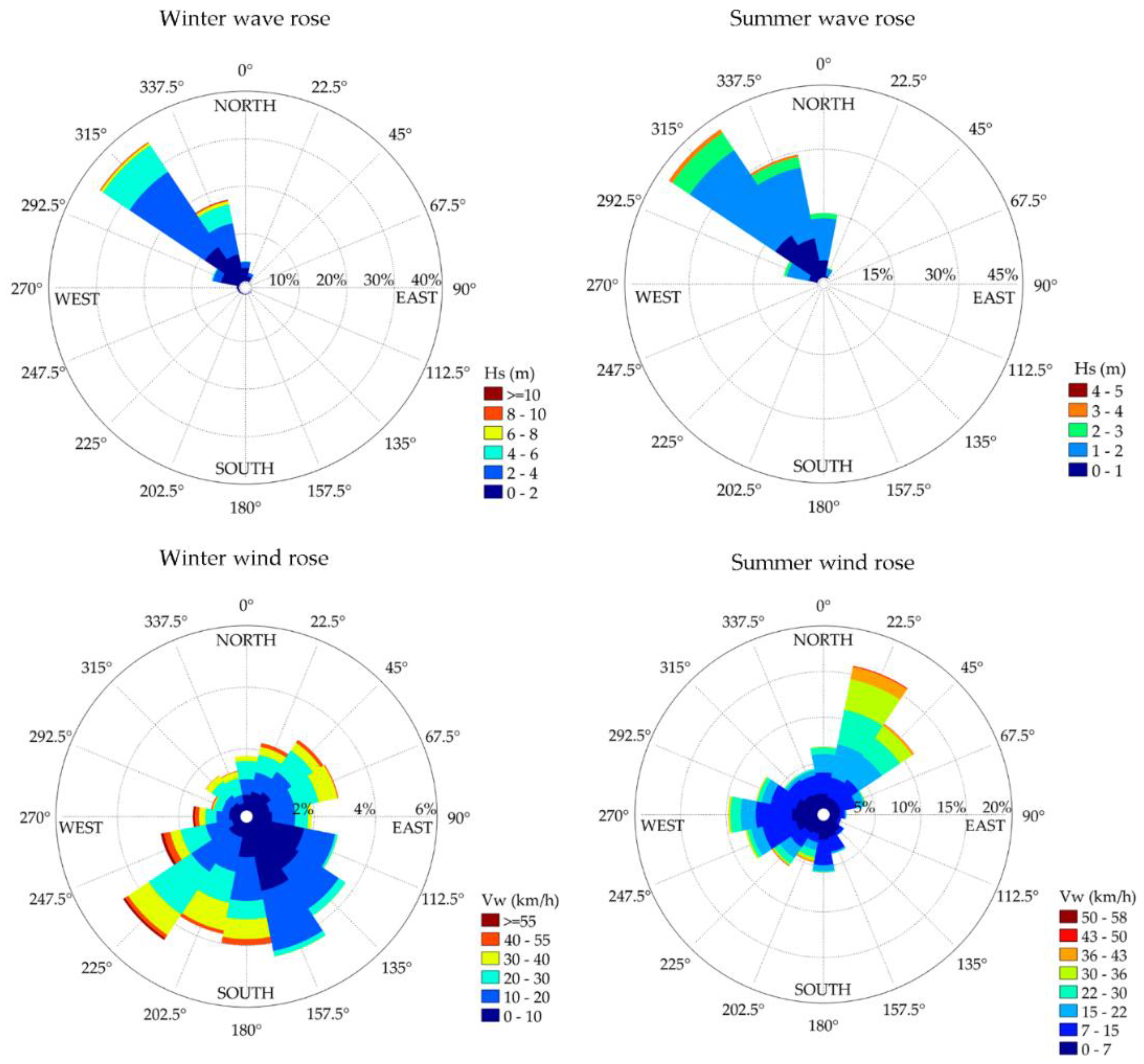
The seasonal wind and wave roses (winter and summer) at the buoy position for the period 2015–2018 are shown in Figure 3, in order to clarify the values of the main forcings acting in the Outer Port of Punta Langosteira.

Although the models for estimating the movements of moored vessels were obtained with observational meteorological and ocean data (recorded by the wave buoy and the weather station), they are run with forecast data. Therefore, it is important to know the differences between both sources of information (observational data vs. forecast data). To this end, an analysis of the estimation errors of each variable (H_s (m), T_p (s), Dir_w (°), V_w (km/h), and Dir_Vw (°)) was conducted.

Table 2. Coefficient of determination (R²), root mean square error (RMSE) and mean absolute error (MAE) of forecast and observed meteorological and ocean variables.

Forecast Variable vs. Observed Variable	R2	RMSE	MAE
Hs (m) forecast vs. Hs (m) observed	0.86	0.39 m	0.29 m
Tp (s) forecast vs. Tp (s) observed	0.63	1.9 s	1.2 s
Dirw (°) forecast vs. Dirw (°) observed	0.77	18.2°	11.3°
Vw (km/h) forecast vs. Vw (km/h) observed	0.64	6.8 km/h	5.2 km/h
DirVw (°) forecast vs. DirVw (°) observed	0.51	55.1°	36.5°

shows the obtained results.

On the one hand, H_s (m), T_p (s), Dir_w (°), and V_w (km/h) variables present a better approximation to the observed value, showing acceptable prediction errors (MAE values of 0.29 m, 1.2 s, 11.3°, and 5.2 km/h, respectively). On the other hand, Dir_Vw (°) shows the largest deviation between the observed and the forecast value (MAE value of 36.5°). Since the models are fed with forecast data, having an accurate weather forecasting system will provide similar results in terms of accuracy to those obtained by these models in their development stage.

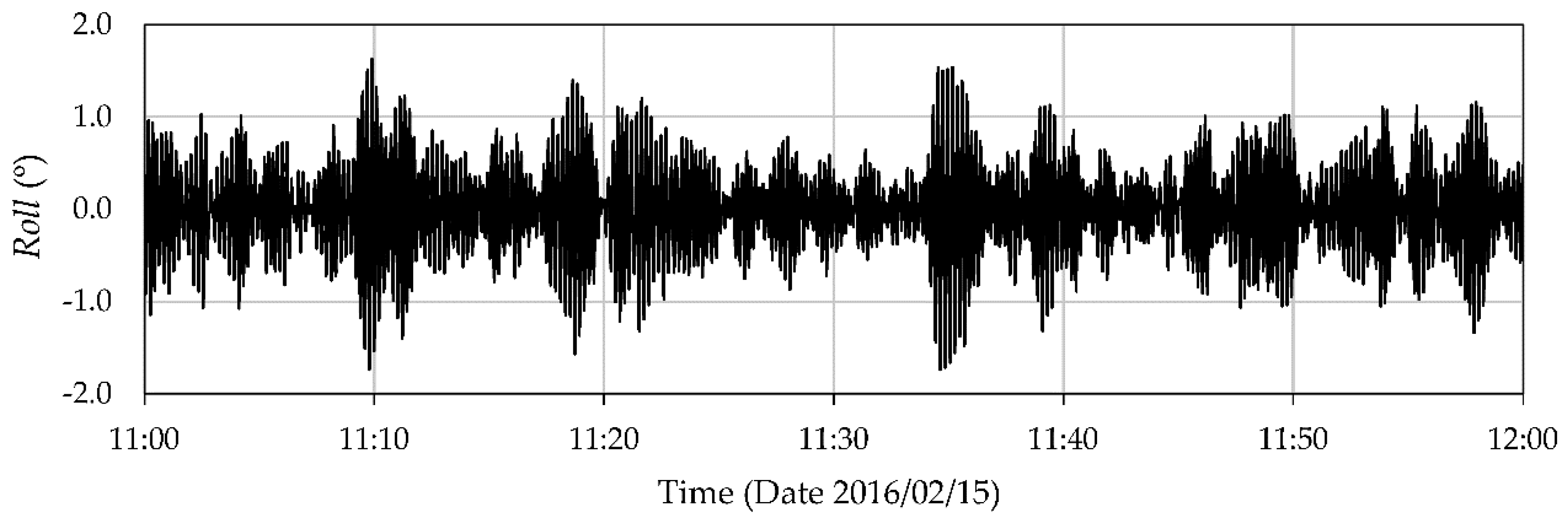
As previously mentioned, the wave buoy employed in this study characterizes the main ocean variables of each sea state (1-h duration) using the records obtained during the first 20 min of each hour. For this reason, the joint analysis of the data was carried out using only the concomitant data of both wind, waves, and vessel movements. Regarding moored vessels behavior, the analysis of motion time series was based on a zero crossing technique. A peak-to-peak criterion was applied to each movement to obtain their amplitudes, except in the case of sway motion, for which the zero-peak criterion was used. Complete time series of each motion were split into blocks of 1-h duration, obtaining the maximum motion amplitude, average motion amplitude, and significant motion amplitude calculated as the average of the highest third for each block [16]. 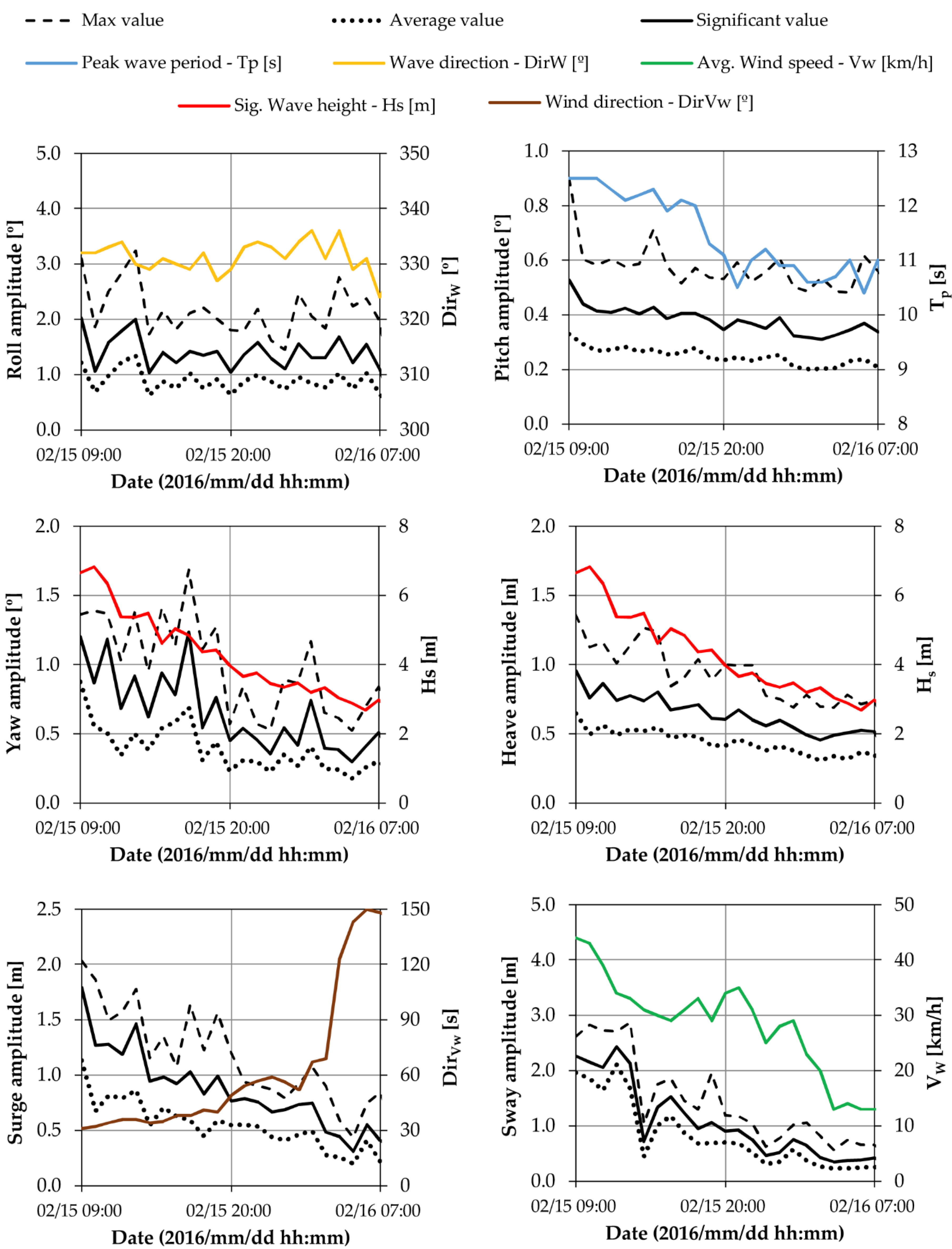Figure 4 shows a sample of roll motion time series recorded on the bulk carrier vessel WESTERN BOHEME. The analysis of the maximum, average, and significant amplitudes of each motion and their concomitant climatic forcings recorded on the same vessel are shown in Figure 5.

As can be seen in Figure 5, a moored ship that under specific meteorological and ocean conditions moves with certain amplitudes may experience a maximum punctual movement much larger than its significant or average movement. This value that stands out from the main trend of the movement could be occasionally caused by the action of other external agents such as the waves generated by passing vessels or the punctual modification of the mooring lines tension to adapt them to the tidal variations.

3. Analytic Methodology

This section presents the analytical methodology developed in this study for the calculation of each of the transfer functions. The analysis was performed for significant movements. This parameter has commonly been used in similar studies to evaluate the dynamic behavior of a moored vessel during its stay in port [16,20,21]. Also, the use of the significant value assures that motions and wave parameters (significant wave height and peak wave period) are obtained following the same statistical analysis. This can contribute to achieving better relations with the main forcings of moored vessels’ behavior. In addition, the range and independence of each of the variables used were also calculated.

3.1. Dataset Creation

First, a dataset was created to handle the calculation of the transfer functions. The range of validity is shown in

Table 3. Range of the variables considered for the calculation of the transfer functions.

Range	Length (m)	Beam (m)	Hs (m)	DirW (°)	Tp (s)	Vw (km/h)	DirVw (°)
Min.	88.0	12.5	1.04	1.0	5.5	0.1	4.0
Max.	229.5	36.9	8.95	359	18.2	80.0	351.0

Abbreviations: H_s (m)—Significant wave height; Dir_W (°)—Wave direction; T_p (s)—Peak wave period; V_w (km/h)—Average wind speed; Dir_Vw (°)—Wind direction.

and defines the values of each of the variables recommended for the equations calculated in this study.

The homogeneity in the distribution of variables of the dataset was analyzed. To this end, each data of a given variable was dimensionalized with the highest value of the same (Variable value (i)/Maximum variable value). In this way, the spectrum of values was contained between 0 and 1. Figure 6 shows the cumulative frequency of each parameter (Y-axis) within its range (X-axis). Therefore, in a situation of homogeneous distribution of the data, the plot would correspond with the bisector of the graph.

The results show that the significant wave height (Hs (m)) and wind velocity (V_W (km/h)) variables are concentrated between 0.1 and 0.4 of their range. The wind direction (Dir_Vw (°)) presents a homogeneous distribution in its range. However, the variables representing the peak wave period (T_p (s)), wave direction (Dir_w (°)), length (m), and beam (B [m]), are all concentrated between 0.6 and 1 for the majority of the data. With the aim of more precisely quantifying the variables without dimensionalizing them,

Table 4. Frequency of the data recorded during the field campaign for each of the variables.

Hs (m)		Tp (s)		DirW (°)		Vw (km/h)		DirVw (°)		Length (m)		Beam (m)
Range	%	Range	%	Range	%	Range	%	Range	%	Range	%	Range	%
<1.0	0%	<4	0%	N [337.5–22.5]	16%	0–10	14%	N [337.5–22.5]	2%	<100	1%	<10	0%
1–2	27%	4–6	0%	NE [22.5–67.5]	0%	10–20	35%	NE [22.5–67.5]	27%	100–150	13%	10–15	1%
2–3	37%	6–8	2%	E [67.5–112.5]	0%	20–30	24%	E [67.5–112.5]	4%	150–200	27%	15–20	9%
3–4	19%	8–10	19%	SE [112.5–157.5]	0%	30–40	16%	SE [112.5–157.5]	19%	200–250	59%	20–25	6%
4–5	8%	10–12	38%	S [157.5–202.5]	0%	40–50	7%	S [157.5–202.5]	8%	>250	0%	25–30	13%
5–6	7%	12–14	21%	SW [202.5–247.5]	0%	50–60	3%	SW [202.5–247.5]	19%			>30	70%
6–7	1%	14–16	15%	W [247.5–292.5]	2%	60–70	1%	W [247.5–292.5]	14%
7–8	1%	16–18	4%	NW [292.5–337.5]	81%	>70	0%	NW [292.5–337.5]	6%
8–9	1%	>18	1%
>9.0	0%

shows the frequency ranges and values for each of the variables.

An amount of 83% of the significant wave height data (Hs (m)) is concentrated in the range 1.0 ≤ H_s (m) ≤ 4. For the peak period, 93% of the data lies between 8 ≤ T_p (s) ≤ 16. Moreover, 38% of the data is concentrated within a 2-s range (10 s–12 s). Most of the data pertaining to the wave direction come from the NW direction (81%). Regarding the ship’s dimension, 59% of the length values and 70% of the beam values are for the largest vessels (200–250 m length and > 30 m beam). In view of the results it can be seen that some of the possible combinations between the variables are not defined by a very high number of data points.

3.2. Statistical Response, Variables and Predictors

Next, the analytical methodology employed, the variables used, and their influence on each of the degrees of freedom is presented.

The variables were selected taking their a priori possible influence on vessel movements into account. They were divided into three groups, depending on whether they were climatic variables, vessel dimensions, or dimensionless vessel size features. The latter were obtained by scaling the vessel size measurements with the following wave characteristics: significant wave height (H_s (m)), and wave length in deep water (L_op (m)).

Table 5. Response and predictor variables, with corresponding tags.

Movement (yi)	Name	Variables (Xm)	Name	Typology
Roll	y1	Wave height (Hs (m))	X1	Meteorological and ocean variables
Pitch	y2	Wave period (Tp (m))	X2
Heave	y3	Wave length (Lop (m))	X3
Surge	y4	Wave steepness (s)	X4
Sway	y5	Wave direction (DirW (°))	X5
Yaw	y6	Wind velocity (Vw (km/h))	X6
		Wind direction (DirVw (°))	X7
		Length (L (m))	X8	Vessel dimensions
		Beam (B (m))	X9
		Length/Beam (L/B)	X10	Dimensionless
		Length/Hs	X11
		Length/Lop	X12
		Beam/Hs	X13
		Beam/Lop	X14

shows the description of all the predictor and response (vessel movements) variables obtained, studied, and modeled in this work.

The transfer functions were calculated and analyzed using statistical correlation studies and multivariate linear regression techniques [22]. This methodology has recently been applied to various different engineering domains, including naval and oceanic engineering [23,24,25]. In the case of ocean engineering, following a similar methodology, Carral-Couce et al. [23] developed nonlinear and multivariate linear regression models to estimate the traction of towing and anchor-handling winches. Additionally, the transit time to cross the Panama Canal’s new locks was estimated using multivariate linear regression [24], and the effect of vessel dimensions, type, and fishing ground were also modeled to estimate net drum and winch traction for trawler design tasks [25]. These techniques were also used to forecast wave height [26] and vessel traffic flow [27], among various other applications. For the present case, the proposed multivariate regression model can be expressed as Equation (1):

$$y_i={\widehat{\beta }}_0+{\displaystyle \sum }_{m=1}^M{\widehat{\beta }}_m{x}_m+{\widehat{\epsilon }}_i, with i=1,2,\dots ,6 and m=1,2,\dots ,14$$

(1)

where $y_i$ represents the sample values of the response variable (vessel movement) corresponding to the multivariate linear model, $x_m$ represents the m predictor variables (there were up to M = 14 variables analyzed), and ${\widehat{\epsilon }}_i$ represents the model’s residuals or the discrepancy between the real $y_i$ and the model estimates, ${\widehat{y}}_i={\widehat{\beta }}_0+{{\displaystyle \sum }}_{m=1}^M{\widehat{\beta }}_m{x}_m$. The i index accounts for the vessel’s degrees of freedom (roll, pitch, heave, surge, sway, and yaw). ${\widehat{\beta }}_0$ represents the constant term of each model, and ${\widehat{\beta }}_m$ represents the model’s parameter estimates corresponding to each of the independent variables. They account for the linear effect of each predictor on the response.

4. Results and Discussion

This section includes the descriptive analysis, including the predictor correlation study, the multivariate linear model’s estimation, and the model’s predictions of vessel movements obtained from the previously described dataset.

4.1. Correlation Analysis

The predictors of a multivariate linear model should be uncorrelated in order to obtain reliable model parameter estimations, and, hence, accurate and precise predictions [23,24,25,28]. Indeed, the existence of multicollinearity leads to estimates of model parameters being highly dependent on sample data, preventing an analysis of the effect of each predictor or covariate on the response, and limiting the model’s ability to generate accurate predictions. Accordingly, a pairwise dependence relationship analysis should be performed prior to including the predictors in the final model [28]. The most widely used measurement for goodness of fit is the Pearson coefficient (r). At this point, it is important to note that the inclusion of new additional predictors to the model always increases the Pearson coefficient. Nevertheless, those predictors must be uncorrelated to prevent spurious dependence relationships and inaccurate models. Accordingly, the dependence structure of the predictors was analyzed by calculating the Pearson coefficient, r (

Table 6. Pairwise Pearson linear correlation coefficients for the predictors (in gray when r ≥ 0.6 or r < −0.6).

r
		Hs (m)	Tp (s)	Lop (m)	s	DirW (°)	Vw (km/h)	DirVw (°)	L (m)	B (m)	L/B	L/Hs	L/Lop	B/Hs	B/Lop
r	Hs (m)	1.0	0.3	0.3	0.7	0.1	0.3	0.1	−0.1	−0.1	0.1	−0.8	−0.3	−0.8	−0.3
	Tp (s)	0.3	1.0	1.0	−0.4	0.1	−0.1	−0.1	0.1	0.1	0.1	−0.2	−0.7	−0.2	−0.8
	Lop (m)	0.3	1.0	1.0	−0.4	0.1	−0.1	−0.1	0.1	0.1	0.1	−0.2	−0.7	−0.2	−0.7
	s	0.7	−0.4	−0.4	1.0	0.1	0.3	0.1	−0.1	−0.1	0.1	−0.6	0.4	−0.6	0.4
	DirW (°)	0.1	0.1	0.1	0.1	1.0	−0.1	0.1	0.1	0.1	0.0	0.0	0.0	0.0	0.0
	Vw (km/h)	0.3	−0.1	−0.1	0.3	−0.1	1.0	0.1	−0.1	0.0	−0.2	−0.3	0.0	−0.3	0.0
	DirVw (°)	0.1	−0.1	−0.1	0.1	0.1	0.1	1.0	−0.1	−0.1	−0.1	−0.1	0.0	−0.1	0.0
	L (m)	−0.1	0.1	0.1	−0.1	0.1	−0.1	−0.1	1.0	0.9	0.2	0.5	0.4	0.4	0.4
	B (m)	−0.1	0.1	0.1	−0.1	0.1	0.0	−0.1	0.9	1.0	0.0	0.5	0.4	0.5	0.4
	L/B	0.1	0.1	0.1	0.1	0.0	−0.2	−0.1	0.2	0.0	1.0	0.1	0.1	0.0	0.0
	L/Hs	−0.8	−0.2	−0.2	−0.6	0.0	−0.3	−0.1	0.5	0.5	0.1	1.0	0.4	1.0	0.4
	L/Lop	−0.3	−0.7	−0.7	0.4	0.0	0.0	0.0	0.4	0.4	0.1	0.4	1.0	0.4	1.0
	B/Hs	−0.8	−0.2	−0.2	−0.6	0.0	−0.3	−0.1	0.4	0.5	0.0	1.0	0.4	1.0	0.4
	B/Lop	−0.3	−0.8	−0.7	0.4	0.0	0.0	0.0	0.4	0.4	0.0	0.4	1.0	0.4	1.0

).

Table 6 shows that the wave period (T_p (s)) and wave length (L_op (m)) present a direct linear relationship (r = 1) due to their definition. In addition, the wave height (H_s (m)) and steepness (s) are also correlated (r > 0.6). Additionally, the vessel size predictors are also significantly correlated. This is the case for vessel length (L (m)) and beam (B (m)), which are very strongly correlated (r ≥ 0.9). A similar dependence structure is obtained when the size dimensionless predictor variables are studied. 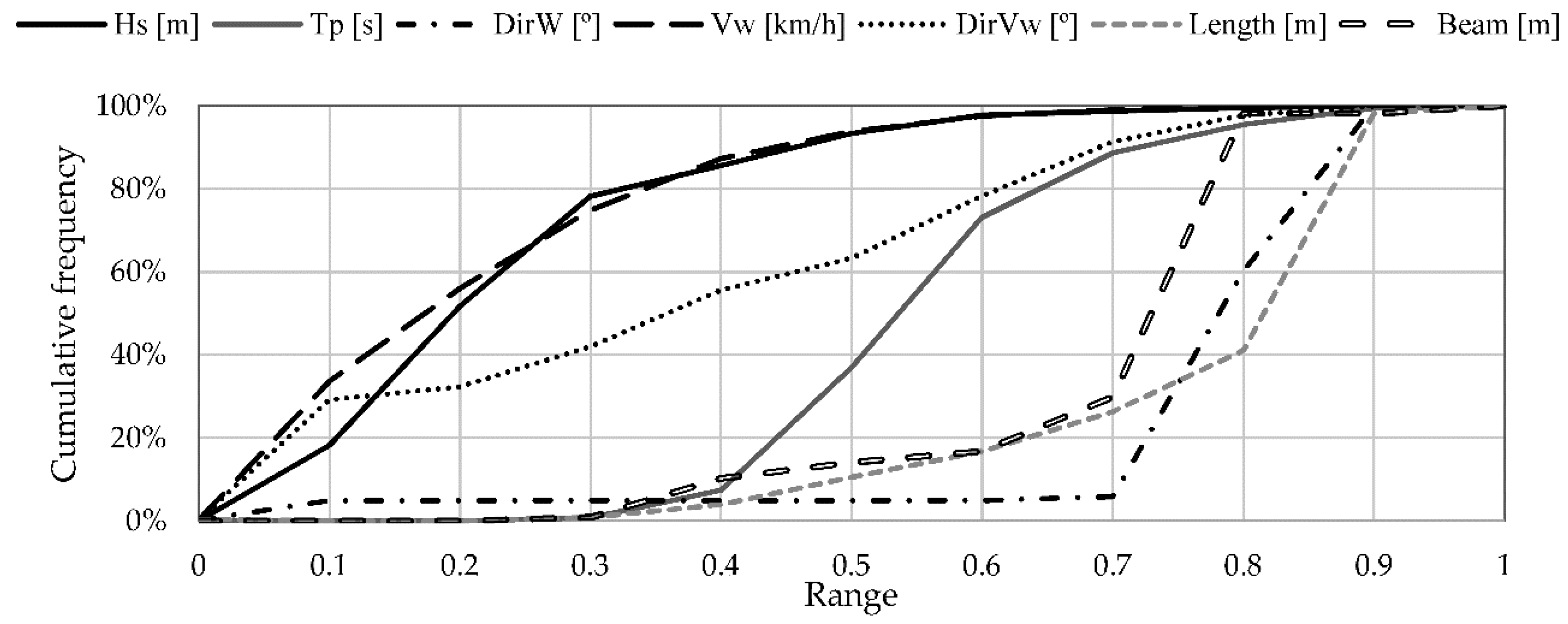Taking into account the fact that the dimensionless variables were derived from the vessel size and meteorological and ocean variables, Table 6 shows that they are strongly correlated with both size and meteorological and ocean predictors. On the other hand, it can be observed that the dimensionless variable Length/Beam is independent, and this allows the influence of the size of the vessel to be introduced into the analysis.

On the basis of the results depicted in Table 6, linear regression models were developed using variables that were independent of each other. Thus, these models were constructed using five hydrodynamic predictors (H_s (m), T_p (s), Dir_W (°), V_w (km/h), Dir_Vw (°)) and the dimensionless variable Length/Beam (

Table 7. Predictors involved in fitting regression models.

Selected Predictors
Wave height (Hs (m))
Wave period (Tp (s))
Wave direction (DirW (°))
Wind velocity (Vw (km/h))
Wind direction (DirVw (°))
Length/Beam (L/B)

).

The variables H_s (m) and T_p (s) were selected instead of s (wave steepness) and L_op (m) since they are the main parameters that define the characteristics of a sea state (together with Dir_W (°)). In addition, their values are directly provided by both the wave buoy and the weather forecasting system of the Port, facilitating the data acquisition and the implementation of the models. Regarding vessel dimensions, neither L (m) nor B (m) was selected to participate as an independent variable since their information was already included in the dimensionless variable L/B.

4.2. Regression Modelling of Vessel Movements

Once the variables that could potentially participate in the generation of the models were selected, the next step consisted in identifying those that had an important influence on the prediction provided by each model. To this end, an Akaike criterion (AIC) was used [29]. First, the multivariate linear regression models were calculated including all selected predictors. The parameters corresponding to each predictor, ${\widehat{\beta }}_m$ were estimated from the data base by means of the least squares method. Then, a statistical significance analysis of each variable was carried out, selecting those with a level of significance α ≤ 0.01 (

Table 8. Summary of the selected predictors for each response variable. Variables that have an effect on the response significantly different from zero are indicated by a cross (significance level α ≤ 0.01).

	Roll (y1)	Pitch (y2)	Heave (y3)	Surge (y4)	Sway (y5)	Yaw (y6)
Hs	x	x	x	x	x	x
Tp	x	x			x
DirW	x		x	x		x
Vw	x		x		x
DirVw				x	x
L/B	x	x	x	x	x	x

).

Finally, models were re-calculated using only the most influential predictors in each vessel movement, obtained from the significance analysis (Table 8). Adopting this methodology ensured that the models would provide predictive results. The following expressions show the structure and selected variables for each transfer function:

$${\mathrm{y}}_1 \left(\mathrm{Roll}\right)={ \mathsf{\beta }}_{0_{\mathrm{Roll}}}+{\mathsf{\beta }}_{1_{{\mathrm{H}}_{\mathrm{s}}}}·{\mathrm{H}}_{\mathrm{s}}+{\mathsf{\beta }}_{1_{{\mathrm{T}}_{\mathrm{p}}}}·{\mathrm{T}}_{\mathrm{p}}+{\mathsf{\beta }}_{1_{{\mathrm{Dir}}_{\mathrm{W}}}}·{\mathrm{Dir}}_{\mathrm{W}}+{\mathsf{\beta }}_{1_{{\mathrm{V}}_{\mathrm{W}}}}·{\mathrm{V}}_{\mathrm{W}}+{\mathsf{\beta }}_{1_{\frac{\mathrm{L}}{\mathrm{B}}}}·\frac{\mathrm{L}}{\mathrm{B}}$$

(2)

$${\mathrm{y}}_2 \left(\mathrm{Pitch}\right)={ \mathsf{\beta }}_{0_{\mathrm{Pitch}}}+{\mathsf{\beta }}_{2_{{\mathrm{H}}_{\mathrm{s}}}}·{\mathrm{H}}_{\mathrm{s}}+{\mathsf{\beta }}_{2_{{\mathrm{T}}_{\mathrm{p}}}}·{\mathrm{T}}_{\mathrm{p}}+{\mathsf{\beta }}_{2_{\frac{\mathrm{L}}{\mathrm{B}}}}·\frac{\mathrm{L}}{\mathrm{B}}$$

(3)

$${\mathrm{y}}_3 \left(\mathrm{Heave}\right)={ \mathsf{\beta }}_{0_{\mathrm{Heave}}}+{\mathsf{\beta }}_{3_{{\mathrm{H}}_{\mathrm{s}}}}·{\mathrm{H}}_{\mathrm{s}}+{\mathsf{\beta }}_{3_{{\mathrm{Dir}}_{\mathrm{W}}}}·{\mathrm{Dir}}_{\mathrm{W}}+{\mathsf{\beta }}_{3_{{\mathrm{V}}_{\mathrm{W}}}}·{\mathrm{V}}_{\mathrm{W}}+{\mathsf{\beta }}_{3_{\frac{\mathrm{L}}{\mathrm{B}}}}·\frac{\mathrm{L}}{\mathrm{B}}$$

(4)

$${\mathrm{y}}_4 \left(\mathrm{Surge}\right)={ \mathsf{\beta }}_{0_{\mathrm{Surge}}}+{\mathsf{\beta }}_{4_{{\mathrm{H}}_{\mathrm{s}}}}·{\mathrm{H}}_{\mathrm{s}}+{\mathsf{\beta }}_{4_{{\mathrm{Dir}}_{\mathrm{W}}}}·{\mathrm{Dir}}_{\mathrm{W}}+{\mathsf{\beta }}_{4_{{\mathrm{Dir}}_{{\mathrm{V}}_{\mathrm{W}}}}}·{\mathrm{Dir}}_{{\mathrm{V}}_{\mathrm{W}}}+{\mathsf{\beta }}_{4_{\frac{\mathrm{L}}{\mathrm{B}}}}·\frac{\mathrm{L}}{\mathrm{B}}$$

(5)

$${\mathrm{y}}_5 \left(\mathrm{Sway}\right)={ \mathsf{\beta }}_{0_{\mathrm{Sway}}}+{\mathsf{\beta }}_{5_{{\mathrm{H}}_{\mathrm{s}}}}·{\mathrm{H}}_{\mathrm{s}}+{\mathsf{\beta }}_{5_{{\mathrm{T}}_{\mathrm{p}}}}·{\mathrm{T}}_{\mathrm{p}}+{\mathsf{\beta }}_{5_{{\mathrm{V}}_{\mathrm{W}}}}·{\mathrm{V}}_{\mathrm{W}}+{\mathsf{\beta }}_{5_{{\mathrm{Dir}}_{{\mathrm{V}}_{\mathrm{W}}}}}·{\mathrm{Dir}}_{{\mathrm{V}}_{\mathrm{W}}}+{\mathsf{\beta }}_{5_{\frac{\mathrm{L}}{\mathrm{B}}}}·\frac{\mathrm{L}}{\mathrm{B}}$$

(6)

$${\mathrm{y}}_6 \left(\mathrm{Yaw}\right)={ \mathsf{\beta }}_{0_{\mathrm{Yaw}}}+{\mathsf{\beta }}_{6_{{\mathrm{H}}_{\mathrm{s}}}}·{\mathrm{H}}_{\mathrm{s}}+{\mathsf{\beta }}_{6_{{\mathrm{Dir}}_{\mathrm{W}}}}·{\mathrm{Dir}}_{\mathrm{W}}+{\mathsf{\beta }}_{6_{\frac{\mathrm{L}}{\mathrm{B}}}}·\frac{\mathrm{L}}{\mathrm{B}}$$

(7)

Each multivariate linear regression model was adjusted with 80% of the composed data sample. The rest of the data was reserved for external validation of the transfer functions calculated by the models.

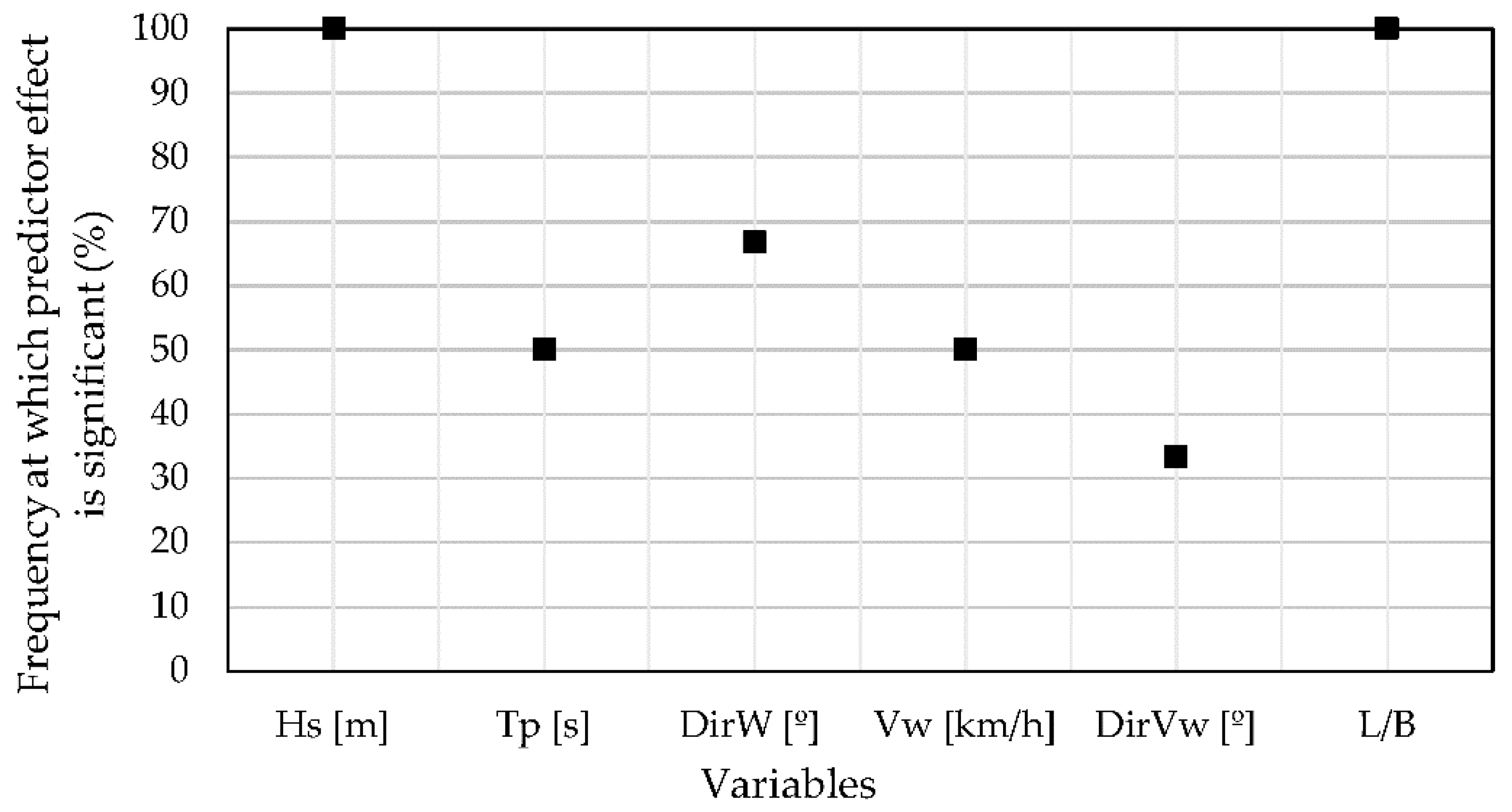
In order to quantify the importance of each variable for vessel movements, a relative frequency descriptive analysis was performed (Figure 7). From this analysis, the wave height (H_s (m)) and the dimensionless variable Length/Beam (L/B) effect on the response was found to be significant in all (100%) of the regression models performed (transfer functions), while the wave direction (Dir_W (°)). effect was non-zero in 66.67% of the transfer functions performed. In addition, the wave period (T_p (s)) and wind velocity (V_w (km/h)) were significant in 50% of the movements. Finally, wind direction (Dir_Vw (°)) effect was only significant for surge and sway movements.

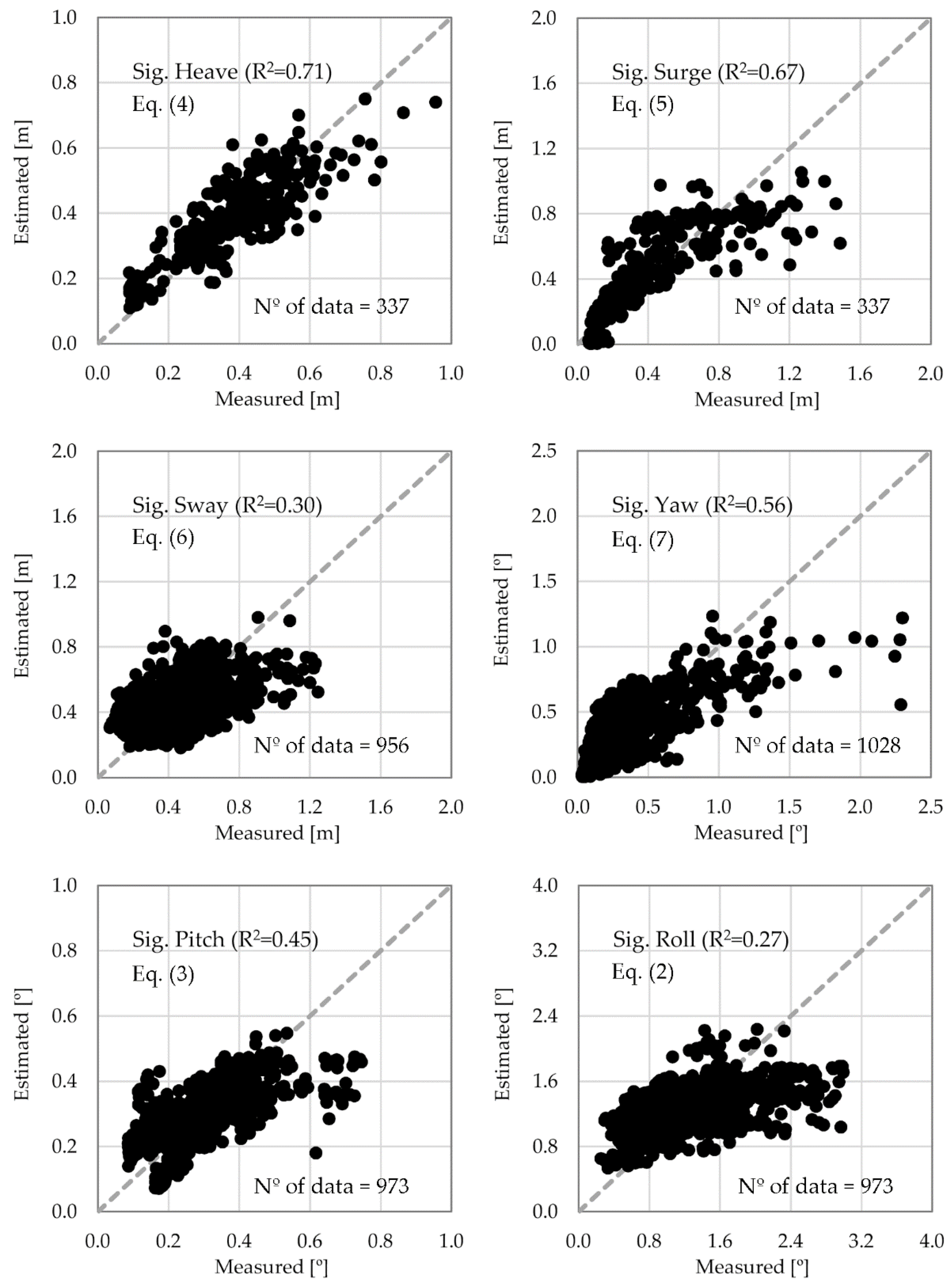
Figure 8 shows the results obtained with each of the models constructed. This data visualization provides information about the goodness of fit, the ability to predict vessel movements using a variable-dependent model, and the model’s accuracy and precision.

As can be observed, the models with the highest accuracy and precision were those that estimate the heave and the surge. This trend was also observed for the yaw and pitch movements. The lowest accuracy was obtained for the sway and the roll. These two movements had greater variability over time, as well as an inertial component from the vessel and the cargo, so their accuracies were lower. Accordingly, the fittings for these latter vessel movements were less precise (a greater dispersion of points around the diagonal). However, although these models did not allow the real motion amplitude to be predicted accurately, they were able to estimate the main trends of these movements.

In addition, the R² coefficients and the root mean square error (RMSE) provided a quantitative measure of each model’s goodness of fit (

Table 9. Values of the R² coefficient and the root mean square error (RMSE) of the calculated transfer functions.

Movement	R2	RMSE
Heave	0.71	0.08 m
Surge	0.67	0.18 m
Sway	0.30	0.18 m
Yaw	0.56	0.21°
Pitch	0.45	0.09°
Roll	0.27	0.46°

). The best goodness of fit was produced for the heave movement, with an R² value of 0.71 and an RMSE of 0.08 m.

The surge movements fitted with R² = 0.67, while the yaw and pitch movements had R² values of 0.56 and 0.45, respectively. In addition, the RMSE is 0.18 m for the first, 0.21° for yaw, and 0.09° for the pitch. Finally, the movements with the lowest goodness of fit values were the sway (R² = 0.30) and the roll (R² = 0.27). In these two cases it was verified that the RMSE of the sway was about 0.18 m, while for the roll it was 0.46°.

Additionally, the error for each function was quantified. This was done using the mean absolute error (MAE) parameter (

Table 10. Mean absolute error (MAE) for each of the six degrees of freedom analyzed using transfer functions.

	Heave (m)	Surge (m)	Sway (m)	Yaw (°)	Pitch (°)	Roll (°)
Mean Absolute Error	0.06	0.14	0.14	0.15	0.07	0.36

). The objective was to estimate the deviation of the functions, because all the variables involved in the process were not taken into account. The joint analysis of these three parameters allows for a determination to be made as to whether the error obtained was acceptable for use in a port operational management system.

The results show that despite not having all the variables referenced in the model, it is possible to estimate with a mean precision of at least 0.36° the rotations, and 14 cm the displacements. From Table 10 it can be seen that, coinciding with the values of R², the largest errors were produced in the case of the roll, and the smallest for the heave.

4.3. Model Validation

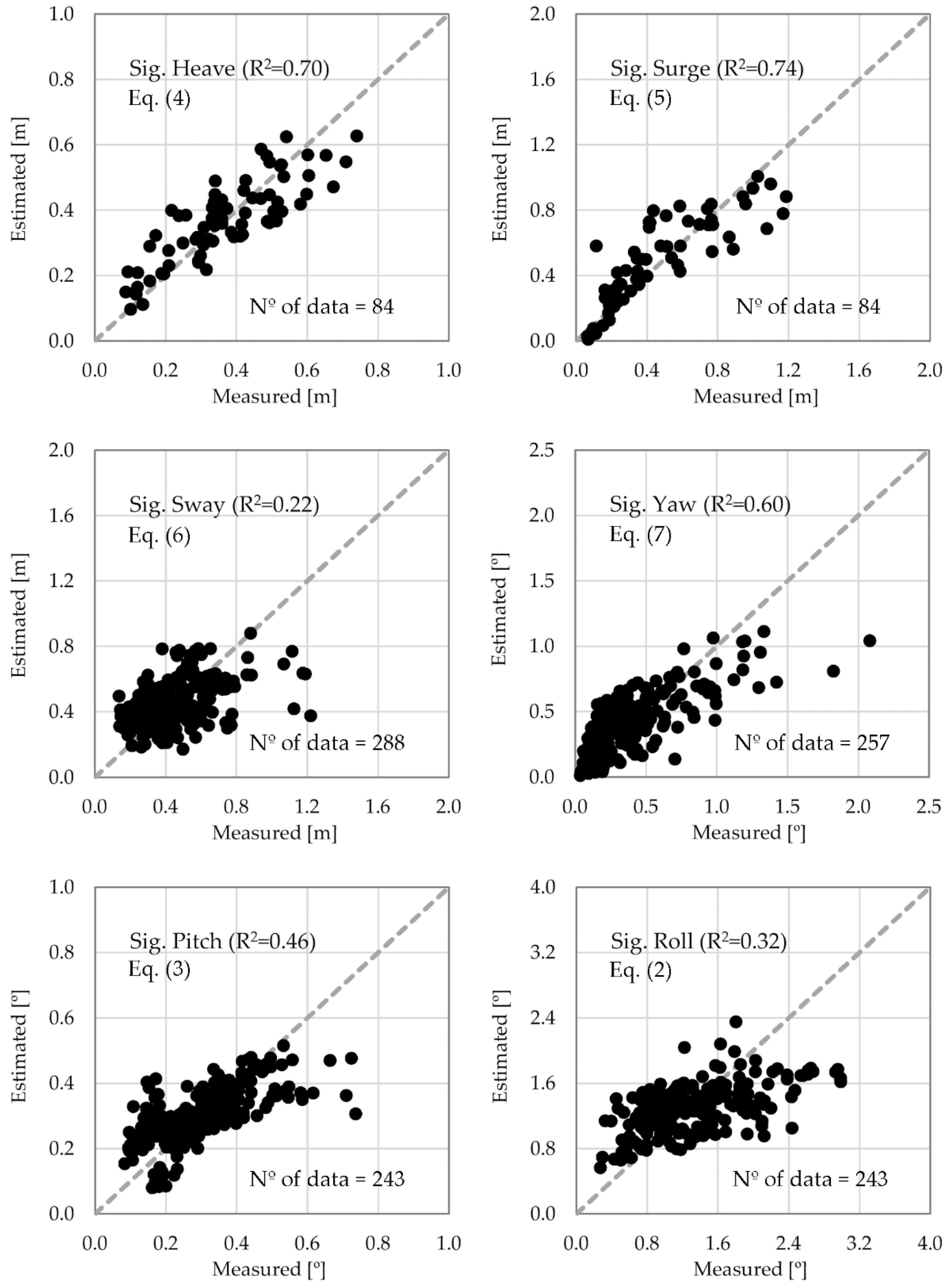
An external validation procedure was implemented in order to evaluate the predictive ability of the transfer functions compared in the previous section. For this purpose, 20% of the data obtained in the field campaigns was applied to the transfer functions and the results were compared (Figure 9).

As can be observed in Figure 9, heave, surge, yaw, and pitch estimated and measured movements conform to the bisector of the first quadrant. Sway and roll movements present a similar fit, but in a less precise way. This fact demonstrates that the proposed models achieve their objective. However, as before, the existing differences were produced by climatic characteristics, the mooring lines and the cargo configuration. 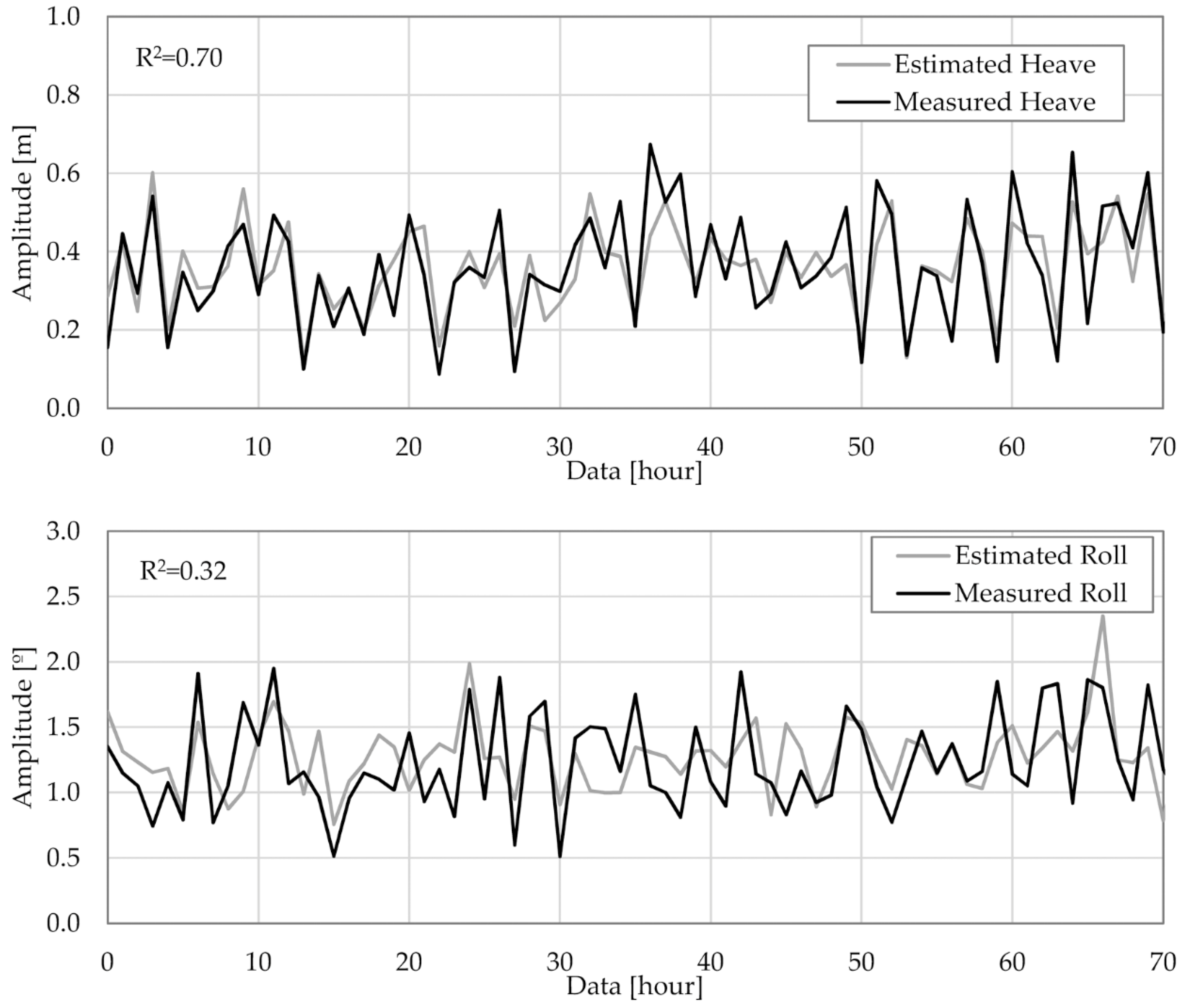Figure 10 shows the comparison between the measured heave and roll motions, and those estimated by the transfer functions from the validation data.

To quantify the accuracy of the estimations, the determination coefficient (R²) and the root mean square error (RMSE) of each movement were analyzed (

Table 11. Obtained values of the R² coefficient and the root mean square error (RMSE) in transfer functions validation.

Movement	R2	RMSE
Heave	0.70	0.08 m
Surge	0.74	0.16 m
Sway	0.22	0.18 m
Yaw	0.60	0.20°
Pitch	0.46	0.09°
Roll	0.32	0.44°

).

Comparing Table 9 and Table 11, the obtained validations reflect the same pattern as the calculated transfer functions. Similarly, both the determination coefficient (R²) and the root mean square error (RMSE) obtained were shown to be of the same order of magnitude. Therefore, it can be concluded that the accuracy of the validation is similar to that of the calculated functions. Moreover, it was also verified that the mean absolute error (MAE) had a similar value to that calculated by the models: 0.35° for the rotations, and 14 cm for the displacements (

Table 12. Mean absolute error (MAE) for each of the six degrees of freedom studied in the validation of the transfer functions.

	Mean Absolute Error
	Heave (m)	Surge (m)	Sway (m)	Yaw (°)	Pitch (°)	Roll (°)
Validation	0.07	0.12	0.14	0.14	0.07	0.35

). However, as mentioned in Section 2, these tools will be fed with weather forecast data, so their accuracy will also be conditioned by the port’s own forecasting system (Table 2).

Finally, the application of this methodology and the implementation of the obtained models in a port management system would provide reasonable predictions of the expected movements of moored vessels from weather forecast data. Comparing this information with the movement thresholds specified by the different standards would detect possible operational downtimes and risk situations in the berthing area. Therefore, this tool would help to identify operational windows for ships, facilitating decision making on port berth occupancy planning.

5. Conclusions

This paper presents an analytical methodology to relate the movements of moored vessels using the variables available in forecast data including specifically, ship dimensions and climatic conditions. This work was applied and validated for 27 moored vessels (15 Bulk carrier and 12 General cargo) at the facilities of the Outer Port of Punta Langosteira, A Coruña, Spain. The results obtained are currently incorporated in its port management system.

The results show that this methodology can be used to predict the six degrees of freedom of moored vessels. These models were obtained assuring that the variables used were independent of each other. The values of the determination coefficient (R²) and of the root mean square error (RMSE) indicate that the equations calculated allow a reasonable prediction of the movements. Even models with lower R² values (sway and roll movements) are able to estimate the main trend of the expected movements. In addition, the mean absolute error reveals that the errors are less than 14 cm for the displacements, and less than 0.36° for the rotations.

As a conclusion, it can be verified that the methodology proposed facilitates an advance towards a better understanding of the factors that influence port operations in the Outer Port of Punta Langosteira. This is the first step in order to generate warnings that assist port management and help to optimize the use of the port’s resources and facilities. Also, this methodology could be exportable to other ports providing an analysis of the influential and available forecast variables is made, as well as a record of the movements of the moored vessels.

References

1. Kumar, P.; Batra, G.; Kim, K.I. A Moored Ship Motion Analysis in Realistic Pohang New Harbor and Modified PNH. In Proceedings of the 1st International Conference on Modern Mathematical Methods and High Performance Computing in Science and Technology, M3HPCST, Ghaziabad, India, 27–29 December 2015; Springer International Publishing: Ghaziabad, India, 2016; pp. 207–214. [Google Scholar]
2. Peña, E.; Figuero, A.; Sande, J.; Guerra, A.; Perez, J.D.; Maciñeira, E. Integrated system to evaluate moored ship behavior. In Proceedings of the 36th International Conference on Offshore Mechanics and Arctic Engineering-OMAE, Trondheim, Norway, 25–30 June 2017; Volume 7A-2017. [Google Scholar]
3. PIANC. Criteria for Movements of Moored Ships in Harbours: A Practical Guide; PIANC General Secretariat: Brussels, Belgium, 1995. [Google Scholar]
4. Puertos del Estado. ROM 2.0-11. Recomendaciones para el Proyecto y Ejecución en Obras de Atraque y Amarre; Ministerio de Fomento: Madrid, Spain, 2011; ISBN 9788488975409. [Google Scholar]
5. Figuero, A.; Peña, E.; Sande, J.; Costa, F. Analysis of the movements and operational limits of moored vessels in outer and inner ports of A Coruña (Spain). In Proceedings of the 3rd International Conference on Maritime Technology and Engineering, MARTECH 2016, Lisbon, Portugal, 4–6 July 2016; Volume 1. [Google Scholar]
6. Natarajan, R.; Ganapathy, C. Model experiments on moored ships. Ocean Eng. 1997, 24, 665–676. [Google Scholar] [CrossRef]
7. Rosa-Santos, P.; Taveira-Pinto, F.; Veloso-Gomes, F. Experimental evaluation of the tension mooring effect on the response of moored ships. Coast. Eng. 2014, 85, 60–71. [Google Scholar] [CrossRef]
8. Baker, S.; Frank, G.; Cornett, A.; Williamson, D.; Kingery, D. Physical Modelling and Design Optimizations for a New Container Terminal at the Port of Moin, Costa Rica. In Ports 2016: Port Engineering Proceedings of the 14th Triennial International Conference, New Orleans, LA, USA,12–15 June 2016; Oates, D., Burkhart, E., Grob, J., Eds.; American Society of Civil Engineers (ASCE): Reston, VA, USA, 2016; pp. 560–569. [Google Scholar] [Green Version]
9. Taveira Pinto, F.; Veloso Gomes, F.; Rosa Santos, P.; Guedes Soares, C.; Fonseca, N.; Santos, J.A.; Moreira, A.P.; Costa, P.; Brógueira Dias, E. Analysis of the Behavior of Moored Tankers. In Proceedings of the 27th International Conference on Offshore Mechanics and Arctic Engineering (OMAE2008), Estoril, Portugal, 15–20 June 2008; American Society of Mechanical Engineers (ASME): New York, NY, USA, 2008; Volume 4, pp. 755–764. [Google Scholar]
10. Cornett, A. Physical modelling of moored ships for optimized design of ports and marine. In Proceedings of the 5th International Conference on the Application of Physical Modelling to Port and Coastal Protection, Varna, Bulgaria, 29 September–2 October 2014. [Google Scholar]
11. Pawar, R.; Bhar, A.; Dhavalikar, S.S. Numerical prediction of hydrodynamic forces on a moored ship due to a passing ship. Proc. Inst. Mech. Eng. Part. M J. Eng. Marit. Environ. 2019, 233, 575–585. [Google Scholar] [CrossRef]
12. Kwak, M. Numerical Simulation of Moored Ship Motion Considering Harbor Resonance. In Handbook of Coastal and Ocean Engineering: Expanded Edition; Kim, Y.C., Ed.; World Scientific Publishing Company: Singapore, 2017; Volume 2, pp. 1081–1110. [Google Scholar]
13. Pinheiro, L.; Fortes, C.J.; Santos, J.A.; Rosa-Santos, P. Numerical simulation of the motions and forces of a moored ship in Leixões harbour. In Proceedings of the 3rd International Conference on Maritime Technology and Engineering, MARTECH 2016, Lisbon, Portugal, 4–6 July 2016; Volume 1, pp. 217–226. [Google Scholar]
14. Varyani, K.S.; Vantorre, M. New generic equation for interaction effects on a moored containership due to a passing tanker. J. Ship Res. 2006, 50, 278–287. [Google Scholar]
15. Aksnes, V. A simplified interaction model for moored ships in level ice. Cold Reg. Sci. Technol. 2010, 63, 29–39. [Google Scholar] [CrossRef] [Green Version]
16. Figuero, A.; Sande, J.; Peña, E.; Alvarellos, A.; Rabuñal, J.R.; Maciñeira, E. Operational thresholds of moored ships at the oil terminal of inner port of A Coruña (Spain). Ocean Eng. 2019, 172, 599–613. [Google Scholar] [CrossRef]
17. Figuero, A.; Rodríguez, A.; Sande, J.; Peña, E.; Rabuñal, J.R. Field measurements of angular motions of a vessel at berth: Inertial device application. Control Eng. Appl. Inform. 2018, 20, 79–88. [Google Scholar]
18. Figuero, A.; Rodriguez, A.; Sande, J.; Peña, E.; Rabuñal, J.R. Dynamical study of a moored vessel using computer vision. J. Mar. Sci. Technol. 2018, 26, 240–250. [Google Scholar]
19. Gómez Lahoz, M.; Carretero Albiach, J.C. Wave forecasting at the Spanish coasts. J. Atmos. Ocean Sci. 2005, 10, 389–405. [Google Scholar] [CrossRef]
20. López, M.; Iglesias, G. Long wave effects on a vessel at berth. Appl. Ocean Res. 2014, 47, 63–72. [Google Scholar] [CrossRef]
21. Van der Molen, W.; Scott, D.; Taylor, D.; Elliott, T. Improvement of Mooring Configurations in Geraldton Harbour. J. Mar. Sci. Eng. 2016, 4, 3. [Google Scholar] [CrossRef]
22. Zelterman, D. Applied Multivariate Statistics with R; Springer International Publishing: Cham, Switzerland, 2015; ISBN 978-3-319-14093-3. [Google Scholar]
23. Carral-Couce, L.; Naya, S.; Álvarez Feal, C.; Lamas Pardo, M.; Tarrío-Saavedra, J. Estimating the traction factor and designing the deck gear for the anchor handling tug. Proc. Inst. Mech. Eng. Part. M J. Eng. Marit. Environ. 2016, 231, 600–615. [Google Scholar] [CrossRef]
24. Carral, L.; Tarrío-Saavedra, J.; Naya, S.; Bogle, J.; Sabonge, R. Effect of Inaugurating the Third Set of Locks in the Panama Canal on Vessel Size, Manoeuvring and Lockage Time. J. Navig. 2017, 70, 1205–1223. [Google Scholar] [CrossRef]
25. Carral Couce, L.; Couce, J.C.; Tarrío-Saavedra, J.; Formoso, J.A.F. Net winch design in trawlers, influence of vessel size and fishing ground. Proc. Inst. Mech. Eng. Part. M J. Eng. Marit. Environ. 2017, 233, 108–123. [Google Scholar] [CrossRef]
26. Jain, P.; Deo, M.C. Artificial Intelligence Tools to Forecast Ocean Waves in Real Time. Open Ocean Eng. J. 2008, 1, 13–20. [Google Scholar] [CrossRef] [Green Version]
27. Wang, D.; Xiong, X.L. Multivariate Linear Regression Model for Ship Traffic Flow Prediction Based on Influence Factors Analysis. Ship Ocean Eng. 2010, 3, 178–180. [Google Scholar]
28. Kutner, M.H.; Nachtsheim, C.; Neter, J.; Li, W. Applied Linear Statistical Models, 5th ed.; McGraw-Hill/Irwin: New York, NY, USA, 2005; ISBN 0072386886. [Google Scholar]
29. Burnham, K.P.; Andreson, D.R. Model. Selection and Multimodel Inference. A Practical Information-Theoretic Approach, 2nd ed.; Springer: New York, NY, USA, 2002; ISBN 978-0-387-22456-5. [Google Scholar]
Figure 1. The Outer Port of Punta Langosteira, A Coruña, Spain. The berthing line and the location of the wave buoy and the weather station used in this study are highlighted (a). Mooring arrangement of each vessel type (b).
Water 11 01841 g001
Figure 2. Left: IMU (Inertial measurement unit), Center: Photogrammetric techniques, Right: Laser distance sensor.
Water 11 01841 g002
Figure 3. Seasonal wind and wave roses (winter and summer) at the buoy position for the period 2015–2018.
Water 11 01841 g003
Figure 4. A 1 h sample of roll time series recorded on the bulk carrier vessel WESTERN BOHEME.
Water 11 01841 g004
Figure 5. Maximum, average and significant amplitudes of each motion recorded during the WESTERN BOHEME bulk carrier vessel’s stay in port and its concomitant climatic forcings.
Water 11 01841 g005
Figure 6. Cumulative frequency distribution of each of the recorded variables (Dimensionless variable range (Variable value (i)/Maximum variable value) vs. Accumulated frequency for each of the variables).
Water 11 01841 g006
Figure 7. The relative frequency corresponding to the models where the effect of each predictor on the response is significantly different from zero.
Water 11 01841 g007
Figure 8. Scatter plots of measured values versus predicted values for the multivariate linear models fitted to significant vessel movements.
Water 11 01841 g008
Figure 9. Validation of the multivariate linear models.
Water 11 01841 g009
Figure 10. Comparison between measured and estimated values of heave and roll motions.
Water 11 01841 g010