GLOF Risk Assessment Model in the Himalayas: A Case Study of a Hydropower Project in the Upper Arun River
by
 ,
,
Rana Muhammad Ali Washakh
1,2 ,
,
Ningsheng Chen
1,*,
Tao Wang
1,
Sundas Almas
3,
Sajid Rashid Ahmad
4 and
Mahfuzur Rahman
1,2,5 1
Key Laboratory of Mountain Hazards and Surface Process, Institute of Mountain Hazards and Environment, Chinese Academy of Sciences, Chengdu 610041, China
2
University of Chinese Academy of Sciences, Beijing 100049, China
3
Key Laboratory for Space Biosciences & Biotechnology, School of Life Sciences, Northwestern Polytechnical University, Xi’an 710072, China
4
College of Earth & Environmental Sciences (CEES), University of the Punjab, Punjab 54590, Pakistan
5
Department of Civil Engineering, International University of Business Agriculture and Technology, Dhaka 1230, Bangladesh
*
Author to whom correspondence should be addressed.
Water 2019, 11(9), 1839; https://doi.org/10.3390/w11091839
Submission received: 30 June 2019
/
Revised: 21 August 2019
/
Accepted: 30 August 2019
/
Published: 4 September 2019
(This article belongs to the Special Issue Impacts of Climate Change on Water Resources in Glacierized Regions)
Abstract
:A glacial lake outburst flood (GLOF) is a phenomenon that is widely known by researchers because such an event can wreak havoc on the natural environment as well as on manmade infrastructure. Therefore, a GLOF risk assessment is necessary, especially within river basins with hydropower plants, and may lead to a tremendous amount of socioeconomic loss if not done. However, due to the subjective and objective limitations of the available GLOF risk assessment methods, we have proposed a new and easily applied method with a wider application and without the need for adaptation changes in accordance with the subject area, which also allows for the repeated use of this model. In this study, we focused our efforts on the Upper Arun Hydroelectric Project (UAHEP) in the Arun River Basin, and we (1) identified 49 glacial lakes with areas greater than 0.1 km2; (2) geographically represented and analyzed these 49 glacial lakes for the period of 1990–2018; (3) analyzed the correlation between the temperature and precipitation trends and the occurrence of recorded GLOF events in the region; (4) proposed a new method based on the documented affected lengths and volumes derived from historical GLOF events to identify 4 potentially critical lakes; and (5) evaluated the discharge profiles using widely used empirical methods and further discussed the physical properties, triggering factors, and outburst probability of the critical lakes. To achieve these objectives, a series of intensive and integrated desk studies, data collections, and GLOF simulations and analyses were performed.
1. Introduction
The Himalayas are an abundant resource of water but also have a relatively poor socioeconomic status; thus, this region has been greatly utilized for hydropower projects to help alleviate power loss and poverty. Since 1935, 62 glacial lake outburst flood (GLOF) events initiated from 56 glacial lakes in the Himalayas have been recorded, of which 8 occurred in Nepal [1], and the frequency has reached 1 event every 3–10 years [2,3,4]. This area has experienced many GLOFs in the past, of which the Cirenmaco GLOF (11 July 1981) located in the Sun Koshi River Basin in China [1,4,5,6,7], the Jinco GLOF (27 August 1982) at the headwaters of the Yairuzangbo River of the Pumqu Basin in China [4], the Dig Tsho (4 August 1985) [4,8,9] and Tam Pokhari (Sabai-Tsho) GLOFs (3 September 1998) [4,10,11,12,13] in the Dudh Basin in Nepal, and the Jialongco GLOF (23 May and 29 June 2002) in the Poiqu Basin in China [14] are good examples of the destructive consequences of GLOF disasters in the Central Himalayas, resulting in the destruction of some of the major hydropower projects, further causing socioeconomic decline [4]. Therefore, before any hydroelectric plant is built in this GLOF-hazard-prone region, a GLOF risk analysis is of crucial importance [15]. As mentioned above, documented GLOF events (such as Lake Cirenmaco and Dig Tsho) in the Central Himalayas destroyed downstream hydropower stations, roads, and bridges; killed hundreds of people; and caused millions of dollars in economic losses [16]. Such GLOFs are hazardous to resident safety, properties, infrastructure (e.g., hydropower, mining, roads, and bridges), agriculture husbandry, pasturelands, forests, tourism, and socioeconomic systems in downstream regions because of their potential to cause catastrophic breaching [4,10,17].
Nepal is endowed with vast water resources, with about 6000 rivers and rivulets contributing to an annual average runoff of 225 billion m3. The total drainage of these watercourses amounts to an area of 194,171 km2, 76% of which falls within Nepal. It is noteworthy that as many as 33 of the larger rivers have drainage areas exceeding 1000 km2. The perennial nature of the rivers and the topography of the country, with steep gradients, provide excellent conditions for hydropower development, the theoretical potential of which has been estimated at 83,000 MW. In reality, however, only 1000 MW (including isolated micro and small hydropower plants)—less than 1.0% of the total potential—has been exploited so far, resulting in only 58% of the total population having access to electricity supply. The present capacity and energy generation is far less than the current electricity demand for both base and peak load and, hence, the country is forced to have load shedding during the dry season. As the electricity demand is projected to grow by 10% per year, the situation will worsen in the years to come if more sources of generation are not added to the system as soon as possible. In this context, the Nepal Electricity Authority (NEA), an undertaking of the Government of Nepal which is responsible for the generation, transmission, and distribution of electricity, has decided to initiate a detailed engineering study on hydropower projects that could be implemented at the earliest possible date. The Upper Arun Hydroelectric Project (UAHEP) is one such attractive project in the Eastern Development Region, which has very high head and firm river flow. The cabinet has also decided to implement the project through the NEA under the ownership of the Government of Nepal. In connection with this, NEA has also envisaged the development of the IkhuwaKhola Hydropower Project (IKHEP) under the umbrella of UAHEP to harness the hydropower potential of the country and to satisfy the increasing domestic power demand.
Several methods for assessing the risk of glacial lakes to outburst floods can be found in the literature [16,18,19,20,21]. These methods differentiate themselves according to the type of method structure, quantity and range of assessed characteristics, required input data, and percentage of subjectivity in assessment processes [22]. Some of them are regionally focused, and some are adjustable. The demands on input data and the rate of subjectivity of assessment procedures are generally considered as the fundamental obstructions to their repeated use. In [22], the suitability of these methods for use within the Cordillera Blanca was examined. It was shown that none of the applied methods met all of the specified criteria; therefore, a new method is desirable. Once critical lakes are identified, flood modeling and delimitation of endangered areas are the next steps in the risk management procedure [23,24].
The reasons for the presented study are as follows: First, the existing methods are not wholly suitable for use from the perspective of the assessed characteristics and the consideration of regional specificity (especially, the share and representation of various triggers of GLOFs and climate settings [22,25]). Second, the assessment procedures in the majority of these methods are at least partly subjective (based on an expert assessment without giving any thresholds when a clear instructive guide is missing); thus, different observers may reach different results even when the same input data are used. Repeated use is thus considerably limited, and this is considered the fundamental drawback of the present methods as well as a research deficit.
Due to the abovementioned reasons, the main objective of this work is to provide a comprehensive and easily repeatable methodological concept for the assessment of the risk of glacial lake hazards within the Arun River Basin, as verified using the data of glacial lakes and GLOFs recorded in this region. The impacts of glacial lake outburst floods cannot ever be completely eliminated; nevertheless, reliable assessment to identify critical glacial lakes is a necessary step in understanding the effects of flood hazards and, consequently, risk management and mitigation. Therefore, this assessment is of great importance.
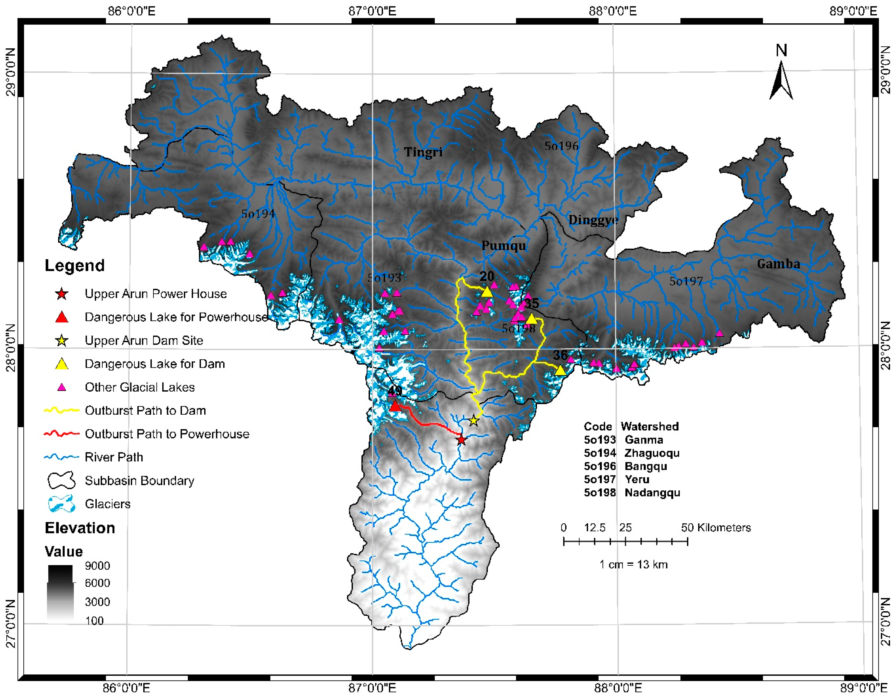
Study Area
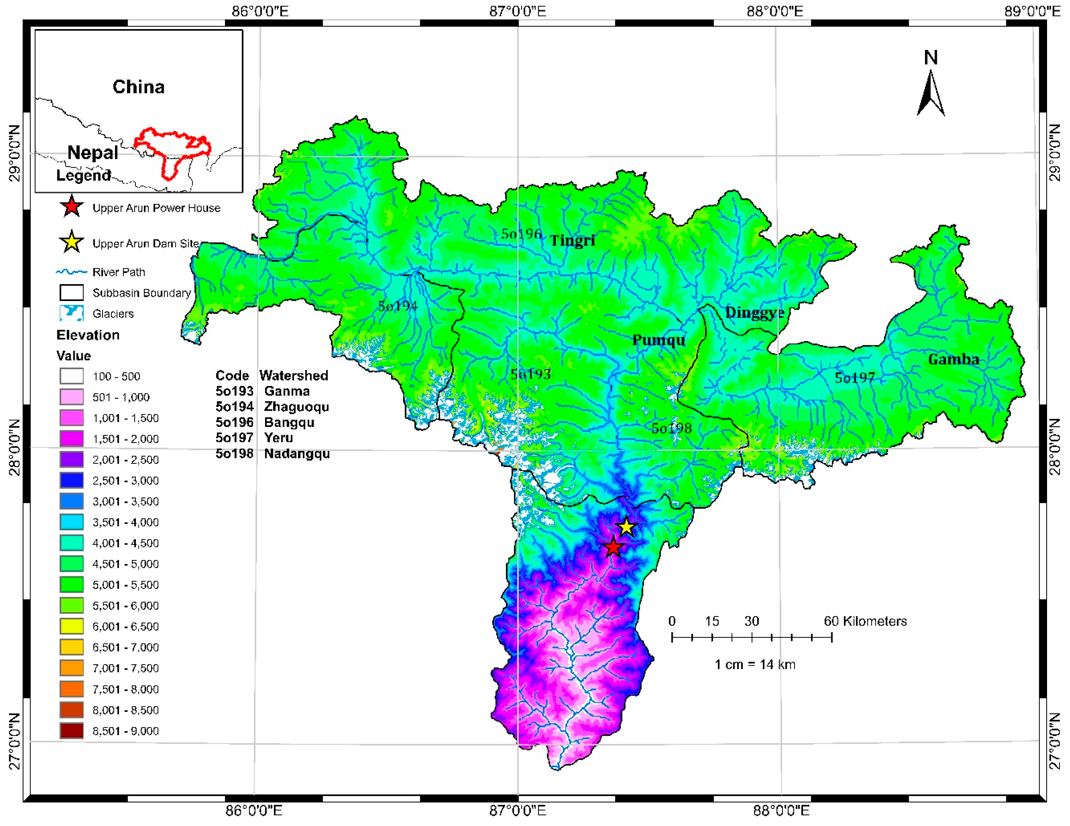
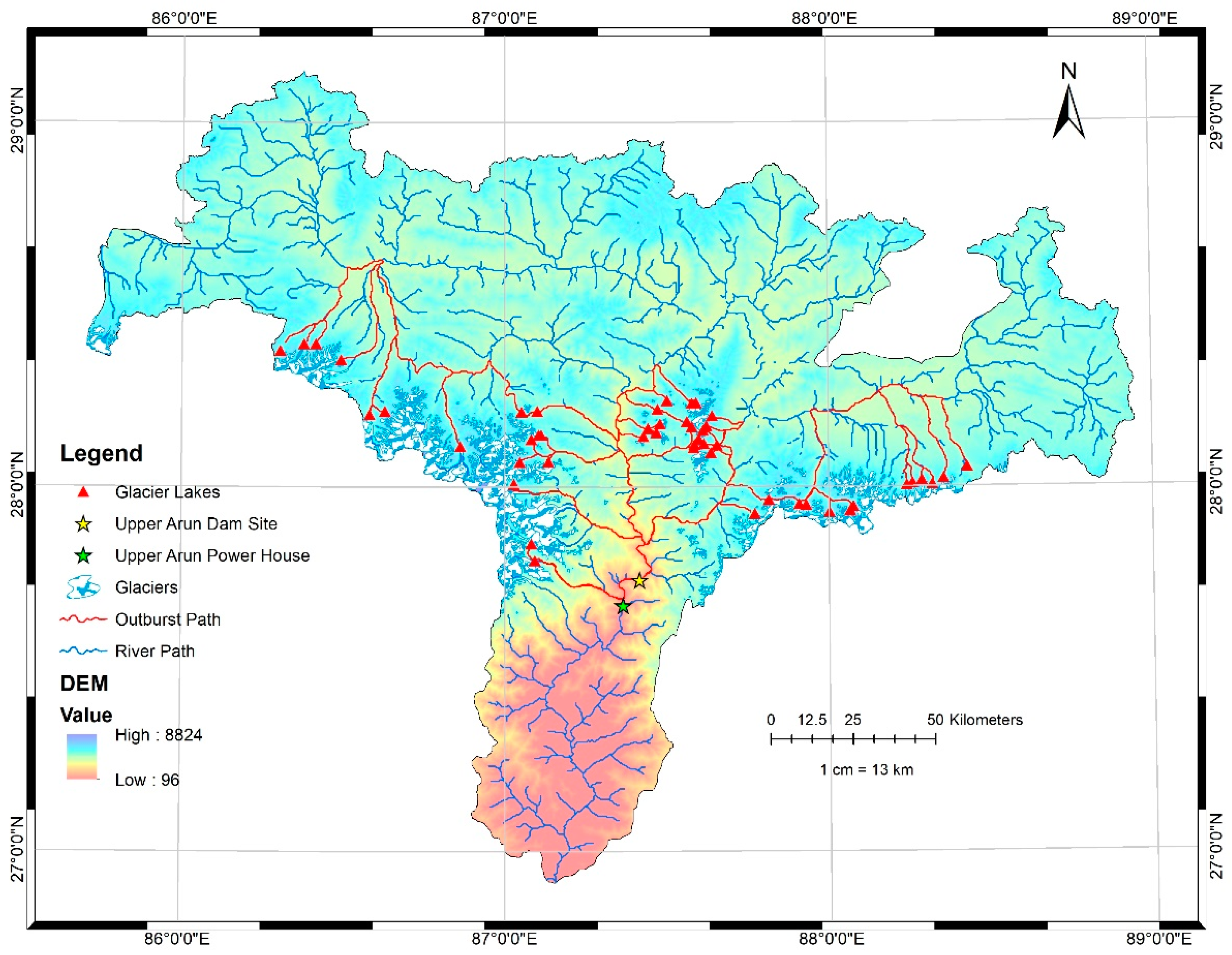
The UAHEP draws water discharged from the Arun River. It is located in the Sankhusabha District of the Koshi Zone in the Eastern Development Region of Nepal. The proposed dam site is located in a narrow gorge about 350 m upstream of the confluence with ChepuwaKhola in Chepuwa Village. The powerhouse lies in Hatiya Village, near the confluence of the Arun River with LeksuwaKhola. The project area is situated within longitudes 87°20’00” to 87°30’00”E and latitudes 27°38’24” to 27°48’09”N, as presented in Figure 1. The project area is located approximately 700 km east of Kathmandu and approximately 300 km north of Biratnagar. Fifty-two hydropower project sites have been identified within the Koshi Basin alone, and the proposed UAHEP is among the highest priorities of projects fed by mountain glaciers, which is why a GLOF risk assessment is one of the most important parts of this project.
In 1985, the project site for UAHEP was recognized during the Master Plan Study of the Koshi River (Water Resources Development, JICA). In the summer of 1986, NEA conducted a reconnaissance study. In 1991, the Joint Venture of Morrison Knudsen Corporation, Lahmeyer International, Tokyo Electric Power Services Co., and NEPECON carried out a feasibility study of this project on behalf of NEA. NEA has given priority to the development of this project to augment the energy generation capability of the integrated Nepal Power System due to its relatively low cost of generation and availability of abundant firm energy. The feasibility study carried out in 1991 chose an installed capacity of 335 MW for the peaking run-of-river-type UAHEP. The design discharge of the project was 78.8 m3/sec, and it was expected to generate firm energy of 2050 GWh per year. In 2008, NEA obtained a license from the Government of Nepal to develop the UAHEP. The updated estimated cost was US$446 million (335 MW/2050 GWh).
2. Materials and Methods
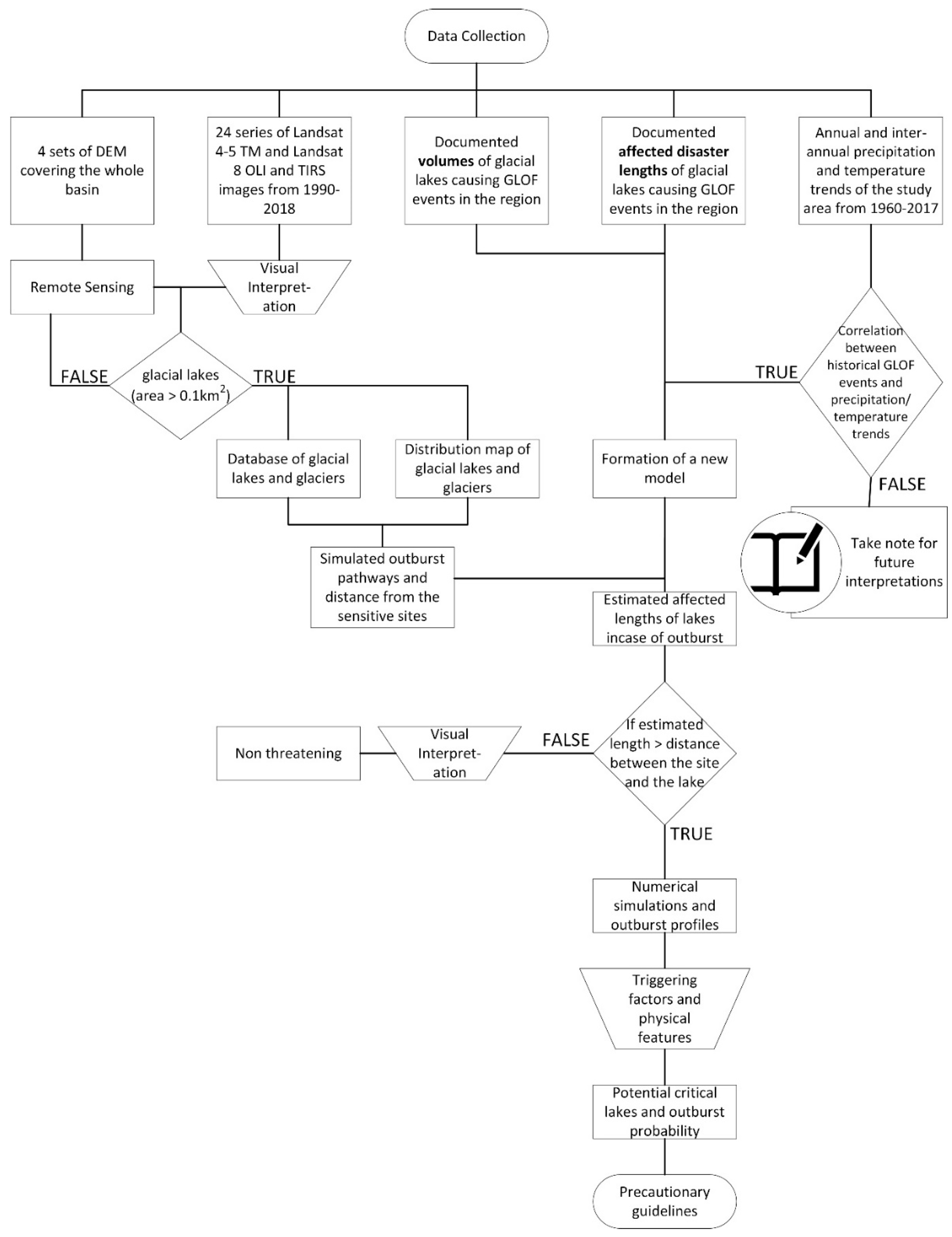
A detailed systematic methodological pathway is presented in Figure 2. This mainly included collected data in the form of satellite images, details of the historical GLOF events in the form of recorded volumes of the lakes and their corresponding affected lengths in the event of an outburst, and climatic data of the region, which were then analyzed through geographical information systems and statistical and analytical techniques. This methodology resulted in a new GLOF risk assessment model which was then applied to identify potentially critical glacial lakes.
2.1. Data Collection
The data collection included four sets of digital elevation models (DEMs) covering the whole basin and satellite images, namely, 24 series of Landsat 4–5 Thematic Mapper (TM) [26], Landsat 8 Operational Land Imager (OLI), and Thermal Infrared Sensor (TIRS) from 1990 to 2018 US Geological Survey images, with four images for each year mosaicked to cover the whole basin for the years 1990, 1995, 2000, 2005, 2011, and 2018, resulting in a total of 24 satellite images. Data related to daily, monthly, and annual average temperatures, as well as precipitation for the years 1960–2017, were collected from the China Meteorological Data Service Center (CMDC). We also formed a database of documented volumes and affected disaster lengths of historical GLOF events in the region.
2.2. Remote Sensing
An advanced automated adaptive lake mapping method was adopted to interpret remote sensing images based on relevant maps to discover the distribution and annual and interannual changes of glaciers and glacial lakes in the basin. Geometric parameters of glacial lakes as well as their physical properties and river course characteristics were obtained through field investigation. These data were used to establish glacial lake databases and plot the distribution maps of glaciers and glacial lakes in the research area.
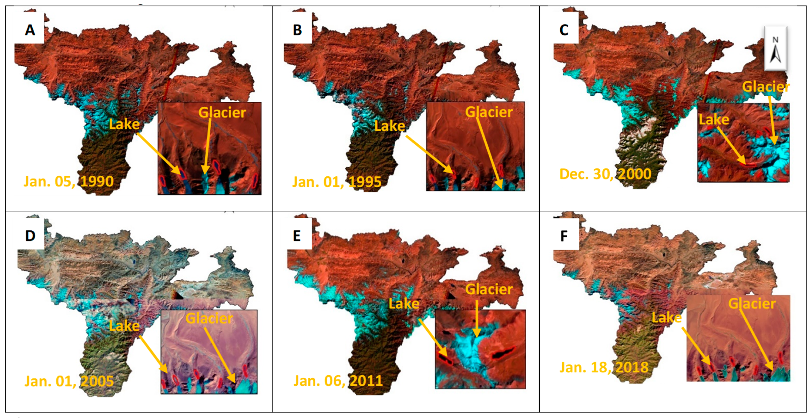
The lakes at risk are situated in remote and inaccessible areas. Remote sensing provides a feasible method to monitor glacial lakes [17]. An advanced adaptive lake mapping method was used to interpret remote sensing images (e.g., TM, Landsat 8, and other high-resolution images) based on relevant maps so as to determine the distribution, morphological characteristics, and annual and interannual changes of glaciers in the basin. Geometric parameters of glacial lakes, the physical properties of moraines, the depth of the lake, parameters of feeding glaciers, and river course characteristics were determined through field investigation and remote sensing analysis, as demonstrated in Figure 3.
In total, we acquired 24 series of Landsat 8 OLI/TIRS images with no or less than 20% cloud cover for the periods of November–January in the years 1990, 1995, 2000, 2005, 2011, and 2017. The images used in this study were level 1 Geospatial Tagged Image File Format (GeoTIFF) data products, which were preliminarily calibrated. DEM data with a resolution of 90 m from the Shuttle Radar Topography Mission (SRTM) were used to obtain topographic information.
In this study, panchromatic images (band 8) from Landsat 8 OLI were registered with digital topographic maps using Earth Resource Data Analysis System (ERDAS) Imagine software. The registration accuracy was within 15 m (one pixel) in most areas. Furthermore, the images of other bands were resized to 15 m and were registered using the reference information from the panchromatic band.
The manual identification of individual glaciers was coupled and supplemented with the Global Land Ice Measurements from Space (GLIMS) database [10,27,28], so that the results could be merged and double-checked [28] to create an updated database. Since an individual dataset from GLIMS, ICIMOD, or CAS was not sufficient, we applied a combination of the three in addition to visual interpretation. A manual interpretation method was used to outline the glaciers and glacial lakes based on false color composite (FCC) images (6, 5, and 3 bands). DEM data were used to determine the dividing line of conjunct glaciers. The accuracy of manual interpretation has been demonstrated as optimal for identifying glaciers and glacial lakes because it allows for the consideration of both spectral characteristics and information regarding texture, patterns, shapes, and shadows. Finally, the spatial attributes of glaciers and glacial lakes were calculated using the topological analysis function of ArcInfo software based on the DEM data, and the volumes of glacial lakes were calculated based on their areas.
2.3. Formation of the Model
The main objective of this research is to determine the potential critical glacial lakes that could endanger the Hydroelectric Project. According to the results of remote sensing, there are 49 lakes with areas larger than 0.1 km2. In this study, we selected the affected length to determine the potential critical glacial lakes. Firstly, we collected the affected lengths of historical GLOFs that had occurred in the Himalayan region. Secondly, an empirical equation was presented based on the collected data. Thirdly, the presented equation was used to predict the affected lengths of the 49 lakes. The lakes were determined as critical glacial lakes when the predicted affected length was longer than the distance between the lake and the dam (powerhouse) site.
3. Results
3.1. The New Model
Data including lake volumes and affected lengths from 11 historical GLOFs in the Himalayan region were collected. The detailed data are listed in Table 1.
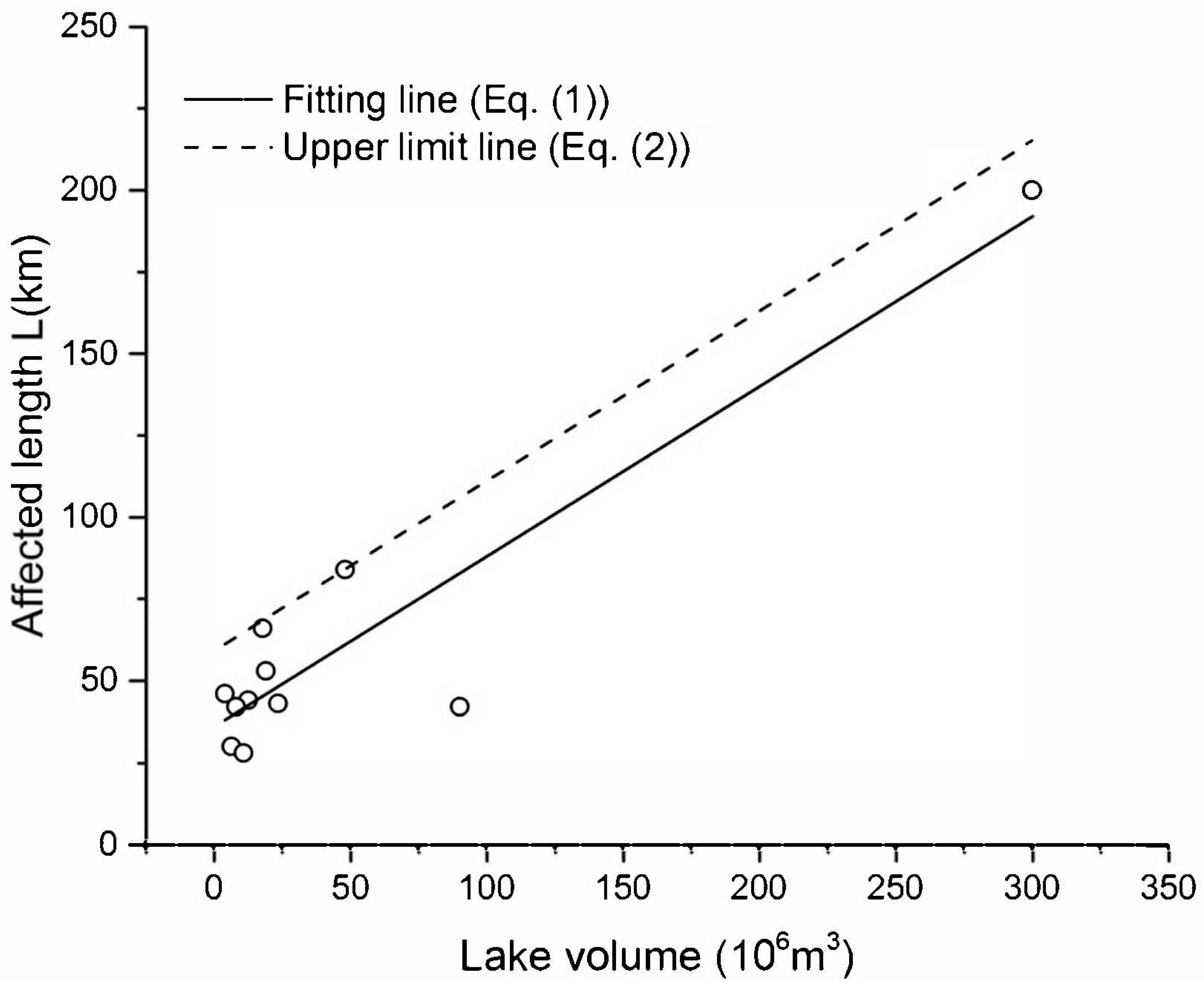
As shown in Figure 4, the affected length increases with the increase in lake volume. The fitting equation can be described as
where L is the affected length in km, and V is the lake volume in 106 m3.
L = 0.52V + 36.13
Additionally, the upper limit line can be described as
L = 0.52V + 59.21
3.2. Determination of the Critical Lakes
After the formulation of the model, glacial lake databases were established, and the distributions of glaciers and glacial lakes in the research area were mapped. Furthermore, by carefully examining the elevations and flow paths, the expected outburst paths to the dam site were simulated (Appendix A, Figure A2) and individual distances between glacial lakes and the dam site were calculated in kilometers, as illustrated in Table 2. Table 2 summarizes the glacier inventories in the Arun River Basin for the years 1990–2017, including glacial lake locations with respect to longitudes and latitudes in decimal degrees followed by glacial lake areas in square kilometers.
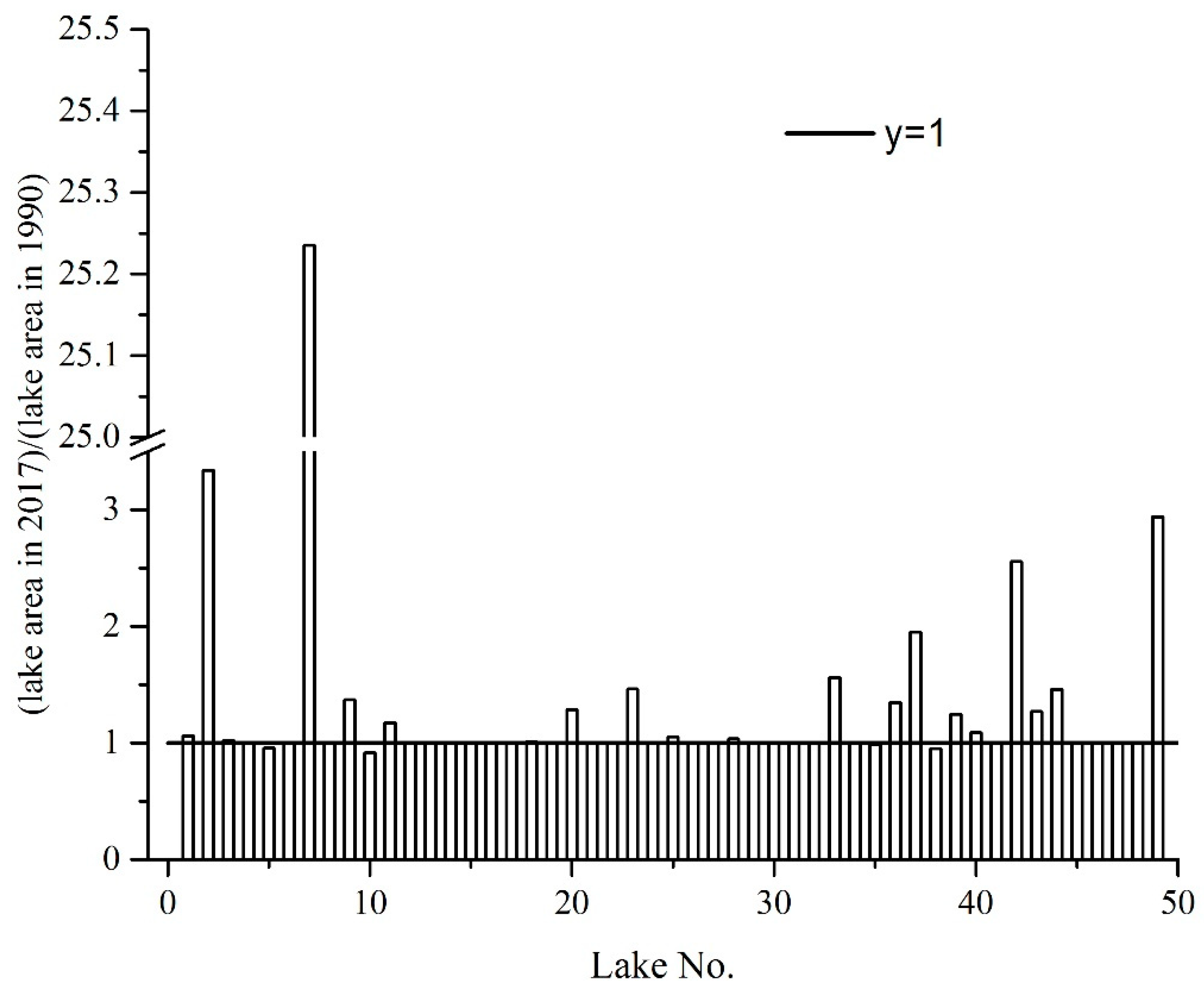
The sum of the lake area for the 49 lakes increased from 23.65 to 28.76 km2. The ratio of the sum of the lake area in 2017 was 1.22 times that in 1990 because of the gradual increase in feeding from the mother glaciers and increased precipitation in the region.
In this study, the ratio of a lake area in 2017 to that in 1990 is defined as R. As shown in Appendix A, Figure A1, there are 20 lakes with R-values larger than 1. This indicates that the lake areas of the 20 lakes increased from 1990 to 2017. The maximum R is 25.23. There are 25 lakes with R-values remaining unchanged. There are four lakes with R-values less than 1. This indicates that the lake areas of these four lakes decreased from 1990 to 2017. The minimum R is 0.92.
Equation (2) was adopted to predict the affected length. The detailed data of lake volume, affected length (Lc), and distance between the lake and the Upper Arun dam site (Ld) are listed in Table 2. As shown in Table 2, the ratios of Lc to Ld of nos. 13, 20, 33, 35, 36, and 42 are larger than 1.0; this indicates that the possible GLOFs of these six lakes may endanger the dam.
The detailed data of lake volume, affected length (Lc), and distance between the lake and the Upper Arun powerhouse (Lp) are listed in Table 2. As shown in Table 2, the ratios of Lc to Lp of nos. 11, 35, 36, and 49 are larger than 1.0; this indicates that the possible GLOFs of these four lakes may endanger the Upper Arun powerhouse.
As shown in Table 2, six glacial lakes were identified as potentially critical glacial lakes (nos. 13, 20, 33, 35, 36, and 42) for the Upper Arun dam. We selected three potential critical glacial lakes (nos. 20, 35, and 36). For these three lakes, the values of Lc/Ld are larger than 1.15. These three lakes are the most critical for the Upper Arun dam. The detailed distribution of these three potential critical glacial lakes is shown in Figure 5.
As shown in Table 2, four glacial lakes were identified as potentially critical glacial lakes (nos. 11, 35, 36, and 49) for the Upper Arun powerhouse. We selected glacial lake no. 49 as the most critical lake because the value of Lc/Lp is much larger than those of the other three glacial lakes (nos. 11, 35, and 36) (Table 2).
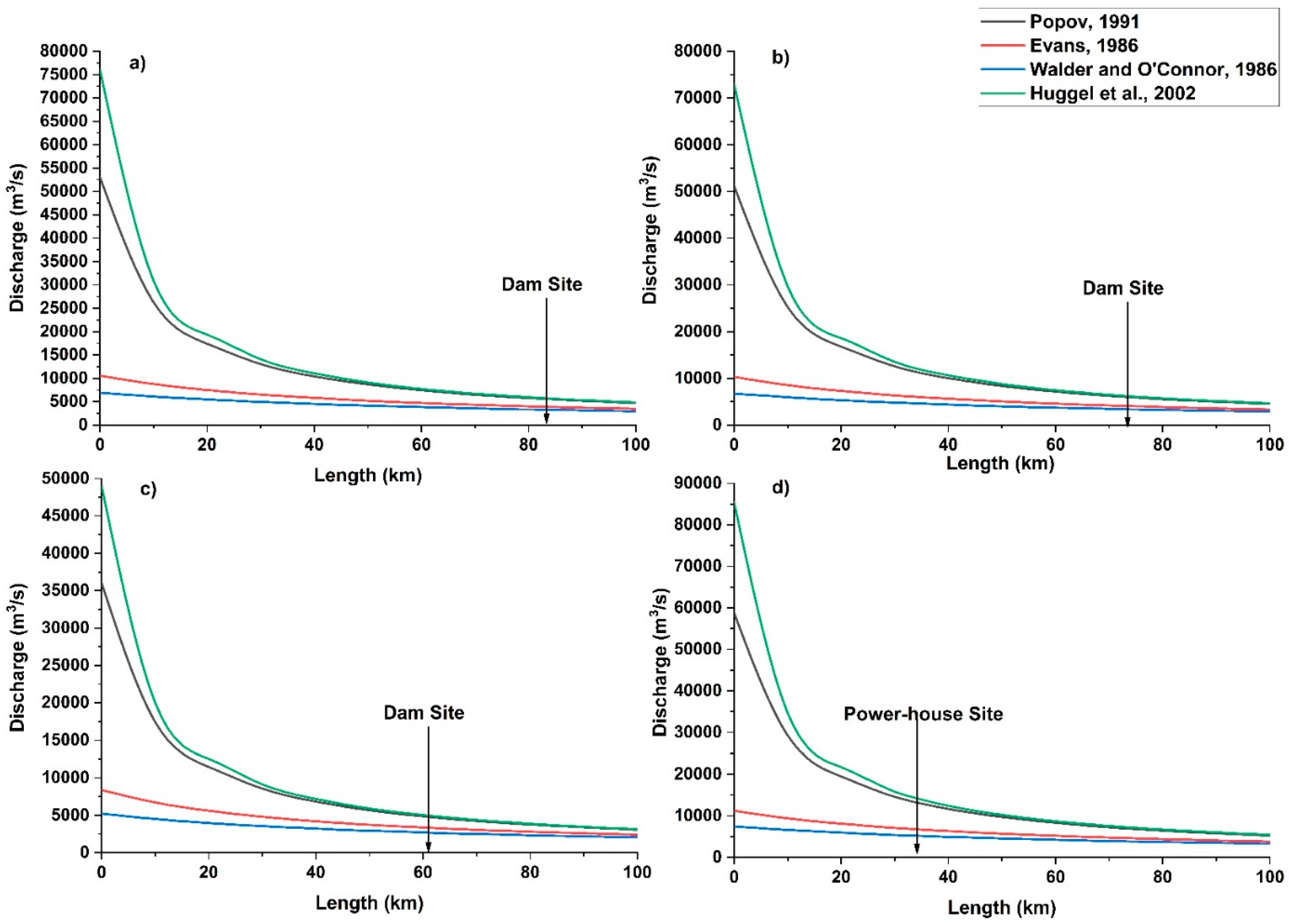
3.3. Discharge Profiles and Outburst Probability of the Critical Lakes
The peak discharge at a cross section was calculated using an empirical formula [38]:
where Vw is the volume of water (m3); Qm is the peak discharge at the dam site (m3/s); Qxm is the peak discharge at a cross section (m3/s); L is the distance from the dam (m), and vwK is an empirical coefficient equal to 3.13 for rivers on plains, 7.15 for mountain rivers, and 4.76 for rivers flowing through terrain with intermediate relief.
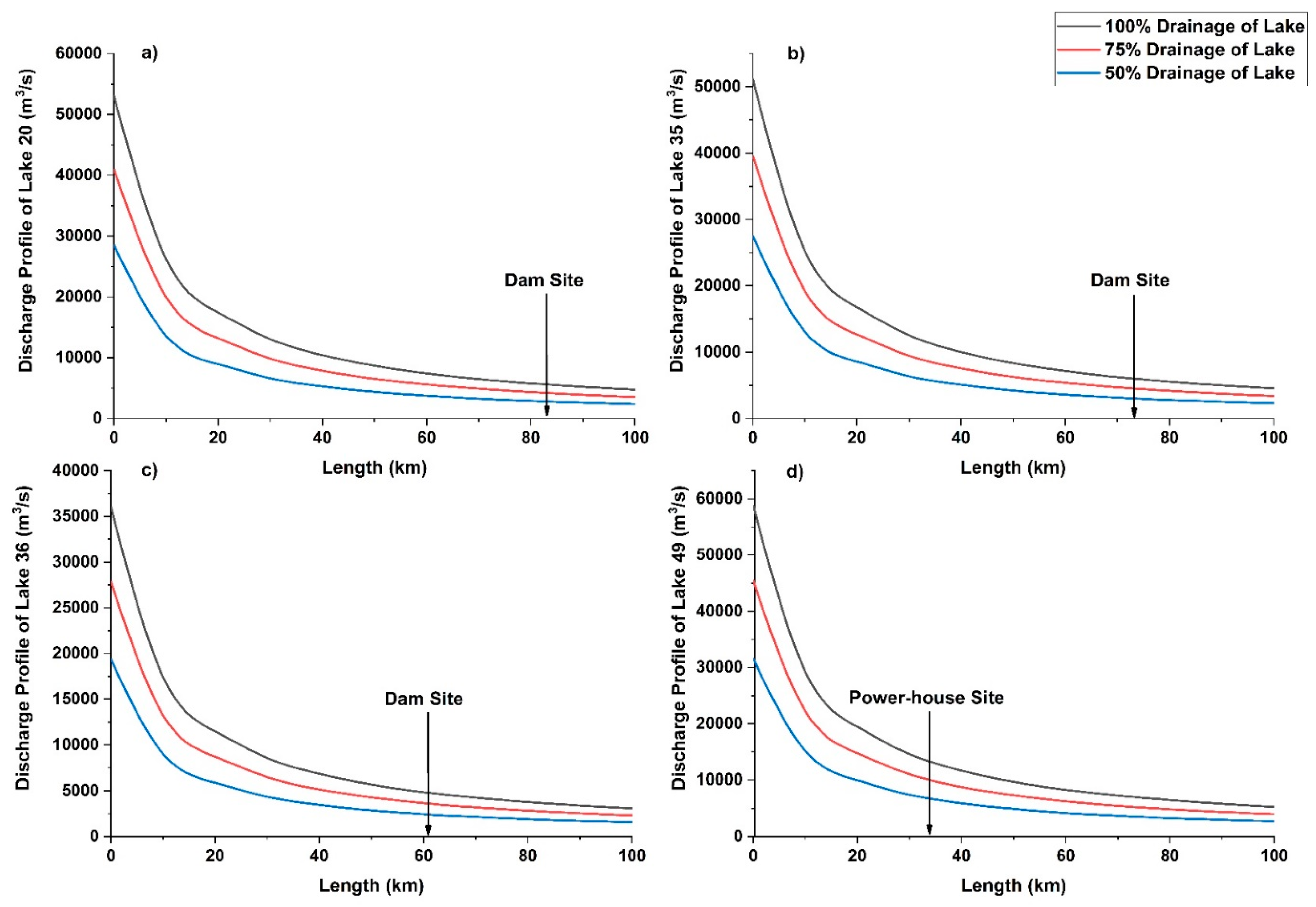
GLOFs caused by the collapse and erosion of moraine dams seldom result in the drainage of 100% of the total lake volume. GLOFs caused by avalanche push (seiche) waves also do not normally mobilize 100% of the lake volume. However, it is difficult to predict how much volume will be mobilized; therefore, it is necessary to identify and discuss different scenarios, which include 100%, 75%, and 50% drainage of the lake volume to minimize the maximum and minimum potential risks (Figure 7, Table 4).
As shown in Appendix A, Figure A4, among the identified potential glacial lakes, lake no. 35 seems the most stable considering the change in the area over the past 28 years, while lake no. 49 seems to be the most unstable in this regard. Physical features of the critical dams are recorded in Table 4 above and are visually interpreted in Appendix A, Figure A3.
Furthermore, previous studies have shown that moraine-dammed lakes have higher probabilities of outburst than those of landslide-dammed or erosion lakes [24]. Lake no. 39 (moraine lake, glacier at the end) and no. 49 (moraine lake, glacier tongue deep into the lake) are identified as being moraine dammed and possessing unstable geometry due to the rapid change in their glacial lake area over recent decades. Along with the potential impacts of ice avalanches and rock fall because they are closer to the mother glacier, this makes their outburst probabilities higher compared with the other two lakes. Additionally, the volume of lake no. 49 is the largest among the four critical lakes, and the higher the volume of a moraine-dammed lake, the higher the possibility of outburst [24]. By contrast, lake no. 20 is a landslide-blocking lake, and glacial lake no. 35 is a glacial erosion lake, both of which are not easy to break; thus, it can be concluded that lake nos. 36 and 49 should be considered as having high outburst probabilities (Table 4).
4. Discussion
4.1. Climatic Correlation with GLOFs
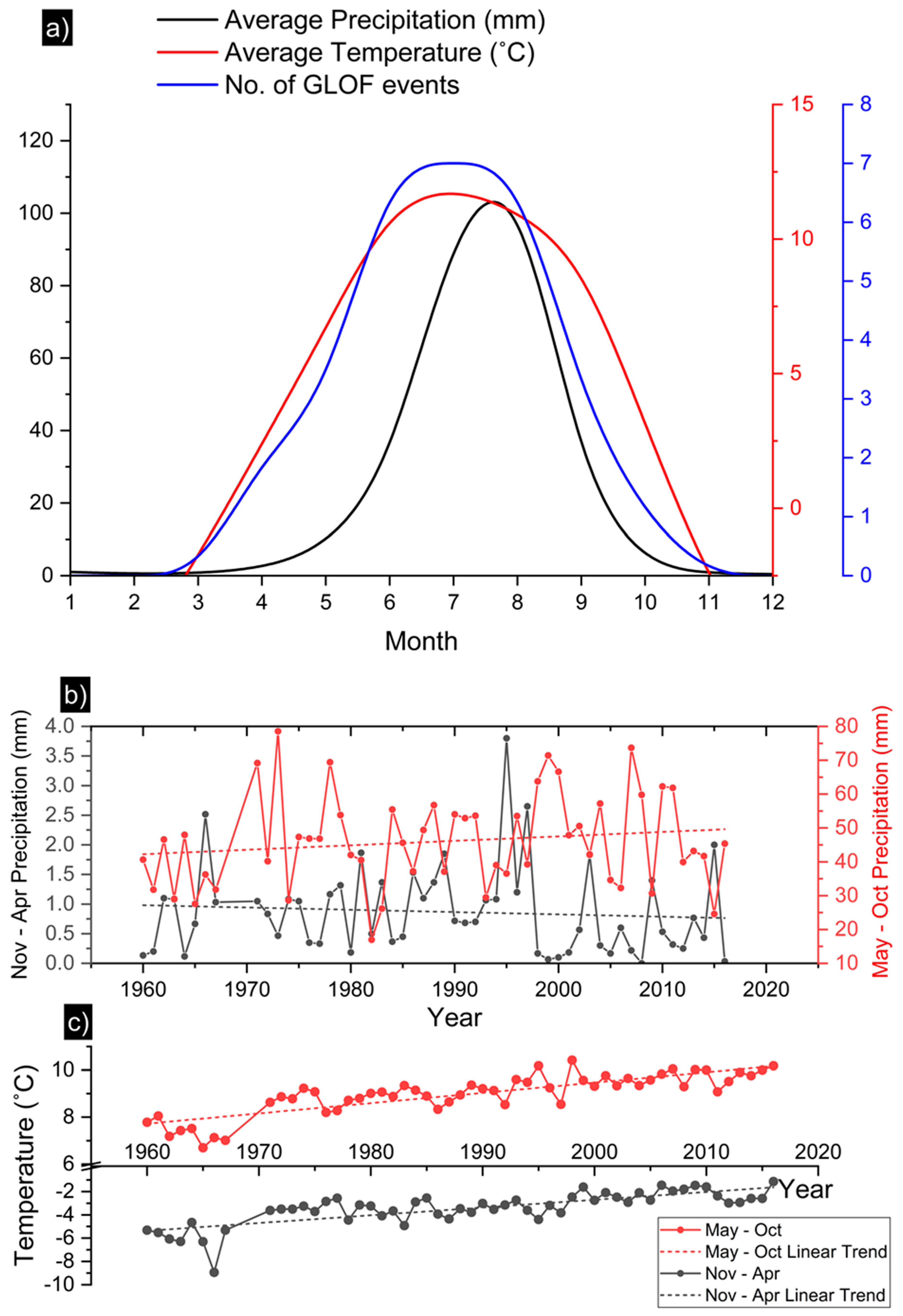
Data regarding the monthly annual average rainfall for the period of 1960–2017 are represented in Figure 8b, which clearly suggests that the monsoon season starts in May and ends in October, reaching the peak monthly average value of over 100 mm in August. Moreover, the rest of the year is dry. There is a rise in monthly annual average temperature from April to July, reaching a peak of about 12 °C in June, and then a steady decrease until November. Following a steep fall from October until January, the lowest average value of −7.5 °C is in January.
The seasonal distribution of the precipitation in the project area within Nepal is dominated by a rainy season from May through September, when the monsoons bring 90% of the annual precipitation, and a dry season from November through April. Due to the high elevation and low temperatures in most parts of the Arun River Basin, a certain portion of the precipitation is in the form of snow. No snowfall records are available for the Nepalese portion. Based on records available for the Tibetan region, annual snowfall generally increases with the increment in elevation. At an elevation of 4000 m, about 15%–22% of the annual precipitation falls as snow, and 30%–40% at 4500 m elevation. Snowfall is generally recorded from November through March.
There seems to be an increasing trend in the monsoon season (i.e., from May until October), with the peak seasonal annual rainfall of about 80 mm in the years 1970–1975. However, the opposite can be seen in the dry season (i.e., from November to April), with a minimum of no rainfall and a maximum of just below 4 mm.
In Figure 8c, an overall temperature increase is observed with some minor variations over the past 47 years, with the lowest temperature of −9 °C in the seasonal annual average from November to April, and a maximum in the range of 8–10 °C. The trend line also suggests an increase in the future. In general, Dingri County exhibits a cold climate, though it is expected to take a similar course as the regional temperature rises.
As shown in Figure 8a, there seems to be an apparent relationship between the increases in temperature and precipitation and the resulting increase in the frequency of glacial lake outbursts. Statistics based on the 27 well-recorded GLOF events show that all of them occurred between May and October (Figure 8a), with the majority (18) occurring between June and August. Summarized as an annual cycle, a GLOF can start as early as the beginning of May, for example, the Jialongco event on 23 May 2002, while the latest GLOF may happen in early October, such as the Luggye Tsho event on 7 October 1994. These statistics imply that GLOFs rarely occur during the frozen period from November to March. Rapid warming and precipitation during the ablation season cause ice avalanches and generate massive glacier melt water [5,12], both of which are prone to triggering a GLOF as a result of dam failure. It can be said that in future years, the scale of GLOF events may increase as the annual temperature and precipitation also increase; however, the influence of climate change on the frequency of GLOFs is very complex. A recent study [39] showed that the average annual frequency of GLOFs had no credible posterior trend, despite reported increases in glacial lake areas in most of the Kush–Karakoram–Himalaya–Nyainqentanglha area. Therefore, the relationship between climatic features and the frequency of GLOF events is still unclear.
4.2. Justification for the Assumed Depth of the Lakes
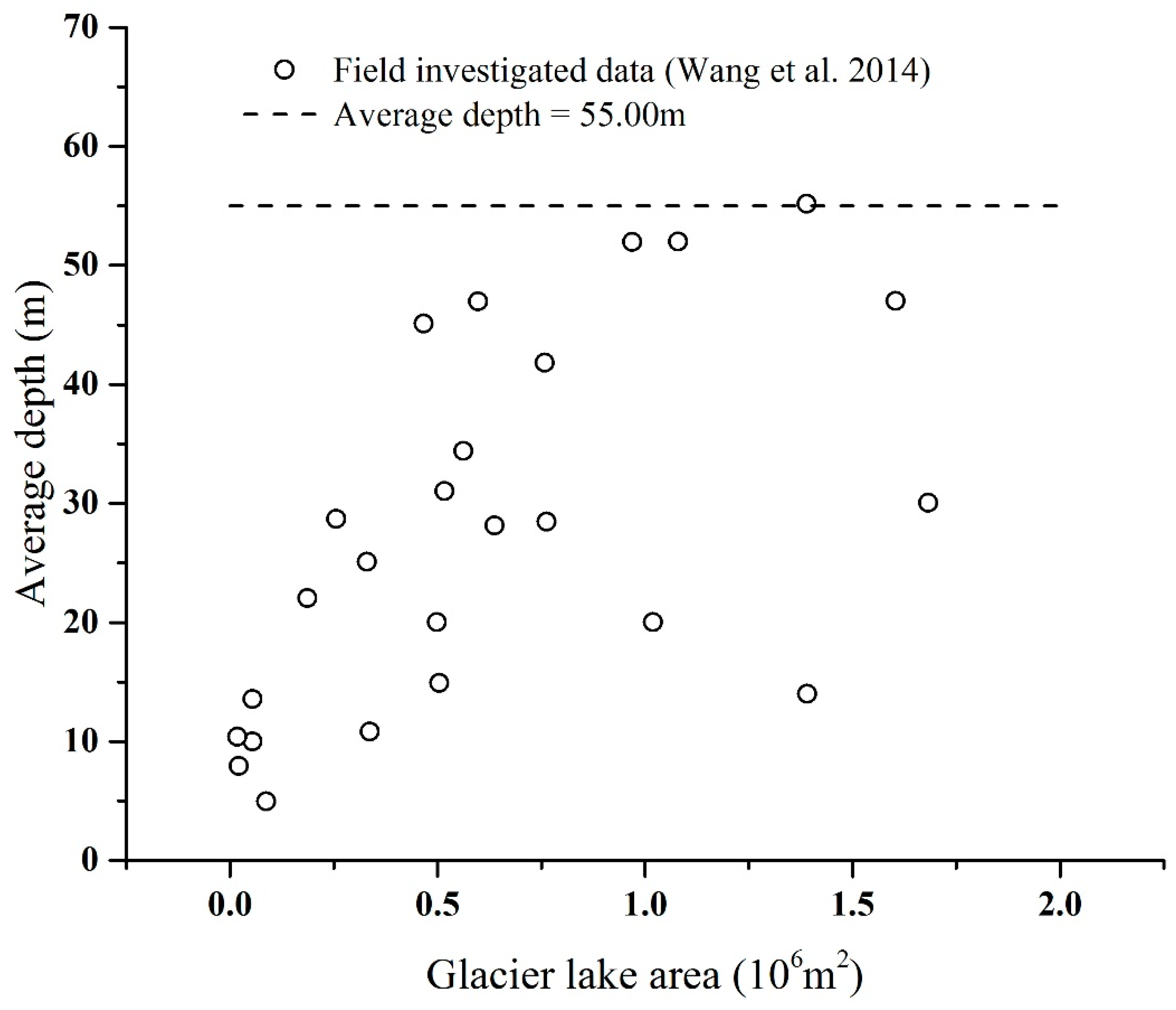
The distances between glacial lakes and the dam (powerhouse) site were obtained from DEMs. It is difficult to obtain the average depth of glacial lakes. A previous study showed that the maximum depth of glacial lakes in the Himalayan region was 55 m. In this study, it was assumed that the depth of the 49 lakes is 55 m [40]. Figure 9 shows the relation between the average depth of lakes and the moraine lake area in the Himalayas. The average depth of lakes and the moraine lake area were obtained through field investigation. However, it is appropriate for us to assume that the average depth is 55 m for lakes with areas larger than 0.80 km2. We conducted numerical simulations for four lakes (nos. 20, 35, 36, and 49). The areas of the four lakes each exceed 0.80 km2.
4.3. Analysis, Limitations, and Recommendations in Relation to the Model
The model is based on the influenced lengths of 11 historical GLOF events, and the reason for choosing the upper limit line (Equation (2)) is that it covers more data than the best-fit line. The findings of our study identify lake nos. 20, 35, 36, and 49 as the most critical due to their location, volume, physical features, and distance from both the Upper Arun dam and powerhouse. In other words, the values of Lc/Ld or Lc/Lp are large enough to pose serious risks as compared to all the other glacial lakes. Although lake no. 11 is in close proximity to lake no. 49, its lesser volume and more stable dam geometry (and thus, lower potential discharge) make it nonthreatening in the case of an outburst. This model is not only limited to the Himalayas but can also be applied to other mountainous regions. The results of this study investigating and analyzing the influence of GLOFs on the Upper Arun Hydroelectric Project and IkhuwaKhola Hydropower Project were peer-reviewed and accepted by a joint venture (CSPDR-SINOTECH JV) led by the Changjiang Institute of Survey, Planning, Design, and Research (CSPDR) with the NEA for the project entitled “Detailed Engineering Design and Preparation of Bidding Documents for Construction of Upper Arun Hydroelectric Project and IkhuwaKhola Hydropower Project”.
The number of historical GLOF events used to devise the model is limited, while a larger dataset could strengthen the numerical relationship between the volume and the affected length of a GLOF. The reason for the restricted set of data used to derivate the model is that the influenced lengths of most past GLOFs were not recorded. Moreover, a quasi-process such as an earthquake can trigger a GLOF hazard, regardless of the volume and distance of the glacial lake from the site of the assessed project. Another factor that needs to be addressed is the fact that a chain outburst of glacial lakes can happen, but prediction of such an event requires further study.
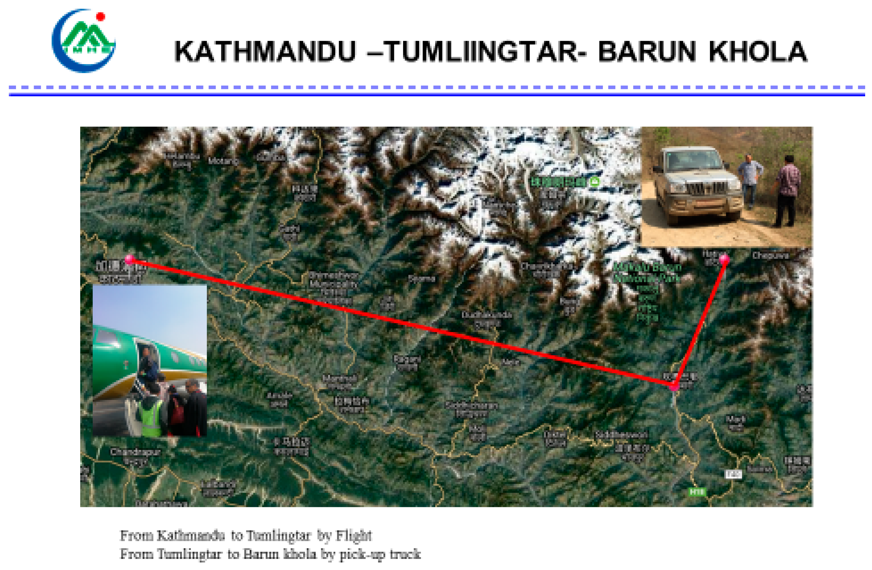
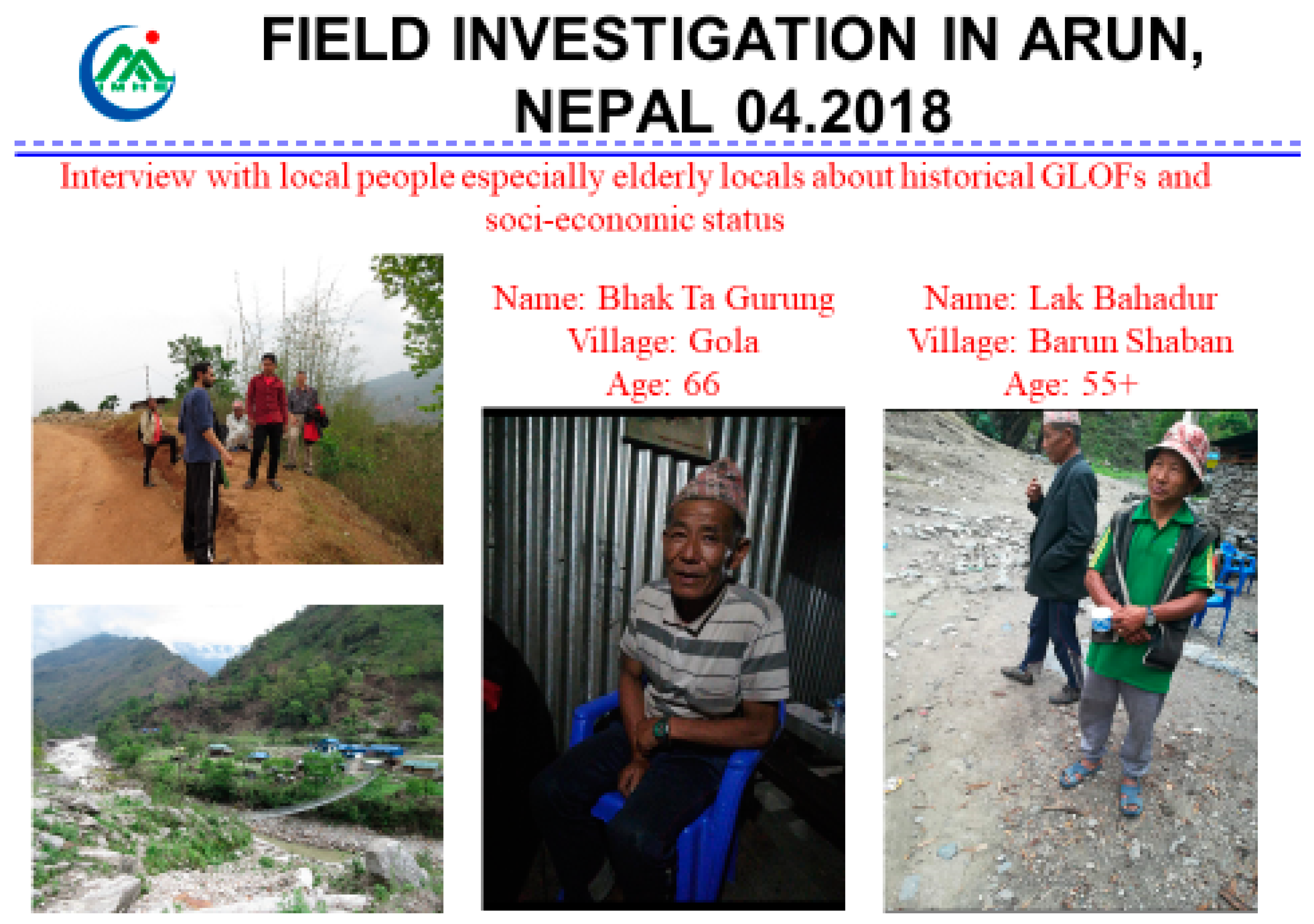
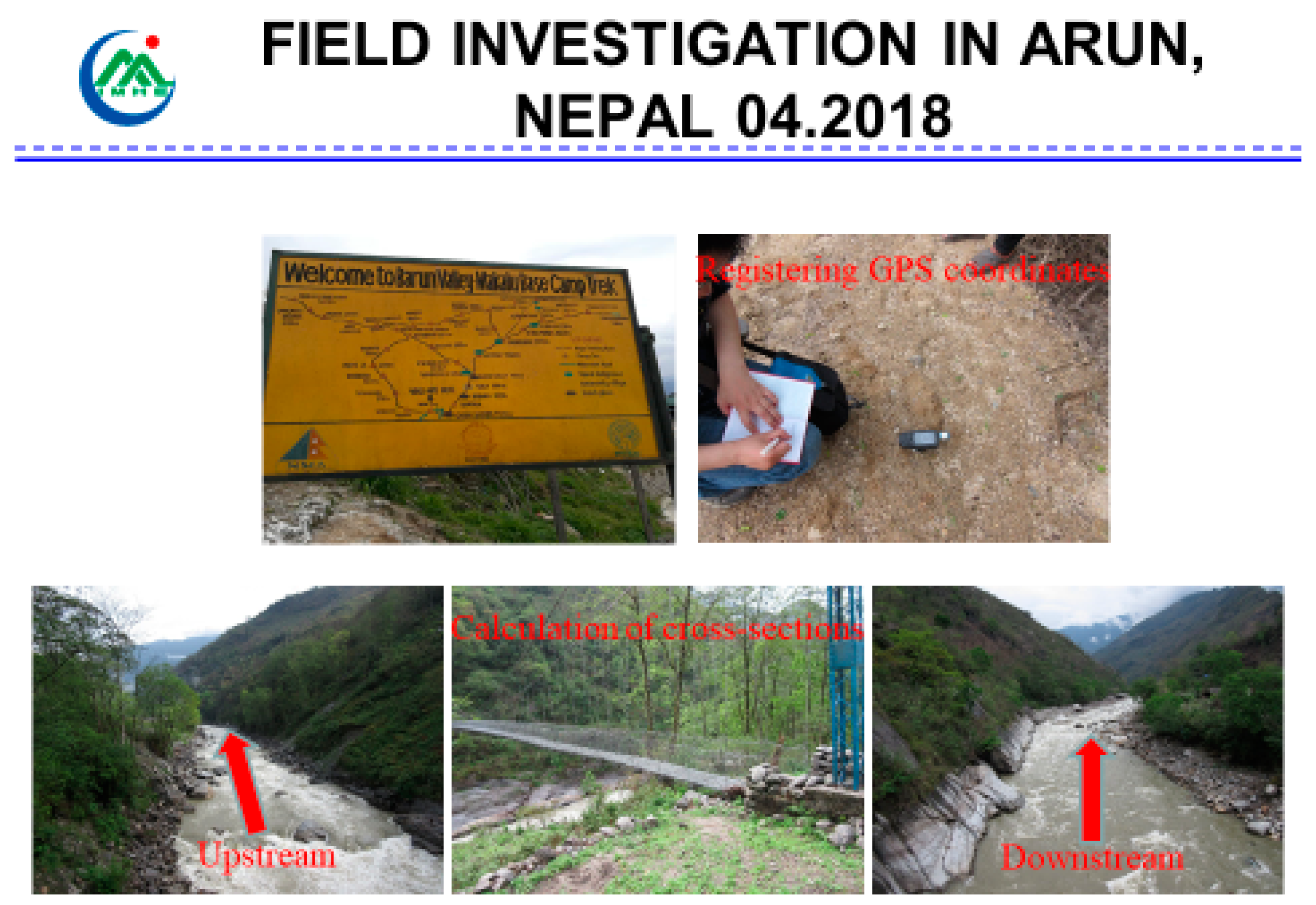
The field visit by our research team in April 2018 (Appendix A, Figure A5, Figure A6, Figure A7 and Figure A8) concluded that the topography and characteristics of the river channel are fairly consistent over the studied site [41]. Thus, these two factors were eliminated in the proposed model to minimize the uncertainties in the results. Although it would be very challenging, in future studies, characteristics of the river channel and an integrated model may be proposed incorporating more factors. It may also be possible to explore the possible destruction-triggering mechanism for each glacial lake in addition to the four critical lakes analyzed in Section 3.3. However, it would be very difficult to discuss the failure of a glacial lake dam under different triggering factors. It is important to address the factors that affect GLOF fluctuation, such as the outburst dynamic process and the scale. Nevertheless, to accomplish this task, the most basic step is to collect samples—which is not easy, as the terrain and environment at the glacial lakes’ sites make it impossible to physically travel there—and to test the particle size and mechanical parameters of the samples.
5. Conclusions
Extensive remote sensing identified 49 lakes with areas larger than 0.1 km2, namely, lake nos. 1–10 and 12–48, which are located upstream of the dam site, and lake nos. 11 and 49, which are located downstream of the dam site. The correlation between climatic features and the occurrence of GLOF events needs further investigation to conclude if there is a significant relationship or not, but it can be said that the scale of GLOF events may increase over the coming years as the trends of temperature and precipitation in the region are predicted to increase in the future.
In this study, a new but effective method was used to select the affected disaster lengths to determine the potentially critical glacial lakes. First, the affected disaster lengths of historical GLOFs that occurred in the Himalayan region were collected. Second, an empirical equation was determined based on the collected data. Third, the determined equation was used to predict the affected lengths of those 49 lakes. The lakes were considered as potentially critical glacial lakes when the predicted affected length was larger than the distance between the lake and the dam (powerhouse) site.
The reason for selecting four potentially critical glacial lakes (nos. 20, 35, 36, and 49) to conduct further investigation is that the values of Lc/Ld or Lc/Lp for these four lakes are larger compared with those of the other lakes. In other words, these four glacial lakes are potentially more critical. Further analysis to characterize the probability of an outburst was done based on the physical features and triggering factors of the lakes. In the case of an outburst event at lake no. 49, which is located downstream of the dam, flow-diverging engineering could be considered for preventing powerhouse destruction.
Author Contributions
Conceptualization, R.M.A.W. and N.C.; methodology, R.M.A.W., T.W., S.R.A., and N.C.; software, R.M.A.W.; validation, S.A. and S.R.A.; formal analysis, R.M.A.W., T.W., and N.C.; investigation, R.M.A.W., T.W., and N.C.; resources, N.C.; data curation, R.M.A.W., S.A., and M.R.; writing—original draft preparation, R.M.A.W., T.W., and N.C.; writing—review and editing, R.M.A.W., S.A., and S.R.A.; visualization, R.M.A.W., N.C., and T.W.; supervision, N.C.; project administration, N.C.; funding acquisition, N.C.
Funding
The National Natural Science Foundation of China supported this study (Grant Nos. 41861134008, 41771045 and 41671112).
Acknowledgments
We are grateful to the “Center for Digital Mountain and Remote Sensing Application, IMHE, Chengdu” for providing satellite images.
Conflicts of Interest
The authors declare no conflict of interest.
Appendix A
Figure A1.
The ratio of lake area in 2017 to that in 1990 for each lake.

Figure A2.
Simulated outburst paths.

Figure A3.
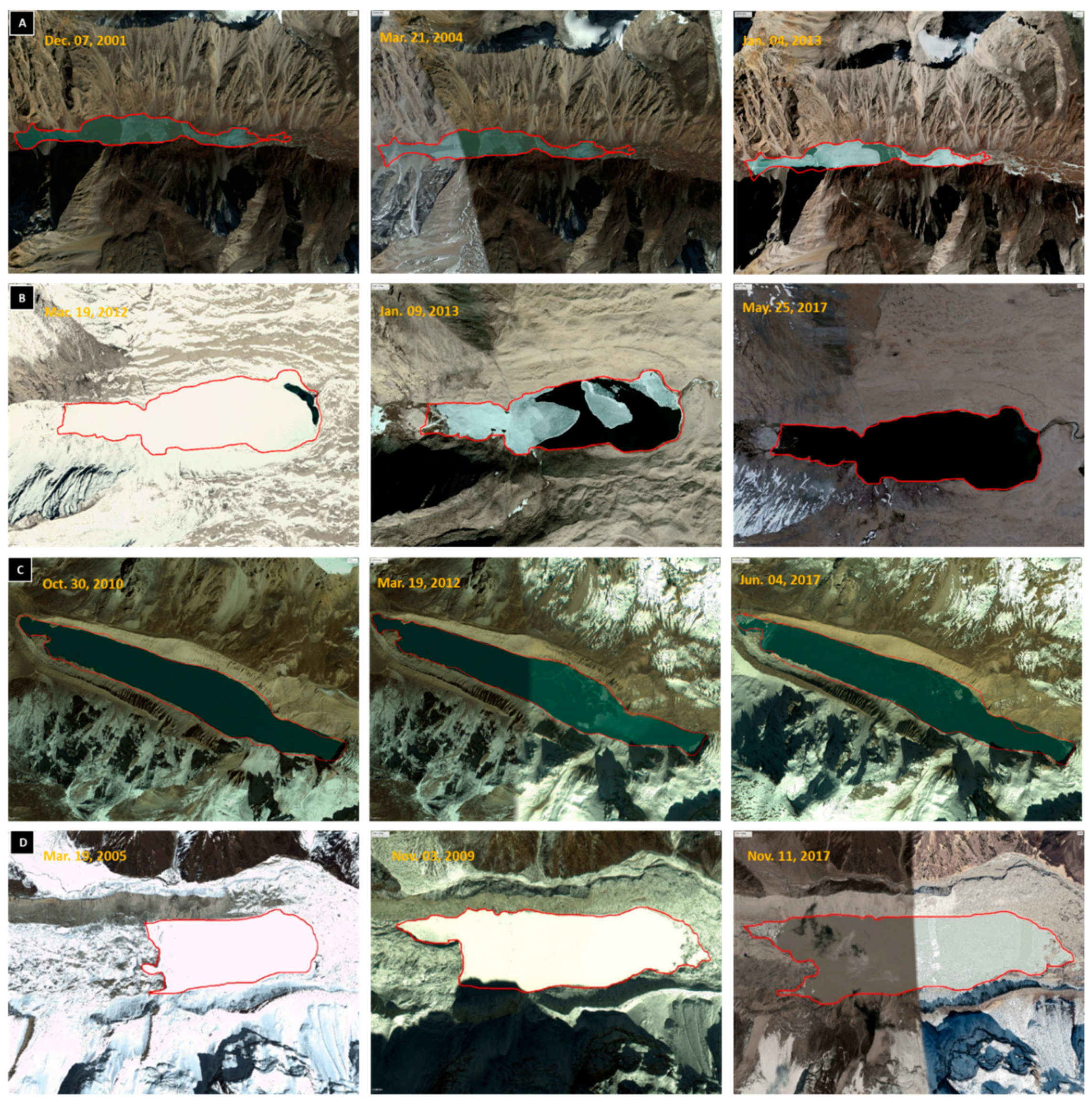
Glacial lake change in area profile during the period 2005–2017, where (a), (b), (c), and (d) represent lake nos. 20, 35, 36, and 49, respectively (Source: Google Earth).
Figure A3.
Glacial lake change in area profile during the period 2005–2017, where (a), (b), (c), and (d) represent lake nos. 20, 35, 36, and 49, respectively (Source: Google Earth).

Figure A4.
Critical change in area profile of glacial lakes during the period 1990–2018.

Figure A5.
Field investigation route from Kathmandu to Barun Khola.

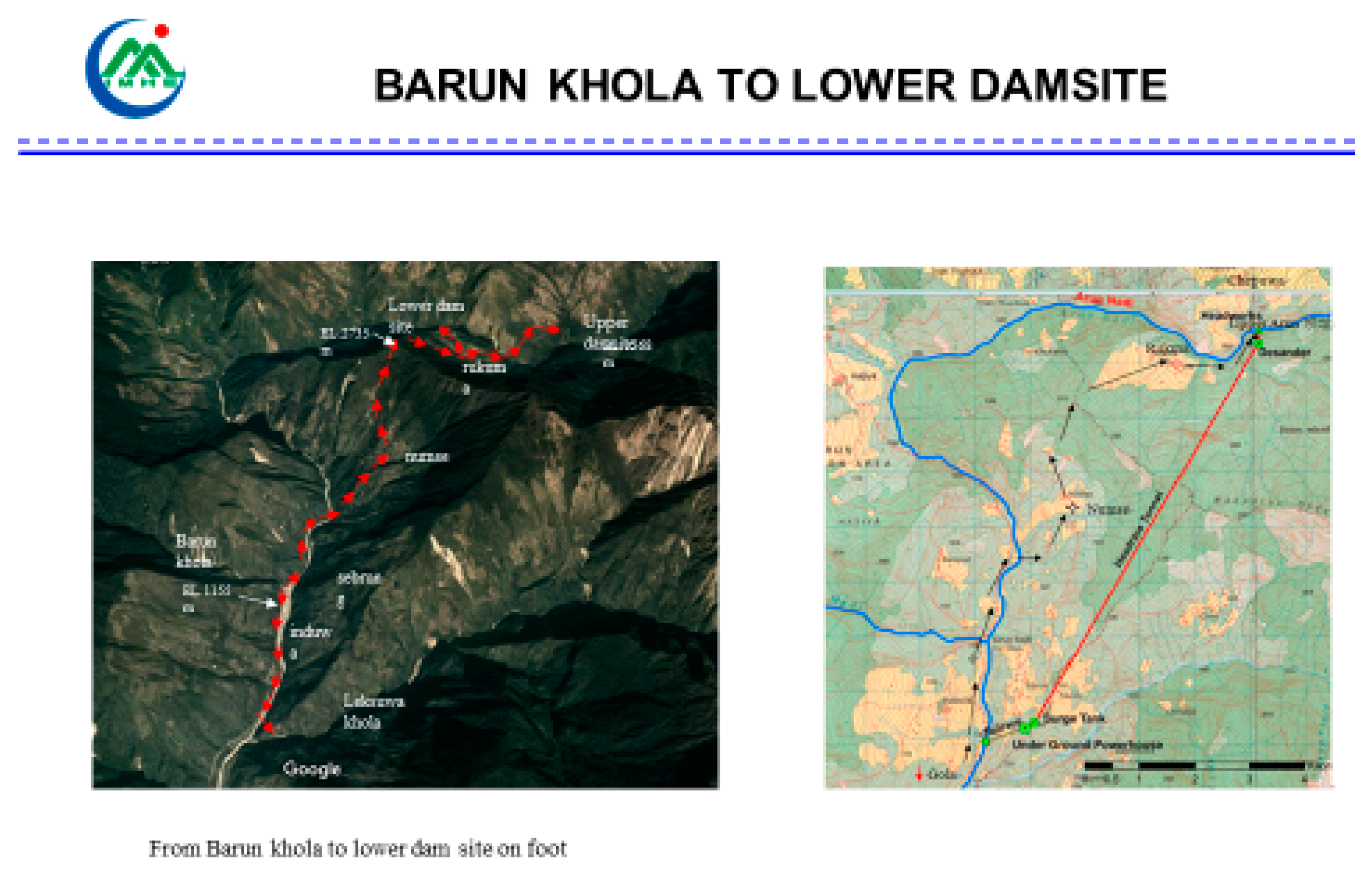
Figure A6.
Field investigation route from Barun Khola to lower dam site.

Figure A7.
Interview with the locals.

Figure A8.
Field activities at the lower dam site.

References
- Nie, Y.; Liu, Q.; Wang, J.; Zhang, Y.; Sheng, Y.; Liu, S. An inventory of historical glacial lake outburst floods in the Himalayas based on remote sensing observations and geomorphological analysis. Geomorphology 2018, 308, 91–106. [Google Scholar] [CrossRef]
- Bajracharya, S.R.; Mool, P. Glaciers, glacial lakes and glacial lake outburst floods in the Mount Everest region, Nepal. Ann. Glaciol. 2009, 50, 81–86. [Google Scholar] [CrossRef] [Green Version]
- Ives, D.J.; Shrestha, R.B.; Mool, P.K. Formation of Glacial Lakes in the Hindu Kush-Himalayas and GLOF Risk Assessment; ICIMOD: Kathmandu, Nepal, 2010. [Google Scholar]
- Wang, S.-J.; Zhang, T. Glacial lakes change and current status in the central Chinese Himalayas from 1990 to 2010. J. Appl. Remote. Sens. 2013, 7, 73459. [Google Scholar] [CrossRef]
- Chen, X.-Q.; Cui, P.; Li, Y.; Yang, Z.; Qi, Y.-Q. Changes in glacial lakes and glaciers of post-1986 in the Poiqu River basin, Nyalam, Xizang (Tibet). Geomorphology 2007, 88, 298–311. [Google Scholar] [CrossRef]
- Wang, W.; Gao, Y.; Anacona, P.I.; Lei, Y.; Xiang, Y.; Zhang, G.; Li, S.; Lu, A. Integrated hazard assessment of Cirenmaco glacial lake in Zhangzangbo valley, Central Himalayas. Geomorphology 2018, 306, 292–305. [Google Scholar] [CrossRef]
- Xu, D.; Feng, Q. Dangerous glacial lakes in the Himalayas of Tibet and their bursting characteristics. J. Geogr. Sci. 1989, 3, 343–352. [Google Scholar]
- Richardson, S.D.; Reynolds, J.M. An overview of glacial hazards in the Himalayas. Quat. Int. 2000, 65, 31–47. [Google Scholar] [CrossRef]
- Bajracharya, B.; Shrestha, A.B.; Rajbhandari, L. Glacial Lake Outburst Floods in the Sagarmatha Region. Mt. Res. Dev. 2007, 27, 336–344. [Google Scholar] [CrossRef]
- ICIMOD. Glacial Lakes and Glacial Lake Outburst Floods in Nepal; International Centre for Integrated Mountain Development: Lalitpur, Nepal, 2011. [Google Scholar]
- Osti, R.; Bhattarai, T.N.; Miyake, K. Causes of catastrophic failure of Tam Pokhari moraine dam in the Mt. Everest region. Nat. Hazards 2011, 58, 1209–1223. [Google Scholar] [CrossRef]
- Liu, J.-J.; Cheng, Z.-L.; Su, P.-C. The relationship between air temperature fluctuation and Glacial Lake Outburst Floods in Tibet, China. Quat. Int. 2014, 321, 78–87. [Google Scholar] [CrossRef]
- Gurung, D.R.; Khanal, N.R.; Bajracharya, S.R.; Tsering, K.; Joshi, S.; Tshering, P.; Chhetri, L.K.; Lotay, Y.; Penjor, T. Lemthang Tsho glacial Lake outburst flood (GLOF) in Bhutan: Cause and impact. Geoenviron. Disasters 2017, 4, 17. [Google Scholar] [CrossRef]
- Wang, W.; Yao, T.; Yang, X. Variations of glacial lakes and glaciers in the Boshula mountain range, southeast Tibet, from the 1970s to 2009. Ann. Glaciol. 2011, 52, 9–17. [Google Scholar] [CrossRef] [Green Version]
- Climate Change Secretariat. Impacts, Vulnerabilities and Adaptation in Developing Countries; Climate Change Secretariat (UNFCCC): Geneva, Switzerland, 2007. [Google Scholar]
- Wang, X.; Liu, S.; Ding, Y.; Guo, W.; Jiang, Z.; Lin, J.; Han, Y. An approach for estimating the breach probabilities of moraine-dammed lakes in the Chinese Himalayas using remote-sensing data. Nat. Hazards Earth Syst. Sci. 2012, 12, 3109–3122. [Google Scholar] [CrossRef] [Green Version]
- Che, T.; Jin, R.; Li, X.; Wu, L.Z. Glacial lakes variation and the potentially dangerous glacial lakes in the Pumqu Basin of Tibet during the last two decades. J. Glaciol. Geocryol. 2004, 26, 397–402. [Google Scholar]
- Bolch, T.; Peters, J.; Yegorov, A.; Pradhan, B.; Buchroithner, M.; Blagoveshchensky, V. Identification of potentially dangerous glacial lakes in the northern Tien Shan. Nat. Hazards 2011, 59, 1691–1714. [Google Scholar] [CrossRef] [Green Version]
- Gruber, F.E.; Mergili, M. Regional-scale analysis of high-mountain multi-hazard and risk indicators in the Pamir (Tajikistan) with GRASS GIS. Nat. Hazards Earth Syst. Sci. 2013, 13, 2779–2796. [Google Scholar] [CrossRef] [Green Version]
- Mergili, M.; Schneider, J.F. Regional-scale analysis of lake outburst hazards in the southwestern Pamir, Tajikistan, based on remote sensing and GIS. Nat. Hazards Earth Syst. Sci. 2011, 11, 1447–1462. [Google Scholar] [CrossRef] [Green Version]
- Wang, W.; Yao, T.; Gao, Y.; Yang, X.; Kattel, D.B. A First-order Method to Identify Potentially Dangerous Glacial Lakes in a Region of the Southeastern Tibetan Plateau. Mt. Res. Dev. 2011, 31, 122–130. [Google Scholar] [CrossRef]
- Emmer, A.; Vilímek, V. Review Article: Lake and breach hazard assessment for moraine-dammed lakes: An example from the Cordillera Blanca (Peru). Nat. Hazards Earth Syst. Sci. 2013, 13, 1551–1565. [Google Scholar] [CrossRef]
- Westoby, M.; Glasser, N.; Brasington, J.; Hambrey, M.; Quincey, D.; Reynolds, J. Modelling outburst floods from moraine-dammed glacial lakes. Earth Sci. Rev. 2014, 134, 137–159. [Google Scholar] [CrossRef] [Green Version]
- Worni, R.; Huggel, C.; Stoffel, M. Glacial lakes in the Indian Himalayas—From an area-wide glacial lake inventory to on-site and modeling based risk assessment of critical glacial lakes. Sci. Total Environ. 2013, 468, S71–S84. [Google Scholar] [CrossRef] [PubMed]
- Emmer, A.; Cochachin, A. The causes and mechanisms of moraine-dammed lake failures in the Cordillera Blanca, North American Cordillera, and Himalayas. AUC Geogr. 2013, 48, 5–15. [Google Scholar] [CrossRef] [Green Version]
- Nie, Y.; Liu, Q.; Liu, S. Glacial Lake Expansion in the Central Himalayas by Landsat Images, 1990–2010. PLoS ONE 2013, 8, 83973. [Google Scholar] [CrossRef] [PubMed]
- Raup, B.H.; Cogley, G.; Zemp, M.; Glaus, L. Recent Advances in the GLIMS Glacier Database. In AGU Fall Meeting Abstracts, Proceedings of the AGU Fall Meeting, San Francisco, CA, USA, 12–16 December 2016; American Geophysical Union: Washington, DC, USA, 2016. [Google Scholar]
- Bajracharya, S. GLIMS Glacier Database: Boulder; Colorado, National Snow and Ice Data Center/World Data Center for Glaciology: Boulder, CO, USA, 2008. [Google Scholar]
- Xu, D.M.; Feng, Q. Dangerous glacial lake and outburst features in Xizang Himalayas. Acta Geogr. Sin. 1989, 44, 343–352. [Google Scholar]
- Vuichard, D.; Zimmermann, M. The 1985 Catastrophic Drainage of a Moraine-Dammed Lake, Khumbu Himal, Nepal: Cause and Consequences. Mt. Res. Dev. 1987, 7, 91. [Google Scholar] [CrossRef]
- Osti, R.; Egashira, S. Hydrodynamic characteristics of the Tam Pokhari Glacial Lake outburst flood in the Mt. Everest region, Nepal. Hydrol. Process. Int. J. 2009, 23, 2943–2955. [Google Scholar] [CrossRef]
- Dwivedi, S.K. The Tam Pokhari glacier lake outburst flood of 3 September 1998. J. Nepal Geol. Soc. 2000, 22, 539–546. [Google Scholar]
- Mool, P.K.; Wangda, D.; Bajracharya, S.R.; Joshi, S.P.; Kunzang, K.; Gurung, D.R. Inventory of Glaciers, Glacial Lakes and Glacial Lake Outburst Floods: Monitoring and Early Warning Systems in the Hindu Kush-Himalayan Region, Nepal; ICIMOD: Kathmandu, Nepal, 2001. [Google Scholar]
- Popov, N. Assessment of glacial debris flow hazard in the north Tien-Shan. In Proceedings of the Soviet-China-Japan Symposium and Field Workshop on Natural Disasters; Alma-ata: Shanghai, China; Dushanbe and Kazselezashchita: Lanzhou, China; USSR: Urumgi, China, 1991; pp. 384–391. [Google Scholar]
- Evans, S.G. The maximum discharge of outburst floods caused by the breaching of man-made and natural dams. Can. Geotech. J. 1986, 23, 385–387. [Google Scholar] [CrossRef]
- O’Connor, J.E.; Walder, J.S. Methods for predicting peak discharge of floods caused by failure of natural and constructed earthen dams. Water Resour. Res. 1997, 33, 2337–2348. [Google Scholar]
- Haeberli, W.; Teysseire, P.; Huggel, C.; Kääb, A.; Paul, F. Remote sensing based assessment of hazards from glacier lake outbursts: A case study in the Swiss Alps. Can. Geotech. J. 2002, 39, 316–330. [Google Scholar]
- Fan, X.; Tang, C.X.; Van Westen, C.J.; Alkema, D. Simulating dam-breach flood scenarios of the Tangjiashan landslide dam induced by the Wenchuan Earthquake. Nat. Hazards Earth Syst. Sci. 2012, 12, 3031–3044. [Google Scholar] [CrossRef] [Green Version]
- Veh, G.; Korup, O.; von Specht, S.; Roessner, S.; Walz, A. Unchanged frequency of moraine-dammed glacial lake outburst floods in the Himalaya. Nat. Clim. Chang. 2019, 9, 379–383. [Google Scholar] [CrossRef]
- Wang, W.; Xiang, Y.; Gao, Y.; Lu, A.; Yao, T. Rapid expansion of glacial lakes caused by climate and glacier retreat in the Central Himalayas. Hydrol. Process. An Int. J. 2015, 29, 859–874. [Google Scholar] [CrossRef]
- Bajracharya, S.R.; Mool, P.K.; Shrestha, B.R. Impact of Climate Change on Himalayan Glaciers and Glacial Lakes: Case Studies on GLOF and Associated Hazards in Nepal and Bhutan; International Centre for Integrated Mountain Development (ICIMOD): Lalitpur, Nepal, 2007. [Google Scholar]
Figure 1.
The study area.

Figure 2.
Methodology.

Figure 3.
Remote sensing using satellite images to identify glaciers and glacial lakes for the years (A) 1990, (B) 1995, (C) 2000, (D) 2005, (E) 2011, and (F) 2018.
Figure 3.
Remote sensing using satellite images to identify glaciers and glacial lakes for the years (A) 1990, (B) 1995, (C) 2000, (D) 2005, (E) 2011, and (F) 2018.

Figure 4.
Lake volume versus affected length of historical GLOFs.

Figure 5.
Locations of glaciers, glacial lakes with areas greater than 0.1 km2, and potentially critical glacial lakes (nos. 20, 35, 36, and 49) and their outburst paths.
Figure 5.
Locations of glaciers, glacial lakes with areas greater than 0.1 km2, and potentially critical glacial lakes (nos. 20, 35, 36, and 49) and their outburst paths.

Figure 6.
Discharge profiles of lake nos. 20, 35, 36, and 39 in (a–d), respectively, from the outburst site to the downstream.
Figure 6.
Discharge profiles of lake nos. 20, 35, 36, and 39 in (a–d), respectively, from the outburst site to the downstream.

Figure 7.
Discharge profiles of lake nos. 20, 35, 36, and 39 with 100%, 75%, and 50% drainage in (a)–(d), respectively, from the outburst site to the downstream region.
Figure 7.
Discharge profiles of lake nos. 20, 35, 36, and 39 with 100%, 75%, and 50% drainage in (a)–(d), respectively, from the outburst site to the downstream region.

Figure 8.
(a) Correlation among precipitation, temperature, and GLOF events during 1935–2017. (b) Seasonal annual average variation in precipitation during 1960–2017. (c) Seasonal annual average variation in temperature during 1960–2017.
Figure 8.
(a) Correlation among precipitation, temperature, and GLOF events during 1935–2017. (b) Seasonal annual average variation in precipitation during 1960–2017. (c) Seasonal annual average variation in temperature during 1960–2017.

Figure 9.
Relationship between moraine lake area and average depth.


Table 1.
Volume and affected length of historical glacial lake outburst floods (GLOFs) that occurred in Nepal and Tibet (China).
Table 1.
Volume and affected length of historical glacial lake outburst floods (GLOFs) that occurred in Nepal and Tibet (China).
| No. | Name | Date | Volume V (× 106 m3) | Affected Length L (km) | Reference |
|---|---|---|---|---|---|
| 1 | Cirenmacuo | 11 July 1981 | 18.9 | 53 | [29] |
| 2 | Jialongco | 23 May 2002 | 3.9 | 46 | [29] |
| 3 | Taaco | 28 August 1935 | 6.3 | 30 | [29] |
| 4 | Qiongbixiamacuo | 10 July 1940 | 12.4 | 44 | [29] |
| 5 | Sangwang Lake | 16 July 1954 | 300 | 200 | [29] |
| 6 | Longdacuo | 25 August 1964 | 10.8 | 28 | [29] |
| 7 | Gelhaipuco | 21 September 1964 | 23.4 | 43 | [29] |
| 8 | Ayaco | 18 August 1970 | 90 | 42 | [29] |
| 9 | Dig Tsho | 4 August 1985 | 8 | 42 | [30] |
| 10 | Tam Pokhari | 3 September 1988 | 17.7 | 66 | [31,32,33] |
| 11 | Luggye Tsho | 7 October 1994 | 48 | 84 | [8] |
Table 2.
Annual variation in area, volume, calculated affected length (Lc), and distance between the lake and the dam site (Ld) and the Upper Arun powerhouse (Lp) for the 49 glacial lakes with areas > 0.1 km2 in the Arun River Basin for the period 1990–2017.
Table 2.
Annual variation in area, volume, calculated affected length (Lc), and distance between the lake and the dam site (Ld) and the Upper Arun powerhouse (Lp) for the 49 glacial lakes with areas > 0.1 km2 in the Arun River Basin for the period 1990–2017.
| No. | Location | Lake Area (km2) | Volume (106 m3) | Ld (km) | Lc (km) | Lp (km) | Lc/Lp | ||||||
|---|---|---|---|---|---|---|---|---|---|---|---|---|---|
| Longitude ( ) | Latitude ( ) | 1990 | 1995 | 2000 | 2005 | 2011 | 2017 | ||||||
| 1 | 86.305 | 28.374 | 3.641 | 3.727 | 3.727 | 3.692 | 3.762 | 3.867 | 212.685 | 232.190 | 169.810 | 248.370 | 0.680 |
| 2 | 86.379 | 28.392 | 0.327 | 0.410 | 0.613 | 0.750 | 0.903 | 1.093 | 60.115 | 227.220 | 90.470 | 243.400 | 0.370 |
| 3 | 86.415 | 28.393 | 0.177 | 0.177 | 0.188 | 0.188 | 0.181 | 0.181 | 9.955 | 226.140 | 64.390 | 242.320 | 0.270 |
| 4 | 86.494 | 28.349 | 0.294 | 0.294 | 0.294 | 0.294 | 0.294 | 0.294 | 16.170 | 222.570 | 67.620 | 238.750 | 0.280 |
| 5 | 86.582 | 28.199 | 1.330 | 1.330 | 1.330 | 1.330 | 1.287 | 1.274 | 70.070 | 183.600 | 95.650 | 199.780 | 0.480 |
| 6 | 86.629 | 28.207 | 0.268 | 0.268 | 0.268 | 0.268 | 0.268 | 0.268 | 14.740 | 185.890 | 66.870 | 202.070 | 0.330 |
| 7 | 86.863 | 28.111 | 0.015 | 0.098 | 0.098 | 0.098 | 0.312 | 0.388 | 21.340 | 154.050 | 70.310 | 170.230 | 0.410 |
| 8 | 87.028 | 28.008 | 0.103 | 0.103 | 0.103 | 0.103 | 0.103 | 0.103 | 5.665 | 68.360 | 62.160 | 84.540 | 0.740 |
| 9 | 87.047 | 28.068 | 0.543 | 0.574 | 0.574 | 0.630 | 0.707 | 0.745 | 40.975 | 86.570 | 80.520 | 102.750 | 0.780 |
| 10 | 87.051 | 28.206 | 0.626 | 0.626 | 0.573 | 0.573 | 0.573 | 0.573 | 31.515 | 89.910 | 75.600 | 106.090 | 0.710 |
| 11 | 87.082 | 27.844 | 0.294 | 0.294 | 0.294 | 0.325 | 0.340 | 0.345 | 18.975 | 39.570 | 69.080 | 39.570 | 1.750 |
| 12 | 87.082 | 28.130 | 0.177 | 0.177 | 0.177 | 0.177 | 0.177 | 0.177 | 9.735 | 85.520 | 64.270 | 101.700 | 0.630 |
| 13 | 87.101 | 28.208 | 0.937 | 0.937 | 0.937 | 0.937 | 0.937 | 0.937 | 51.535 | 84.230 | 86.010 | 100.410 | 0.860 |
| 14 | 87.105 | 28.143 | 0.146 | 0.146 | 0.146 | 0.146 | 0.146 | 0.146 | 8.030 | 82.330 | 63.390 | 98.510 | 0.640 |
| 15 | 87.112 | 28.143 | 0.217 | 0.217 | 0.217 | 0.217 | 0.217 | 0.217 | 11.935 | 81.610 | 65.420 | 97.790 | 0.670 |
| 16 | 87.134 | 28.069 | 0.201 | 0.201 | 0.201 | 0.201 | 0.201 | 0.201 | 11.055 | 78.140 | 64.960 | 94.320 | 0.690 |
| 17 | 87.428 | 28.138 | 0.211 | 0.211 | 0.211 | 0.211 | 0.211 | 0.211 | 11.605 | 65.420 | 65.240 | 81.600 | 0.800 |
| 18 | 87.443 | 28.161 | 0.222 | 0.222 | 0.243 | 0.214 | 0.239 | 0.224 | 12.320 | 73.010 | 65.620 | 89.190 | 0.740 |
| 19 | 87.468 | 28.149 | 0.255 | 0.255 | 0.255 | 0.255 | 0.255 | 0.255 | 14.025 | 76.260 | 66.500 | 92.440 | 0.720 |
| 20 | 87.472 | 28.213 | 1.025 | 1.025 | 1.137 | 1.319 | 1.319 | 1.319 | 72.545 | 83.280 | 96.930 | 99.460 | 0.970 |
| 21 | 87.480 | 28.173 | 0.208 | 0.208 | 0.208 | 0.208 | 0.208 | 0.208 | 11.440 | 77.290 | 65.160 | 93.470 | 0.700 |
| 22 | 87.502 | 28.237 | 0.166 | 0.166 | 0.166 | 0.166 | 0.166 | 0.166 | 9.130 | 87.290 | 63.960 | 103.470 | 0.620 |
| 23 | 87.563 | 28.179 | 0.691 | 0.803 | 0.840 | 0.885 | 0.989 | 1.013 | 55.715 | 94.610 | 88.180 | 110.790 | 0.800 |
| 24 | 87.578 | 28.228 | 0.190 | 0.190 | 0.190 | 0.190 | 0.190 | 0.190 | 10.450 | 106.750 | 64.640 | 122.930 | 0.530 |
| 25 | 87.578 | 28.164 | 0.171 | 0.180 | 0.180 | 0.180 | 0.180 | 0.180 | 9.900 | 76.350 | 64.360 | 92.530 | 0.700 |
| 26 | 87.584 | 28.107 | 0.117 | 0.117 | 0.117 | 0.117 | 0.117 | 0.117 | 6.435 | 71.840 | 62.560 | 88.020 | 0.710 |
| 27 | 87.587 | 28.116 | 0.105 | 0.105 | 0.105 | 0.105 | 0.105 | 0.105 | 5.775 | 72.190 | 62.210 | 88.370 | 0.700 |
| 28 | 87.591 | 28.230 | 0.719 | 0.786 | 0.786 | 0.768 | 0.786 | 0.745 | 40.975 | 107.770 | 80.520 | 123.950 | 0.650 |
| 29 | 87.599 | 28.131 | 0.122 | 0.122 | 0.122 | 0.122 | 0.122 | 0.122 | 6.710 | 80.030 | 62.700 | 96.210 | 0.650 |
| 30 | 87.612 | 28.155 | 0.127 | 0.127 | 0.127 | 0.127 | 0.127 | 0.127 | 6.985 | 80.230 | 62.840 | 96.410 | 0.650 |
| 31 | 87.615 | 28.118 | 0.241 | 0.241 | 0.241 | 0.241 | 0.241 | 0.241 | 13.255 | 77.860 | 66.100 | 94.040 | 0.700 |
| 32 | 87.623 | 28.168 | 0.200 | 0.200 | 0.200 | 0.200 | 0.200 | 0.200 | 11.000 | 84.210 | 64.930 | 100.390 | 0.650 |
| 33 | 87.637 | 28.093 | 0.377 | 0.377 | 0.525 | 0.564 | 0.588 | 0.588 | 32.340 | 72.820 | 76.030 | 89.000 | 0.850 |
| 34 | 87.641 | 28.195 | 0.497 | 0.497 | 0.497 | 0.497 | 0.497 | 0.497 | 27.335 | 94.830 | 73.420 | 111.010 | 0.660 |
| 35 | 87.655 | 28.114 | 1.289 | 1.268 | 1.268 | 1.268 | 1.268 | 1.268 | 69.740 | 73.330 | 95.470 | 89.510 | 1.070 |
| 36 | 87.772 | 27.926 | 0.636 | 0.767 | 0.767 | 0.794 | 0.857 | 0.857 | 47.135 | 60.830 | 83.720 | 77.010 | 1.090 |
| 37 | 87.815 | 27.964 | 0.175 | 0.230 | 0.230 | 0.342 | 0.342 | 0.342 | 18.810 | 71.180 | 68.990 | 87.360 | 0.790 |
| 38 | 87.908 | 27.952 | 0.663 | 0.663 | 0.663 | 0.632 | 0.632 | 0.632 | 34.760 | 82.190 | 77.290 | 98.370 | 0.790 |
| 39 | 87.931 | 27.950 | 0.597 | 0.597 | 0.679 | 0.745 | 0.745 | 0.745 | 40.975 | 83.730 | 80.520 | 99.910 | 0.810 |
| 40 | 88.003 | 27.930 | 0.853 | 0.890 | 0.930 | 0.930 | 0.930 | 0.930 | 51.150 | 97.710 | 85.810 | 113.890 | 0.750 |
| 41 | 88.066 | 27.934 | 0.728 | 0.728 | 0.728 | 0.728 | 0.705 | 0.728 | 40.040 | 102.920 | 80.030 | 119.100 | 0.670 |
| 42 | 88.076 | 27.946 | 0.593 | 0.748 | 0.865 | 1.108 | 1.292 | 1.516 | 83.380 | 101.380 | 102.570 | 117.560 | 0.870 |
| 43 | 88.242 | 28.005 | 0.264 | 0.292 | 0.311 | 0.323 | 0.328 | 0.336 | 18.480 | 171.200 | 68.820 | 187.380 | 0.370 |
| 44 | 88.259 | 28.009 | 0.351 | 0.389 | 0.434 | 0.514 | 0.491 | 0.514 | 28.270 | 170.540 | 73.910 | 186.720 | 0.400 |
| 45 | 88.288 | 28.018 | 0.390 | 0.390 | 0.390 | 0.390 | 0.390 | 0.390 | 21.450 | 172.140 | 70.360 | 188.320 | 0.370 |
| 46 | 88.320 | 28.006 | 0.331 | 0.331 | 0.331 | 0.331 | 0.331 | 0.331 | 18.205 | 174.880 | 68.680 | 191.060 | 0.360 |
| 47 | 88.355 | 28.023 | 0.479 | 0.479 | 0.479 | 0.479 | 0.479 | 0.479 | 26.345 | 182.100 | 72.910 | 198.280 | 0.370 |
| 48 | 88.427 | 28.054 | 0.857 | 0.857 | 0.857 | 0.857 | 0.857 | 0.857 | 47.135 | 184.160 | 83.720 | 200.340 | 0.420 |
| 49 | 87.091 | 27.798 | 0.504 | 0.649 | 0.904 | 1.003 | 1.230 | 1.480 | 81.400 | 34.050 | 101.540 | 34.050 | 2.980 |
Note: Lake nos. 1–10 and 12–48 are located upstream of the dam site; lake nos. 11 and 49 are located downstream of the dam site.
Table 3.
Empirical formulas for calculating the peak discharge at the glacial lake dam site.
| Formula | Source | Note |
|---|---|---|
| [34] | Qm is the peak discharge at the dam site, and Vw is the volume of water. | |
| [35] | ||
| [36] | ||
| [37] |
Table 4.
Maximum discharge and physical features of the critical lakes.
| Glacial Lake No. | Discharge at Site if Drainage = | Dam Type | Potential for Lake Impacts | Dam Geometry | Freeboard | Outburst Probability | ||
|---|---|---|---|---|---|---|---|---|
| 100% | 75% | 50% | ||||||
| 20 | 4632 | 3542 | 2422 | Landslide dam | Debris flow | Stable | Medium freeboard | Medium |
| 35 | 4929 | 3772 | 2583 | No dam | Debris flow | - | Low freeboard | Medium |
| 36 | 3951 | 3025 | 2073 | Moraine dam | Ice avalanches/rock fall | Unstable | Low freeboard | High |
| 49 | 9866* | 7586* | 5238* | Moraine dam | Ice avalanches/rock fall | Unstable | Low freeboard | High |
* Discharge of lake no. 49 is at the powerhouse site, as it is located downstream of the dam site.
© 2019 by the authors. Licensee MDPI, Basel, Switzerland. This article is an open access article distributed under the terms and conditions of the Creative Commons Attribution (CC BY) license (http://creativecommons.org/licenses/by/4.0/).
Share and Cite
MDPI and ACS Style
Washakh, R.M.A.; Chen, N.; Wang, T.; Almas, S.; Ahmad, S.R.; Rahman, M. GLOF Risk Assessment Model in the Himalayas: A Case Study of a Hydropower Project in the Upper Arun River. Water 2019, 11, 1839. https://doi.org/10.3390/w11091839
AMA Style
Washakh RMA, Chen N, Wang T, Almas S, Ahmad SR, Rahman M. GLOF Risk Assessment Model in the Himalayas: A Case Study of a Hydropower Project in the Upper Arun River. Water. 2019; 11(9):1839. https://doi.org/10.3390/w11091839
Chicago/Turabian StyleWashakh, Rana Muhammad Ali, Ningsheng Chen, Tao Wang, Sundas Almas, Sajid Rashid Ahmad, and Mahfuzur Rahman. 2019. "GLOF Risk Assessment Model in the Himalayas: A Case Study of a Hydropower Project in the Upper Arun River" Water 11, no. 9: 1839. https://doi.org/10.3390/w11091839
Note that from the first issue of 2016, this journal uses article numbers instead of page numbers. See further details here.