Water-Energy Nexus for an Italian Storage Hydropower Plant under Multiple Drivers
by
 ,
,
Mattia Bonato
1, 
Alessandro Ranzani
1,
Epari Ritesh Patro
1,*,
Ludovic Gaudard
2 and
Carlo De Michele
1,* 1
Department of Civil and Environmental Engineering, Politecnico di Milano, 20133 Milan, Italy
2
Department of Management Science and Engineering, Stanford University, Stanford, CA 94305, USA
*
Authors to whom correspondence should be addressed.
Water 2019, 11(9), 1838; https://doi.org/10.3390/w11091838
Submission received: 9 August 2019
/
Revised: 28 August 2019
/
Accepted: 1 September 2019
/
Published: 4 September 2019
(This article belongs to the Section Water, Agriculture and Aquaculture)
Abstract
:Climate change has repercussions on the management of water resources. Particularly, changes in precipitation and temperature impact hydropower generation and revenue by affecting seasonal electricity prices and streamflow. This issue exemplifies the impact of climate change on the water-energy-nexus, which has raised serious concern. This paper investigates the impact of climate change on hydropower with a multidisciplinary approach. A holistic perspective should be favored as the issue is complex, consequently, we chose to investigate a specific case study in Italy. It allows grasping the details, which matters in mountainous area. We integrated a hydrological model, hydropower management model, nine climate scenarios, and five electricity scenarios for a specific storage hydropower plant. Independently from the scenarios, the results show a glacier volume shrinkage upward of 40% by 2031 and minimum of 50% by 2046. The reservoir mitigates losses of revenue that reach 8% in the worst case, however, are lower compared with run-of-the-river configuration. Changes in price seasonality amplitude also determine modifications in revenues, while temporal shifts appear to be ineffective. For run-of-the-river, any variation in hydrological cycle immediately translates into revenue. Comparing the results of all future scenarios with the base scenario, it can be concluded that an increase in temperature will slightly improve the performances of hydropower.
1. Introduction
Hydropower has a great importance in global electricity generation, representing the 15% of the worldwide amount [1], and accounting for the 85% of the total production [2] in the world’s renewable energy framework. This technology has the great advantage of ensuring operational flexibility and enhancing the possibility of storing energy and managing the production. It increases the reliability of the electric system, acting as an ancillary service. This is a fundamental characteristic especially with the increasing development of intermittent sources like wind and photovoltaic [3,4,5,6].
For these reasons, increasing attention has been lately posed on the quantification of the effects of climate changes on hydropower [7], considering increase in temperature or change in temporal and spatial patterns of liquid and solid precipitation [8,9]. Due to its strong dependency on hydrologic regime, hydropower is among the most vulnerable technologies to climate changes [10]. In addition, as the production of this power source relies not only on inflows but also on electricity prices [11], it becomes important to understand how climate changes will affect these two drivers.
Precipitation and glacier volume will change. In mountainous areas, one can expect a progressive decrease in peak snow accumulation [12,13,14]. Laternser and Schneebeli [12] have shown a decrement in seasonal snow depth starting from the mid 80s, a trend confirmed in all the northern hemisphere by various studies [15,16,17] and more evident at lower elevations. In addition, several hydropower plants are built downstream from glaciers, whose shrinkage has been deeply demonstrated in existing literature [18,19,20]. Cat Berro et al. [21] showed the total Alpine glacier area reduced from about 4500 km2 in 1850 to the 2270 km2 in 2000. Analyzing the Sforzellina glacier in Valfurva (Italy), Cannone et al. [22] found an area reduction of 36% in the time interval 1981–2006, with an increase in the rate of depletion from −0.005 km2/y in the period 1981–2002 up to −0.0097 in the period 2002–2006. Diolaiuti et al. [23] found an area reduction of the 56% of the Dosdè-Piazzi glacier in Valtellina in the time interval 1954–2003, with a doubling of the rate in the last decades, from −0.058 km2/y for years between 1954 and 1981, to −0.145 km2/y in the period 1991–2003. A global warming of 2–4 °C by the end of this century would reduce 50%–90% of the Alpine ice mass [11,24].
These evolutions will impact runoff volumes and seasonality. The shrinkage of glaciers will increase runoff at the near horizon due to meltwater, through the so-called peak water [18,25,26,27]. However, this effect would progressively disappear, leading to a net loss of available volume [28,29,30]. Moreover, change in climate patterns will affect seasonality of streamflows, particularly in snow- or ice-dominated catchments. Warming will shift the beginning of snowmelt [28] or glacier melt. Combined with a modification in precipitation patterns, inter-annual runoff will vary, leading to an increase of water in winter and a decrease in summer [31,32].
Climate changes are also expected to influence power market [33], as electricity is linked to weather variables [34]. Temperature and humidity influence consumption, production, and transmission, thus demand, supply, and prices [33]. Seasonal cycles of demand may change, with an increase in summer and a decrease in winter [35]. The risk of seasonal mismatches between electricity supply and demand/price is increasing due to expanded use of wind, solar, hydropower, and other renewable energy sources. All these effects are expected to have an impact on electricity prices and their seasonality.
Sustainable use of energy and water in a hydropower context is fundamental in its environmental, economic, and social dimensions [26,36,37]. The existing literature contains may studies separately analyzing the impacts of climate changes on electricity market [38,39,40], on runoff [14,18,20,25,41], and on price and inflows seasonality [42]. However, the “water-energy-nexus” has been generally studied as independent variables [43,44]. Madani et al. [45] highlighted the necessity of investigating the two drivers together. Some works tried to fill this gap, considering the future perspectives of catchments dominated by storage hydropower plants [42,45,46,47]. Nevertheless, the investigation of seasonality is limited. It was tackled in Gaudard et al. [26] but for a run-of-river hydropower plant, which discards an important aspect related to water management. To anticipate and mitigate the impact of climate change, it becomes urgent to investigate the issue with a multidisciplinary perspective, a fine time resolution, and including management options.
This research contributes to this effort by investigating a specific case study. It allows going deeper into details and grasping the complexity of the issue. We consider an Italian ice-dominated catchment and combine economics and hydrology at an hourly time scale. Beside change of seasonality due to climate change, five electricity price seasonality scenarios are considered [26]. The originality of the present work resides in the fact that a multidisciplinary and multi-model approach has been applied, as economic and climatic evolutions are modelled. Another originality is in the procedure adopted in the definition of price and climate scenarios. The novelty of the paper lies in the assessment of future hydropower availabilities of a storage plant and comparison with the run-of-the-river mode. This work aimed to contribute to enhancing a clear and simple understanding of the results and an intuitive assessment of future management strategies adopted, representing a good benchmark for decision makers.
2. Italian Hydropower: Current Situation and Climate Change Impact Projections
With 18.8 GW installed hydropower capacity in 2017, Italy is ranked 11th at the global level and 4th at the European scale [48]. A total of 53.3 GW of electricity is from renewables accounting to 35% of Italian energy mix, where hydropower accounts for 35% of the renewable energy produced [49,50]. Hydropower is strategic since Italy conceals a minimum amount of fossil feedstock and depends on resources from abroad [51]. As of 2016, the import of fossil fuels accounted for 92.6% [52]. In the Italian framework, the National Electricity Strategy (Strategia Elettrica Nazionale, in Italian) [53] and the recent Integrated National Plan for Energy and Climate (Piano Nazionale Integrato per l’Energia e il Clima, in Italian) [54] fix future national energy policies, depicting future pathways in renewable sources sector. They target a progressive phase out of generation from coal by 2025, and 55.4% of national electricity consumption from renewable energy sources (RES) by 2030 [55]. To achieve this goal, new incentivizing policies must double or even triple wind and solar energy at 2030, throughout new constructions as well as revamping and repowering existing installations. It will ask for increasing storage capacity to manage intermittent supply. This will empower the sharing of existing and the building of new pump-and-storage power plants. It nowadays represents the most mature storage technologies, despite new incomers are becoming competitive [56]. In terms of energy generation, the exploitable hydropower potential is becoming scare. It, nevertheless, represents a strategic asset in baseload and peak-load generation. Therefore, the Italian Ministry of Economic Development (Ministero dello Sviluppo Economico) aims at incentivizing the revamping of existing “great hydropower” rather than the construction of new hydropower, with the exception of only “small hydropower plants” (i.e., SHP) [53,54].
The 4268 hydropower plants are heterogeneously spread throughout the country [49]. Small installations are numerous: 3074 (≤1 MW), 886 (1–10 MW). However, the remaining 308 (>10 MW) plants contribute to 75% of the total hydroelectric power generated [49]. Therefore, Northern part of Italy regroups 81.8% of the installations and 59.5% of installed capacity (see Table 1). Following the latest report of the Italian Regulatory Authority [57] the share of hydropower managed by major companies is as such, Enel (37.7%), A2A (9.9%), Erg (3.2%), Edison (5.3%), CVA (6.3%), Hydro Dolomiti Energia (6%), Alperia (4.6%), SEL (4.2%), Iren (2.9%), and others (20.8%). Whereas in central and southern Italy, Abruzzo and Calabria have the maximum hydropower concentration in terms of energy generation.
The streamflow regime of Italian hydropower is typically of two types: (a) snow and/or glacier dominated (low flow in winter while high flow in spring and summer); (b) rainfall dominated (depends on the seasonality of rainfall, typically low flow during summer) [18,26]. With the anticipated changes in climate due to global warming, substantial changes are expected for streamflow of snow and/or glacier dominated hydropower catchment [7,58]. With the retreat of glaciers a temporary increase in streamflow is expected for the near future and is completely dependent on the characteristic of the catchment and rate of climate change; with a possibility of change in the regime of hydropower catchment from glacier to snow or snow to rainfall based [18,59]. For mountain catchments, particularly in the Alpine region these shifts in hydrological regime is due to the early onset of melting season and shrinkage of glaciers, resulting in higher streamflow in early summer and spring [18,20,60,61,62]. In the recent work of Smiraglia et al. [63], the area changes in Italian glaciers in the New Italian Glacier Inventory [64] are compared with both the CGI-CNR Inventory [65] and WGI (World Glacier Inventory) dataset. They observed a change of −30% and −39% respectively in the last five decades. It is therefore necessary to understand the influence of climate change in the Italian hydropower sector. Table 2 gives some insights on the studies conducted in this decade for possible consequences of climate change on Italian hydropower.
Assessment and quantification of climate change impacts on hydropower are quite complex in nature [7,66]. From the existing literature reported in Table 2, it is clear that the implications are site specific depending on the catchment and use of hydropower apart from power generation (e.g., drinking, recreational, irrigation). The evaluation of hydropower at both a regional and national level is quite tiresome due to the need for detailed information such as meteorological variables, streamflow, design specification, inter-basin transfers, water usage among others. Therefore, most of the studies reported in Table 2 evaluate a single hydropower site. From these studies, it was observed for Italian hydropower a reduction in late summer flow and anticipation of peak streamflow for snow dominated catchments. For the comprehensive overview of projected changes refer to Table 2.
3. Methodology and Case Study
This section presents the models and dataset utilized to build the analysis on a case study, along with the workflow adopted. The hydrological and hydropower management model are described along with the future scenarios of climate and electricity price used for simulations. Finally, the case study will be presented, describing in detail the main features of the basin considered and the data available.
3.1. Study Area and Data
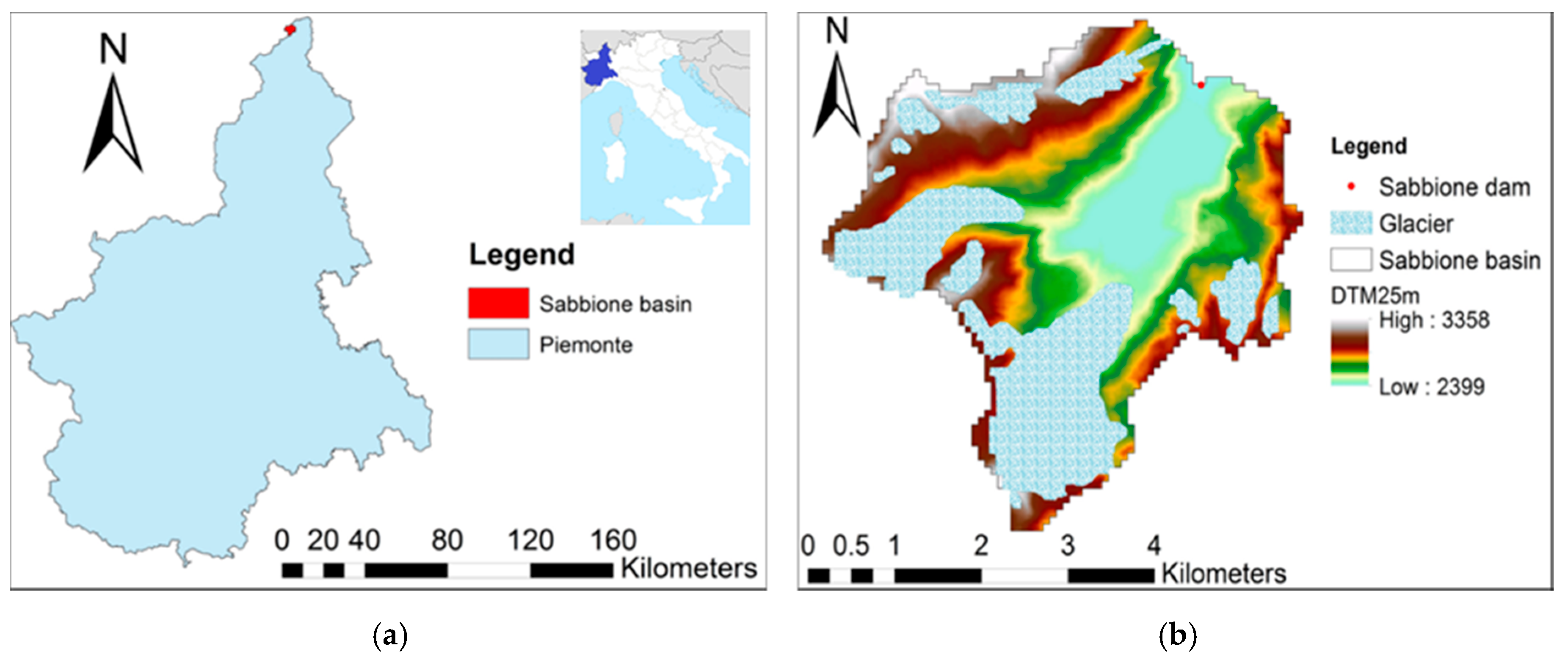
This paper focuses on the Sabbione catchment, located in Val d’Ossola, in the northern part of Piedmont region of Italy (see Figure 1a). The main feature of this catchment along with the hydropower plant considered as the closing section is presented in Table 3. The delimitation of the catchment was done considering the Sabbione dam (Morasco hydropower plant) as closure. This catchment has altitude range between 2460–3358 m above sea level (m.a.s.l), comprising four glaciers that cover approximately the 30% of the whole area of the catchment [64]. Recent work by Giaccone et al. [84] observes a glacier retreat in this catchment of 2 km in the time interval 1885–2011.
The hydropower plants originally built in the glacier valley used to encompass the front of the glacier submerged in Morasco hydropower’s reservoir before the glacier retreat. The Sabbione reservoir (see Table 3) is the biggest artificial reservoir of the Ossola and Piedmont Region, the second for dimensions in the whole alpine chain behind Place Moulin in Val d’Aosta [18]. Enel manages this reservoir and dam and exploits the water from snow, precipitation, and glacier fed Toce river basin. This catchment has been studied previously in the literature [11,18] predicting the hydropower future of this basin in terms of power production and glacier coverage only. However, the impact of climate change seasonality on the revenue was neglected. The reservoir is used for hydropower production only, since irrigation is not present and domestic water usage is negligible.
3.2. The Hydrological Model
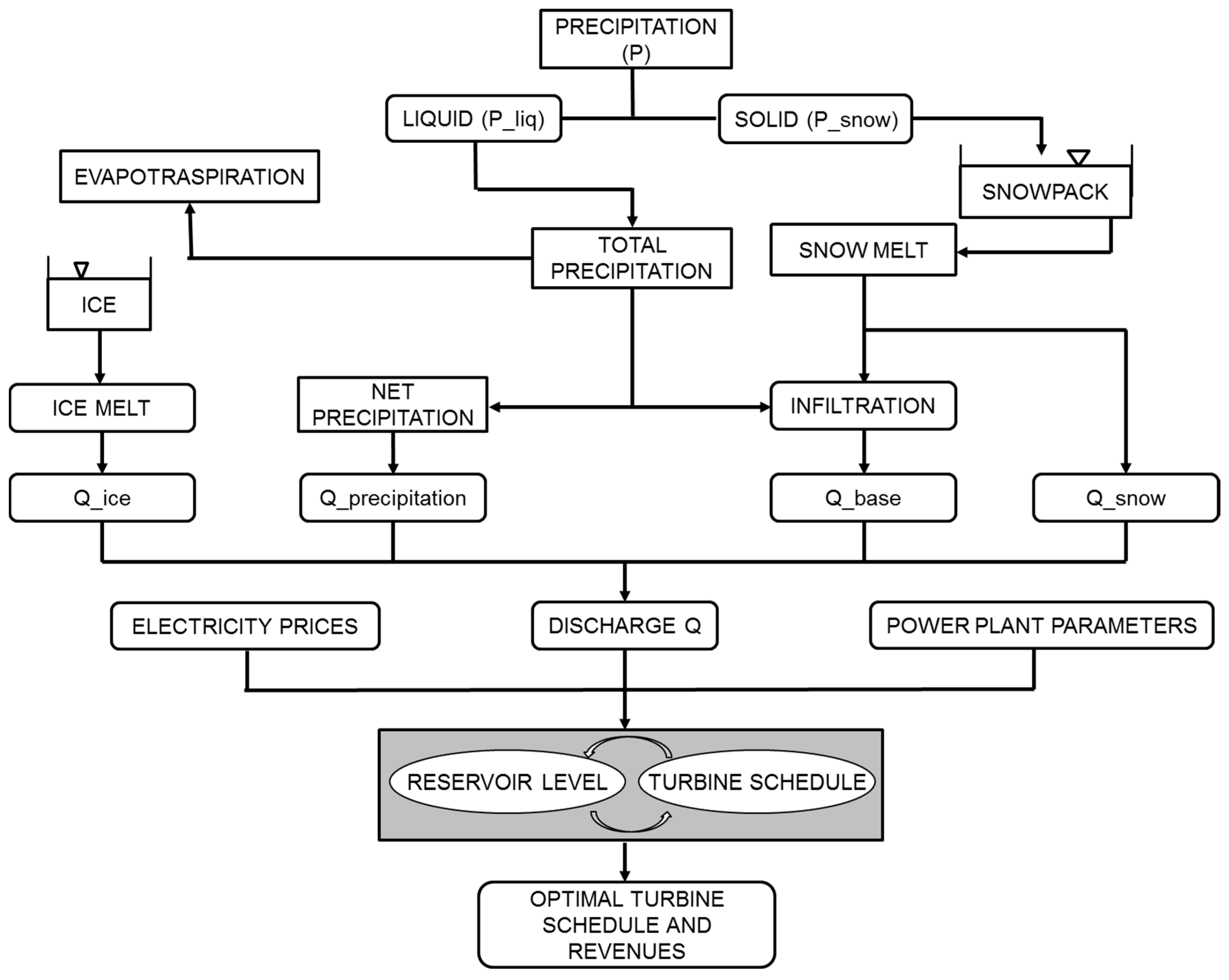
We used a semi-distributed hydrological model following Bongio et al. [25], Patro et al. [18], and Ranzani et al. [59]. The basin was subdivided into independent sub-domain elevation bands with homogeneous geomorphological characteristics. The model simulates the average daily discharge flowing to the closing section, i.e., the Sabbione hydropower plant, from the topographic information, the local precipitation, and temperature data series. The total discharge is calculated as the sum of four distinct contributions: snow melt, glacial melt, rainfall runoff, and base/groundwater flow. The nivometer and the rain gauge approach [85] separate solid from liquid precipitation, while the degree-day model [86,87] treated snow and glacier melt. The mass balance of the glaciers was calculated at yearly scale considering mass-conservation law and neglecting any motion associated. We computed evapotranspiration with a long-term average temperature criterion [88,89], and effective net precipitation and infiltration with the Curve Number method [90]. Finally, a Nash approach computes all the components at the closing section [91]. A schematic representation of the model can be seen in Figure 2.
Rosso [92] formula estimated the Nash parameters for the basin response to liquid precipitation. These are expressed as monomial functions of hortonian ratios RB, RL, RA and the time scale factor LΩ/V.
where LΩ (km) indicates the length of the main stream, V (m/s) the average streamflow velocity of a flood wave in the hydrographic network. From the literature, V assumes values between 2 and 3 m/s, in this work it was assumed equal to 2.5 m/s [92]. Hortonian ratios were evaluated from the quantitative geomorphological description of the hydrographic network, using the Horton–Strahler hierarchical model. The estimation of all the parameters was done using GIS software, to obtain the Horton–Strahler classification for the Sabbione catchment. The results found and the parameters obtained are shown in Table 4.
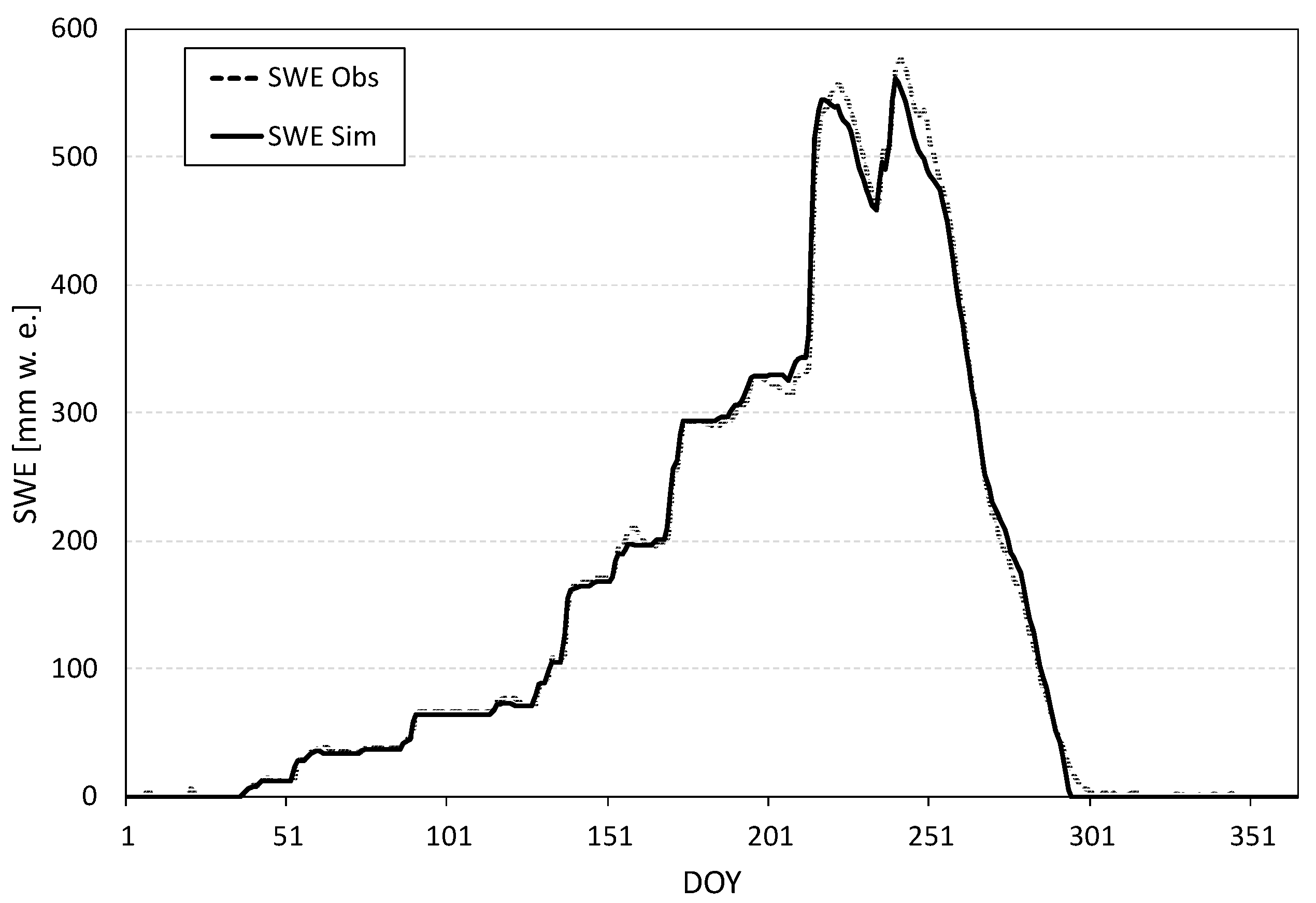
In order to evaluate the maximum and minimum degree day parameters, DDFMAX and DDFMIN respectively, were determined using processing-modelling as reported in Avanzi et al. [93]. We calibrated the model with the meteorological dataset provided by the Regional Agency for Environmental Protection (ARPA Piemonte). The available daily meteorological data include precipitation, temperature, and snow depth from 2000 to 2014 for the Formazza meteorological station located at an altitude of 2453 m.a.s.l. The calibration was done minimizing the Root Mean Square Error (RMSE) (mm w. e.), obtained by comparing simulated and real values of snow water equivalent (SWE) for all the series available.
The values obtained from this phase were DDFMAX = 1.77 mm/d °C and DDFMIN = 0.99 mm/d °C. Figure 3 compares the simulated and observed SWE for the best year of calibration (2001–2002).
Concerning the temperature lapse rate (TLR), it was calibrated comparing the temperatures recorded by some stations at high altitude in Piedmont region with the ones computed with the following formulation:
where Thigher elevation is the temperature observed at the meteorological station located at higher altitude while Tlower elevation is the temperature observed at the lower altitude meteorological station, and dH is the difference in the altitude of the two stations under consideration. Therefore, starting from temperature series recorded by lower altitude stations, TLR was computed minimizing the error between simulated and observed ones. The stations of each pair belong to the same catchment and are available in ARPA Piemonte website (http://www.arpa.piemonte.it/) is as follow:
- Alagna (1347 m.a.s.l.) and Bocchetta delle Pisse (2410 m.a.s.l.);
- Balme (1410 m.a.s.l) and Rifugio Gastaldi (2659 m.a.s.l);
- Macugnaga Pecetto (1360 m.a.s.l) and Rifugio Zamboni (2075 m.a.s.l);
- Noasca (1055 m.a.s.l) and Lago Agnel (2304 m.a.s.l);
- Prerichard (1353 m.a.s.l) and Rochemolles (1965 m.a.s.l).
The calibration obtained a value of TLR equal to 0.53 °C/100 m, consistent with the values found by Rolland [94]. With all this information, the hydrologic budget was computed for the catchment at daily resolution. This hydrological modelling framework has been tested previously for 42 Italian Alpine catchments of which Sabbione was also considered [18]. The model has proven to provide a sufficiently good performance for the scope of this paper with an average RMSE daily and monthly scale as 2.56 and 1.32 m3/s, and average Nash Sutcliffe efficiency (NSE) daily and monthly scales at −0.14 and 0.63. Further information including details of the model and protocol of calibration and validation can be found in Patro et al. [18].
3.3. Future Climate Scenarios
The future discharge inflow at Sabbione reservoir was computed according to the future scenarios following Patro et al. [18]. Nine scenarios consider direct assumptions on future climatic patterns of two variables: temperature and precipitation. These “local” scenarios impose trends in the historical series of the climatic variables. The adoption of this approach stems from the fact that (a) several uncertainties affect Representative Concentration Pathways for mountainous areas [7]; (b) it allows a direct evaluation of the uncertainty with a Monte Carlo technique compared to IPCC-like outputs [59]. Bongio et al. [25] analyzed these nine scenarios with IPCC-like scenario, proving comparable results. Each scenario simulates 100 time series of discharges to obtain a 95% confidence interval for the time horizon of 1 January 2016–31 December 2046. These nine scenarios were subdivided into four major categories based on variation in precipitation and temperature time series:
- Future-like-present scenarios (scenarios 1 and 2): They evaluate the future evolution of the glaciers at present conditions. Temperature and precipitation assume presents patterns, alternatively considering or neglecting the computation of the mass balance of the glaciers in the basin.
- Warmer future scenarios (scenarios 3–5): They evaluate the effects of positive trends in temperatures (+0.03 °C/y, +0.06 °C/y, and +0.09 °C/y) neglecting any modification of the precipitation pattern on the hydrological regime of the basin. These temperature trends are in line with the scientific literature [8,84,95].
- Liquid-precipitation scenario (scenario 6). This extreme scenario assumes liquid-only precipitation and neglects temperature warming.
- The mixed scenarios (scenarios 7–9): These complex scenarios built random series combining liquid-only precipitation and the three above-mentioned trends of temperature.
3.4. The Hydropower Management Model
We simulated the energy generation schedule with the model proposed in Ranzani et al. [59]. It maximizes the objective function provided in Equation (4). It provides the hydropower plant operator revenue at an annual scale and hourly time granularity. It also adds the value of the residual water (RT) to avoid emptying the reservoir at the end of each simulation. Figure 2 shows the general structure of the management model.
where is water density, g is the acceleration of gravity, c is the water flow through the turbines, η is the plant efficiency, Δt is the time multiplier that corresponds to the unity of time considered for the operations (1 h in the present work), T is the time horizon for the optimization (1 year in this case), ht is the hydraulic head, Pt is the electricity day-ahead price, xt is the scheduling multiplier, and RT is the value of the residual volume of water in the reservoir. The latter represents the virtual revenue that would have been generated with the residual water.
The process of management must respect physical constraints linked to the capacity of the reservoir and of the turbines. Therefore, the overall optimization problem can be formulated as:
The objective function relies on the parameter xt, regulating the amount of discharge released through the penstock. It embodies the scheduling of the turbines as it prescribes the amount of water to be turbined per unit of time. Φ is the function of the reservoir’s height-volume (water level-volume) curve. The model outputs energy generation schedule, revenue, and reservoir water volume behavior.
The model considers a local search algorithm, called Threshold Accepting (TA) [96,97,98] to approximate the objective function maximum. This technique explores the search space by affecting the turbine schedule, so that the choice of a particular setting in the model is mainly linked to the fact that it will permit to easily reach the observed income with low computational weight. It is recorded if the value of the objective function is better. The algorithm accepts a degradation in the objective function if lower to a threshold, which reduces progressively in the search. This approach avoids staying stuck in a local optimum, while staying efficient.
In the absence of data of actual power generated, the model was not validated with real data. Therefore, the configuration found in Ranzani et al. [59] was assumed, as the reliability of the model was demonstrated. We only adapted the parameters of the algorithm to fit with the specific constraints of the Sabbione hydropower installation.
3.5. Electricity Price Scenarios
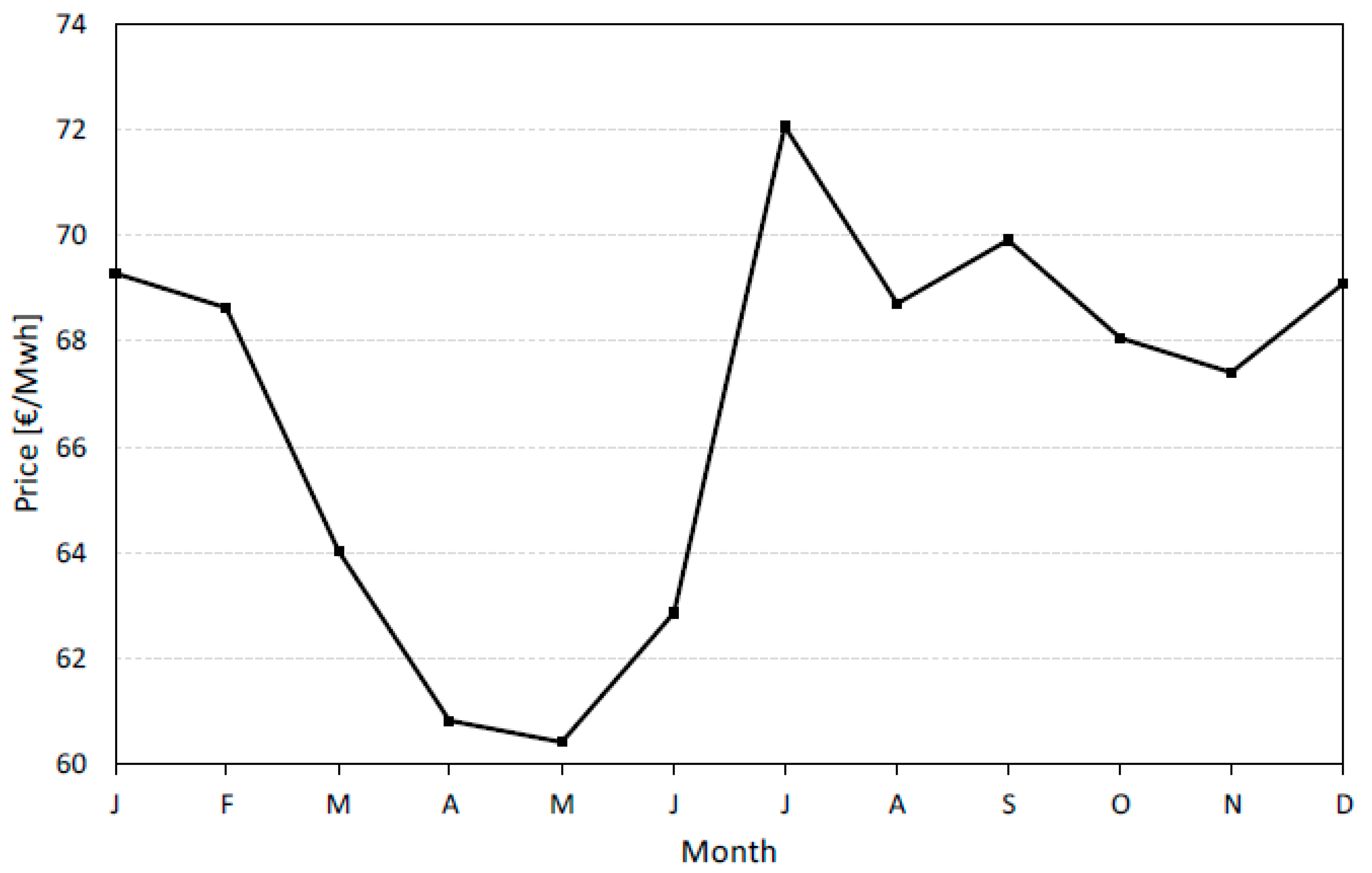
The high uncertainty of long-term electricity price projections determined the necessity of introducing a specific approach. Five electricity price scenarios were taken from Gaudard et al. [26]. Figure 4 shows the average monthly electricity spot price series for Italy (1 January 2005–31 December 2016), taken from Energy Markets Manager (Gestore dei Mercati Energetici, in Italian, see http://www.mercatoelettrico.org/). It shows a double peak, one in winter (heating systems) and the other in summer (cooling system).
We identified the main periodicity in series via a Fourier transform analysis. The first two orders (annual and biannual cycles) put in evidence the historical shape of the periodicity for Italian prices. From this historical periodicity, five scenarios project the evolution of seasonality pattern of electricity spot prices in Italy. Table 5 details the scenarios considered where the annual mean price is constant to focus on the impact of seasonality. The hydropower management model takes into account the streamflow simulated for the future climate and the price trajectories to provide hydropower plant revenue.
4. Results and Discussion
4.1. Climate Change Effects on Glacier and Flow Regimes
We launched the hydrological model from 2016 to 2046. Each climate scenario considered 100 simulations and extracted the 95% confidence interval for each annual discharge. Figure 5 shows the evolution of glacier’s volume over the 30 years.
The rate of glacier retreat is not constant. Until 2030, volumes reduce of almost 50% irrespective of the climate scenario considered. This fast decrease is due to the melting of low altitude glaciers (under 3000 m.a.s.l.), which are more vulnerable to temperature increases [18]. Then, the reduction slows down to reach a new pseudo equilibrium condition. Note that the glacier’s mass balance model neglects the dynamic mobility i.e., the transfer of the upper glacier’s mass to lower one. This could reduce the decrease of volume at lower altitudes and increase the reduction at higher ones [19]. Figure 5 also shows that the glacier’s volume reduces significantly in liquid only precipitation scenarios (6–9) due to the absence of snow that no longer fuels the glacier. The modifications in the hydrological regime play a relevant role in glacier retreat.
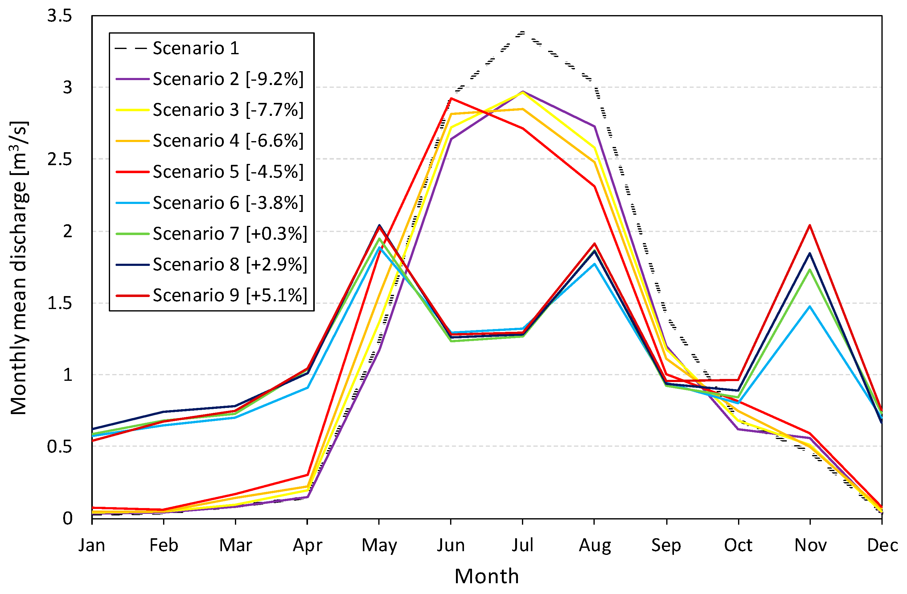
Figure 6 represents the average monthly discharge for the nine climate scenarios in 2030. It also indicates the variation of annual runoff volumes. Presence or absence of glaciers significantly influences the average monthly discharge. The climate scenario 1 (base scenario) neglects the mass balance of glacier, thus observes higher discharge in spring and summer, i.e., when temperature increasing causes the ablation period. In autumn and winter, precipitation governs the discharge. As for climate scenario 2 having meteorological condition as base scenario, the summer peak will decrease due to glacier shrinkage, while the periodicity remains unchanged at 2030. Concerning climate scenarios 3–5, warming affects the hydrological regime with an anticipation of summer peaks due to earlier onset of the ablation of snowpack and glacier. Interestingly, the basin becomes more impulsive and almost equally distributed in the liquid only precipitation scenarios (climate scenarios 6–9). In these scenarios, the curves are almost in phase, differing only in the mean value of discharge.
Figure 5 and Figure 6 combined show the glaciers depletion predominance towards the discharge. The decreasing rate of discharge is higher for climate scenario 2 and progressively reduces as higher trends in temperature (climate scenarios 3–5) are implemented, something that occurs also for climate scenarios 6–9. In fact, the greater temperatures induce a faster regression of the glacier, thus increasing runoff. This compensation would continue until the volume of the glacier is enough to balance the losses due to higher temperatures. The results also reflected those found by Ravazzani et al. [11] on the Toce river basin, which comprises our study area, and differ slightly in the percentages of variation of monthly mean discharge. Ravazzani et al. [11] observed a seasonal shift in monthly discharge with a significant increase in the winter period, while the monthly discharge decreases in summer for the simulation period 2011–2050.
4.2. Climate Change Impact on Reservoir Volumes and Revenue
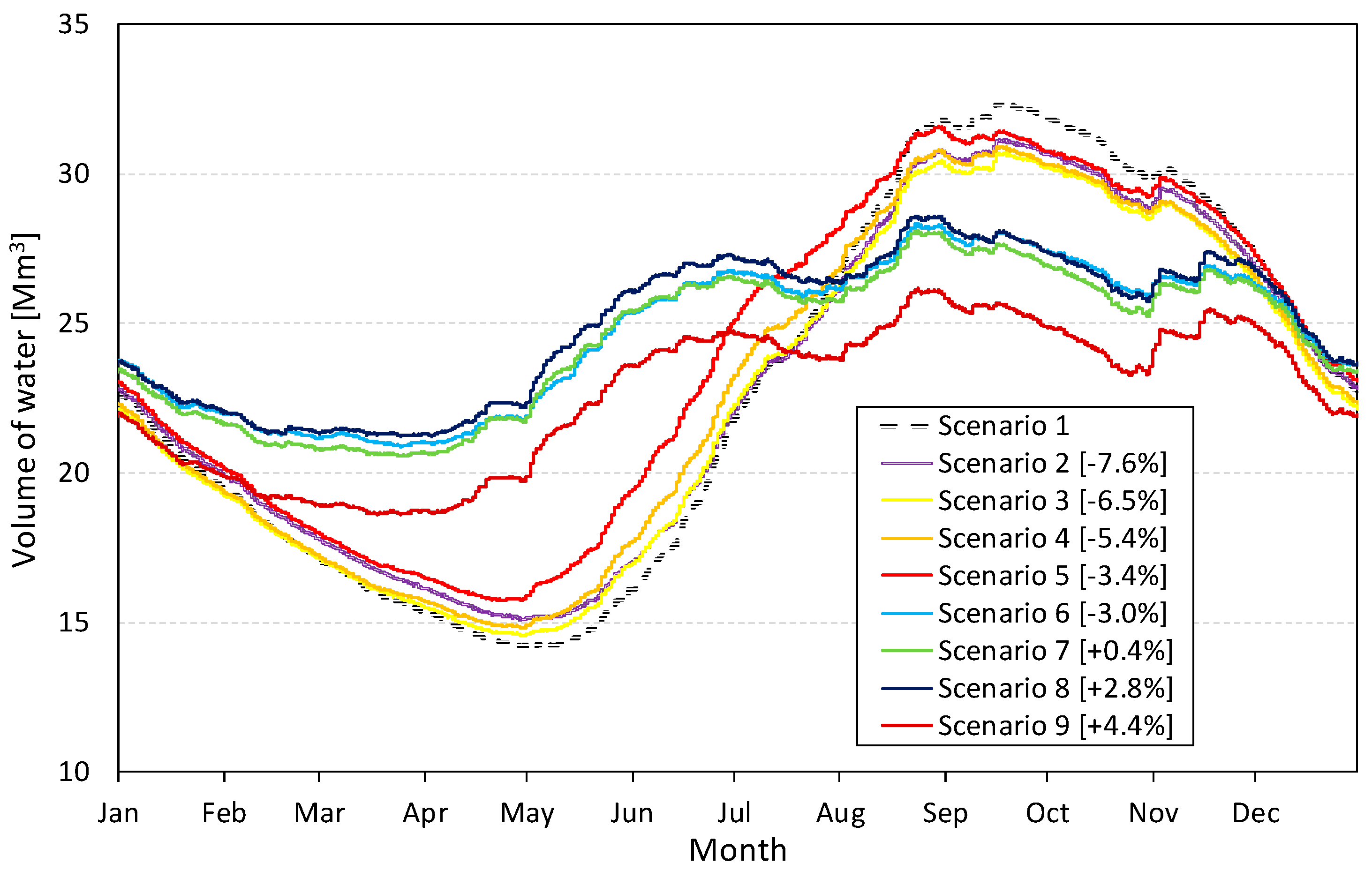
We simulated the hydropower management with the nine climate scenarios discharge series. It provided the reservoir volumes and annual revenue. Figure 7 shows the reservoir’s volume obtained with the historical price setting. The brackets give the relative variations of incomes to base climate scenario 1 in 2030. Please note that the management model tends to keep the upper level of reservoir higher, to exploit the hydraulic head effect. As already observed in Figure 5, the glacier depletion results in a reduction of discharge into the reservoir. However, seasonality matters. In the climate scenarios 1–5, the operator fills the reservoir in spring and summer, when water discharge is high. The warmer the climate is, the earlier the reservoir is filled. The energy is generated when the prices are higher from summer to winter. The reservoir volume largely relies on water seasonality.
In contrast, electricity prices largely determine the reservoir volume shape in the climate scenarios 6–9, where the water seasonality is stable. The reservoir is mostly filled in spring when prices are especially low. The water discharge still affects the reservoir volumes, reflecting similarities found in hydrological regimes. Note that the reservoir used volume is much lower. A smaller dam can be built with low amplitude of water seasonality. Climate change should be considered when designing new projects.
Smart management can mitigate the impact of climate change. Water volumes in Figure 6 vary more than income in Figure 7. The management lowers the negative impact thanks to head effect. In addition, the operator keeps generating electricity during super-peak hours. The only loss in revenue is during low profitability hours. On the other hand, the positive impacts are also tempered in all but scenario 7. Reservoir hydropower can smooth climate change impacts in terms of revenue. This result completely aligns with the finding of Ravazzani et al. [11], where they also concluded that optimal regulation of the Toce river basin hydropower for simulation period 2011–2050, anticipates the date of achieving maximum reservoir volume with drawdown in reservoir volume in August and September to capture the increasing autumn inflows.
4.3. Impact of Electricity Price Scenarios
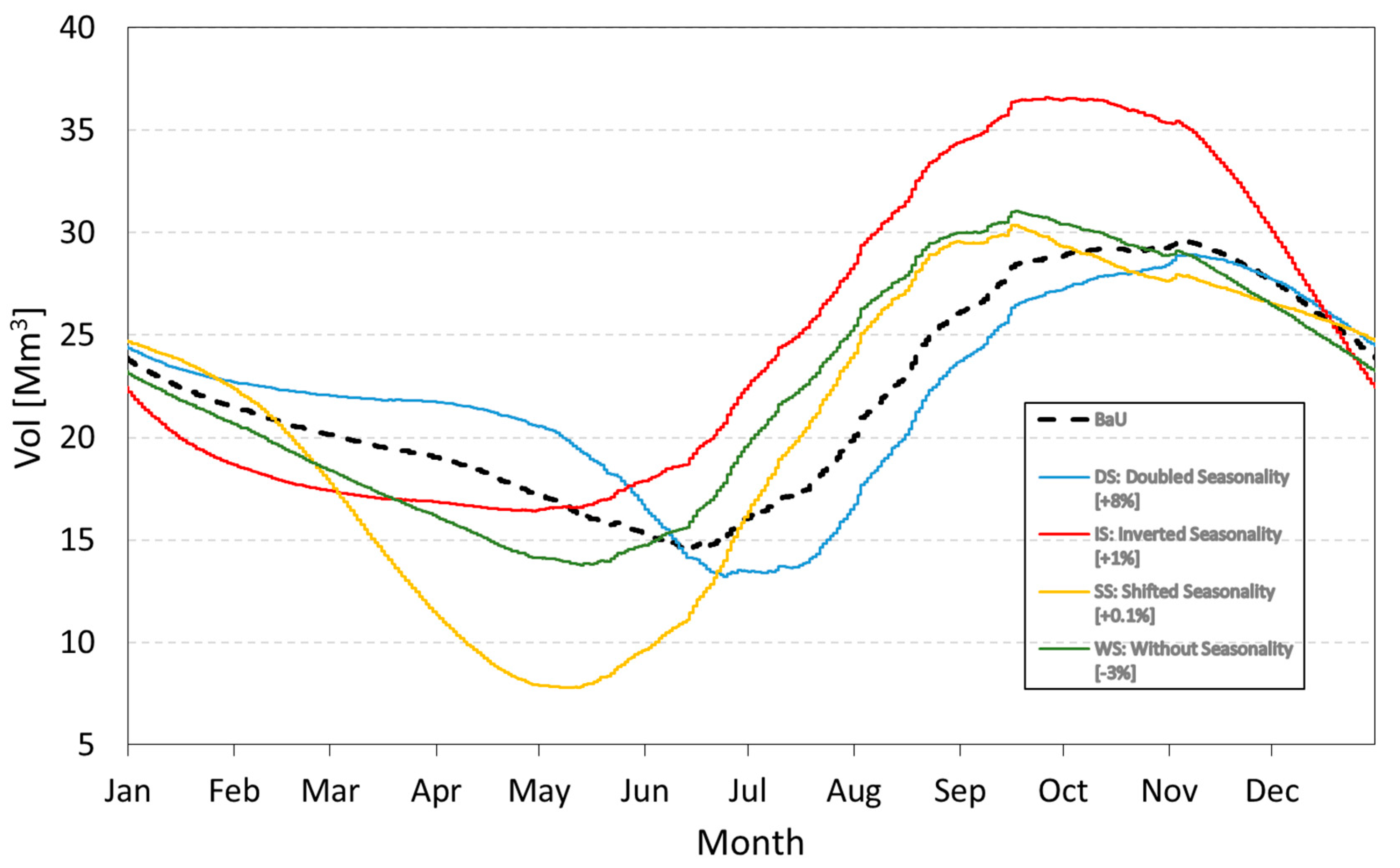
We now analyze the impact of the five different electricity price scenarios. We consider the business-like-present hydrological scenario (climate scenario 1) to focus on the impact of the seasonality of the electric demand. Figure 8 shows the evolution of reservoir’s volumes according to the five price scenarios.
Price seasonality affects the reservoir management. Doubling the amplitude of seasonality (DS) means spring prices are becoming less attractive. The level is flat, has almost no water incomes, and no electricity is being generated. In contrast, summer prices are high, thus the operator generates most of the energy at that period. In the case of inverted seasonality (IS), peak of water income in summer is almost only stored as prices are low. The operator mostly starts generating in winter with a shift of seasonality onward by three months. Finally, without seasonality, the reservoir level is flatter. Energy is generated throughout the year. The reservoir is used to capture the peak hours in the 12 months, as the water mostly intakes in summer. The correlation between water and price seasonality determines reservoir level and optimal design.
The reservoir is large enough to manage a shift of seasonality. IS and SS do not observe a significant variation of revenue (in brackets). In contrast, doubling or removing the amplitude of seasonality affects the revenue. DS and WS keep the mean annual price stable but affect the peak prices. When doubling the amplitude of seasonality, peak prices increase while baseload diminishes. As Sabbione installation can generate during peak price and store during baseload, its revenue significantly increases. Without seasonality, prices are stable over the year and peak prices are smoothed, thus the revenue decreases.
4.4. Impact of Mixed Scenarios
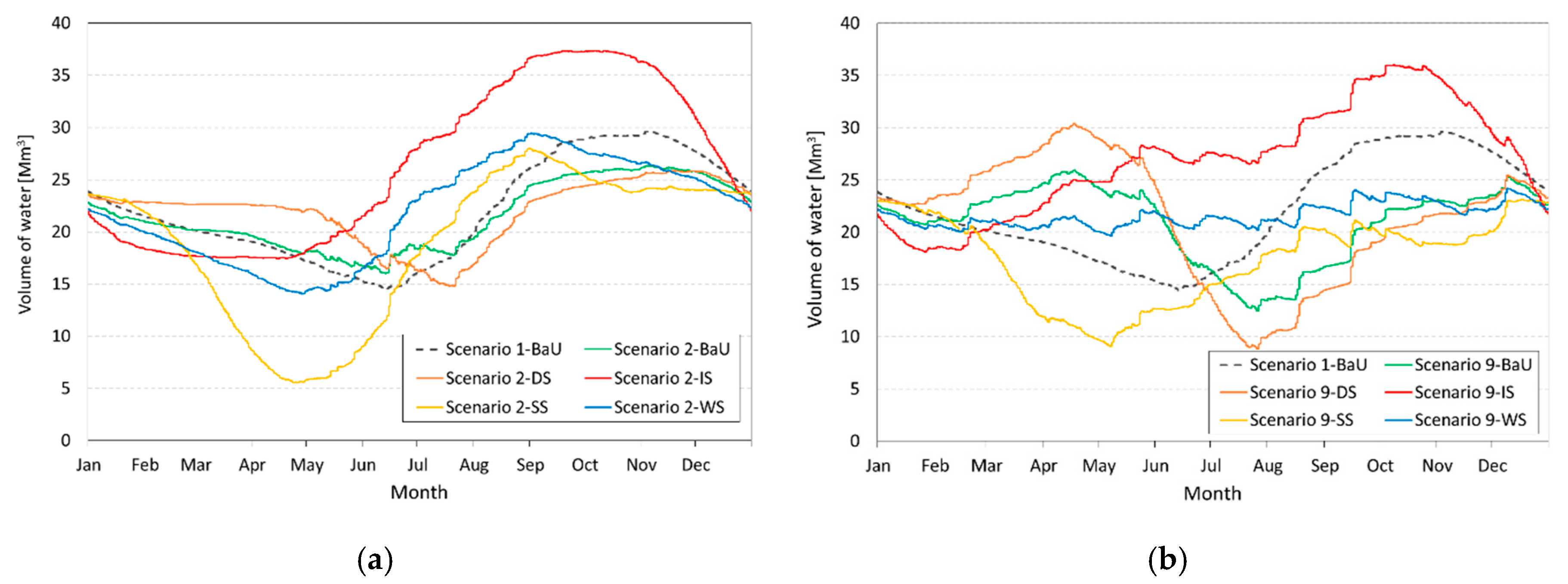
We now combine two climate scenarios (2 and 9) with the five price scenarios to compute the normalized incomes with respect to 2015. We selected these climate scenarios because of their significant impact on the reservoir volume and income (seen in Section 4.1). They serve as a general representation for all other climate scenarios. Figure 9 represents the reservoir water volumes obtained from mixed scenarios while Figure 10 outlines the normalized income with respect to the BaU price scenario of climate scenario 1.
It can be seen in Figure 9a and Figure 10a, the mixed scenario 2-BaU, to compensate the effect of temperature increase the maximum emptying of the reservoir is regulated to take the advantage of head effect, and it is also in phase with the reference business as the present baseline scenario in dashed lines. While, the mixed scenario 2-DS has a trend similar to that observed in Section 4.3, less storage in winter to accommodate for electricity generation when prices are higher. In the mixed scenario 2-WS, the hydropower generation is aligned to the incoming discharge, resulting in emptying of reservoir in winter while filling in the summer to maximize the revenue. While, in Figure 9b and Figure 10b, it is clear that due to strong temperature increment we have maximum incoming discharge during summer due to glacier ablation with anticipation of the summer peaks. Moreover, in mixed scenario 9-BaU, since the seasonality of prices remains constant (double peak in winter and summer) and the seasonality of incoming discharge is negligible, filling happens exactly in the intermediate seasons and the emptying takes place right in summer peak to maximize the revenue. For mixed scenario 9-DS, the management model takes the advantage of peak both in price and discharge, and reservoir volumes are also higher compared to other mixed scenarios. It is fascinating to note that for the mixed scenario 9-WS, the management model operates the hydropower plant as a run-of-the-river configuration, immediately utilizing the incoming discharge for electricity generation, since prices have no seasonality. Figure 10 highlights the fact that change in one scenario (either climate or price) has a limited impact on the management of the reservoir, while combining two scenarios (climate + price), the situation starts to become complex. It therefore highlights that hydropower should be considered with the nexus perspective.
4.5. What If the Reservoir Configuration Becomes a Run of River Model?
A run-of-river power plant design allows grasping the mitigation benefit of a reservoir. Energy generation only depends on the seasonality of inflows, as the operator cannot delay water usage to peak price periods. We simulated this configuration assuming that hydrological runoff is immediately used or released if higher than the turbine capacity. If QF represents the incoming discharge from the river basin and QP the maximum possible discharge through the penstocks, discharge Qt considered for power production is characterized as follows:
if QF > QP, Qt = QP,
if QF < QP, Qt = QF.
if QF < QP, Qt = QF.
We assumed the maximum water head with the reservoir, otherwise it would affect the turbine capacity. It can be viewed as a limit condition to which sedimentation has filled the dam reservoir. Climate change and its impact on glaciers retreat may exacerbate the sedimentation phenomenon [99]. For instance, Ceppo Morelli dam in Italy had an reservoir volume of 0.5 Mm3, reduced to zero nowadays [25,100]. It runs as a run-of-river hydropower plant. Table 6 shows a decrease in the incomes for a RoR configuration compared to the reservoir one, because of a non-optimal management of the production in all climate scenarios. It represents a difference of around −2% for climate scenarios 2–5 and around −4% in the other climate scenarios. The shape of historical electricity prices (Figure 4) obviously impacts the variation. The reduction of discharge in summer (where the prices are higher) and an anticipation of the ablation season in spring (when the prices are lower), have an impact on revenues. The hydrological regime tends to shift and go out of phase with prices. It can be concluded that a run of river power plant revenue is dependent not only on the amount of water income, but also on the behavior of prices. Indeed, considering a different electricity market, e.g., the Swiss one, the effects can be different [59]. Anyway, it proves the mitigation benefits of the reservoir.
Table 7 compares the income variation in Sabbione and of the Ceppo Morelli modelled in Gaudard et al. [26], both with RoR configuration and the five electricity price scenarios. Our RoR configuration results are aligned with those obtained by [26]. The increase and decrease of income are comparable. In contrast, the configurations of Sabbione outline substantial differences. The results are aligned with DS prices, but not with the three remaining price scenarios. RoR configuration is highly sensitive to any changes in the correlation (or non-correlation) between the availability of resources (discharge) and the demand (electricity prices) due to the impracticality to manage the water [26]. Even the DS price scenario observes a higher income increasing with a reservoir than RoR configuration. Reservoir permits not only to compensate future temporal shifting in the electricity price series, minimizing the losses, but also to increase revenues in case future climate scenarios are led to this effect.
5. Conclusions
After a review of the existing literature on the future of Italian hydropower, this study assessed a case study in a multi-driver and multi-model framework, both with presence and absence of storage capacity. The hydrological model utilized nine climate scenarios implementing increasing trends in temperature and modification in the pattern of precipitation, to depict future evolutions of glacier and consequent discharge. Whereas, the management model optimized the energy generation according to five electricity prices scenarios focusing on the modification of seasonality. We considered a horizon of 30 years (2016–2046), assuming 2030 as the reference year for all the scenarios.
The rate of glacier depletion accelerates up to 2030, indicating the importance of glacier retreat in water-energy nexus framework of hydropower. At 2030, climate changes are expected to change seasonality of inflows, with an anticipation of spring peaks due to earlier beginning of snow and glacier ablation. Annual water volumes reduce despite glacier depletion, with values ranging from −9.2% to −4.5% for climate scenarios implementing temperature trends. However, an adequate management can mitigate these losses by optimizing the hydraulic head and the scheduling of turbines. For these scenarios the reduction of revenues is of −7.6% and −3.4%. If changes in price seasonality will modify the operation of the reservoir hydropower plant, only the amplitudes are expected to affect revenues. A temporal shift is ineffective, as the peak prices remain stable.
Run-of-river power plants are highly sensitive to changes in discharge and prices. The absence of a storage capacity cannot mitigate evolution. The comparison between reservoir and RoR configuration outlined the higher robustness of the former to face changes in discharge, as the annual losses of income are 40% lower. These confirm the importance of a storage capacity in compensating the losses and increasing the revenues in most favorable scenarios.
The results of this study are site specific, but some conclusions are general since the results are sufficiently detailed for decision-making and allow us to formulate recommendations for future hydropower investments, especially by connecting these results with the electricity market. The case study represents a good benchmark for researchers and dam managers, since the climate and price scenarios implemented are simple, and suitable for both short-term and long-term climate projections, especially for glacier and/or snow fed catchments. In particular, the liquid only precipitation scenario is extreme but suitable for far-future analysis.
There is still room for further improvements in the water-energy nexus modelling of hydropower. One should consider glacier evolution according to albedo and solar radiation, possible alternative electricity markets such as balancing and ancillary services, combined analysis of hydropower with future climate change perspective of other renewable sources, among others. Hydroelectricity represents an interesting asset in deploying a sustainable energy mix. However, existing installations should be designed in order to limit social and environmental impacts. Therefore, there is greater need to study with a multidisciplinary approach for recognizing the various factors influencing hydropower in the long run.
Author Contributions
Conceptualization, C.D.M.; Methodology, L.G., E.R.P.; Software, A.R., M.B., E.R.P., and L.G.; Validation, E.R.P. and L.G.; Formal Analysis, E.R.P., A.R. and M.B.; Investigation, A.R., M.B. and E.R.P.; Writing—Original Draft Preparation, E.R.P., A.R. and M.B.; Writing—Review and Editing, E.R.P., L.G. and C.D.M.; Visualization, E.R.P.; Supervision, L.G. and C.D.M.
Funding
This research received no external funding.
Acknowledgments
Authors would like to thank ENEL, the company that manages the reservoir, for providing data.
Conflicts of Interest
The authors declare no conflict of interest.
References
- International Renewable Energy Agency (IRENA). Global Energy Transformation: A Roadmap to 2050; IRENA: New York, NY, USA, 2018. [Google Scholar]
- IEA. WEO-2015 Special Report: Energy and Climate Change; IEA: Paris, France, 2015. [Google Scholar]
- Gebretsadik, Y.; Fant, C.; Strzepek, K.; Arndt, C. Optimized reservoir operation model of regional wind and hydro power integration case study: Zambezi basin and South Africa. Appl. Energy 2016, 161. [Google Scholar] [CrossRef]
- Hirth, L. The benefits of flexibility: The value of wind energy with hydropower. Appl. Energy 2016, 181. [Google Scholar] [CrossRef]
- Li, F.F.; Qiu, J. Multi-objective optimization for integrated hydro-photovoltaic power system. Appl. Energy 2016, 167, 377–384. [Google Scholar] [CrossRef]
- Rose, A.; Stoner, R.; Pérez-Arriaga, I. Prospects for grid-connected solar PV in Kenya: A systems approach. Appl. Energy 2016, 161, 583–590. [Google Scholar] [CrossRef] [Green Version]
- Schaefli, B. Projecting hydropower production under future climates: A guide for decision-makers and modelers to interpret and design climate change impact assessments. Wiley Interdiscip. Rev. Water 2015, 2, 271–289. [Google Scholar] [CrossRef]
- Stocker, T.F.; Qin, D.; Plattner, G.K.; Tignor, M.; Allen, S.K.; Boschung, J.; Nauels, A.; Xia, Y.; Bex, V.; Midgley, P.M. Climate Change 2013: The Physical Science Basis; IPCC: Cambridge, UK; New York, NY, USA, 2013. [Google Scholar]
- Blackshear, B.; Crocker, T.; Drucker, E.; Filoon, J. Hydropower Vulnerability and Climate Change—A Framework for Modeling the Future of Global Hydroelectric Resources; Middlebury College Environmental Studies Senior Seminar: Middlebury, VT, USA, 2011; 82p. [Google Scholar]
- Rothstein, B.; Schroedter-Homscheidt, M.; Häfner, C.; Bernhardt, S.; Mimler, S. Impacts of Climate Change on the Electricity Sector and Possible Adaptation Measures BT—Economics and Management of Climate Change: Risks, Mitigation and Adaptation; Hansjürgens, B., Antes, R., Eds.; Springer: New York, NY, USA, 2008; pp. 231–241. ISBN 978-0-387-77353-7. [Google Scholar]
- Ravazzani, G.; Dalla Valle, F.; Gaudard, L.; Mendlik, T.; Gobiet, A.; Mancini, M. Assessing Climate Impacts on Hydropower Production: The Case of the Toce River Basin. Climate 2016, 4, 16. [Google Scholar] [CrossRef]
- Laternser, M.; Schneebeli, M. Long-term snow climate trends of the Swiss Alps (1931-99). Int. J. Climatol. 2003, 23, 733–750. [Google Scholar] [CrossRef]
- Beniston, M.; Farinotti, D.; Stoffel, M.; Andreassen, L.M.; Coppola, E.; Eckert, N.; Fantini, A.; Giacona, F.; Hauck, C.; Huss, M.; et al. The European mountain cryosphere: A review of its current state, trends, and future challenges. Cryosphere 2018, 12, 759–794. [Google Scholar] [CrossRef]
- Wagner, T.; Themeßl, M.; Schüppel, A.; Gobiet, A.; Stigler, H.; Birk, S. Impacts of climate change on stream flow and hydro power generation in the Alpine region. Environ. Earth Sci. 2017, 76. [Google Scholar] [CrossRef]
- Hughes, M.G.; Robinson, D.A. Historical snow cover variability in the great plains region of the USA: 1910 through to 1993. Int. J. Climatol. 1996, 16, 1005–1018. [Google Scholar] [CrossRef]
- Brown, R.D.; Goodison, B.E. Interannual variability in reconstructed Canadian snow cover, 1915-1992. J. Clim. 1996, 9, 1299–1318. [Google Scholar] [CrossRef]
- Frei, A.; Robinson, D.A. Northern Hemisphere snow extent: Regional variability 1972-1994. Int. J. Climatol. 1999, 19, 1535–1560. [Google Scholar] [CrossRef]
- Patro, E.R.; De Michele, C.; Avanzi, F. Future perspectives of run-of-the-river hydropower and the impact of glaciers’ shrinkage: The case of Italian Alps. Appl. Energy 2018, 231, 699–713. [Google Scholar] [CrossRef]
- Huss, M.; Jouvet, G.; Farinotti, D.; Bauder, A. Future high-mountain hydrology: A new parameterization of glacier retreat. Hydrol. Earth Syst. Sci. 2010, 14, 815–829. [Google Scholar] [CrossRef]
- Schaefli, B.; Manso, P.; Fischer, M.; Huss, M.; Farinotti, D. The role of glacier retreat for Swiss hydropower production. Renew. Energy 2019, 132, 615–627. [Google Scholar] [CrossRef]
- Cat Berro, D.; Acordon, V.; Di Napoli, G. Cambiamenti Climatici Sulla Montagna Piemontese; Società Meteorologica Subalpina: Bussoleno, Italy, 2008; 142p. [Google Scholar]
- Cannone, N.; Diolaiuti, G.; Guglielmin, M.; Smiraglia, C. Accelerating climate change impacts on alpine glacier forefield ecosystems in the European Alps. Ecol. Appl. 2008, 18, 637–648. [Google Scholar] [CrossRef] [PubMed]
- Diolaiuti, G.A.; Maragno, D.; D’Agata, C.; Smiraglia, C.; Bocchiola, D. Glacier retreat and climate change: Documenting the last 50 years of Alpine glacier history from area and geometry changes of Dosdè Piazzi glaciers (Lombardy Alps, Italy). Prog. Phys. Geogr. 2011, 35, 161–182. [Google Scholar] [CrossRef]
- Beniston, M. Impacts of climatic change on water and associated economic activities in the Swiss Alps. J. Hydrol. 2012, 412–413, 291–296. [Google Scholar] [CrossRef]
- Bongio, M.; Avanzi, F.; De Michele, C. Hydroelectric power generation in an Alpine basin: Future water-energy scenarios in a run-of-the-river plant. Adv. Water Resour. 2016, 94, 318–331. [Google Scholar] [CrossRef]
- Gaudard, L.; Avanzi, F.; De Michele, C. Seasonal aspects of the energy-water nexus: The case of a run-of-the-river hydropower plant. Appl. Energy 2018, 210, 604–612. [Google Scholar] [CrossRef]
- Etter, S.; Addor, N.; Huss, M.; Finger, D. Climate change impacts on future snow, ice and rain runoff in a Swiss mountain catchment using multi-dataset calibration. J. Hydrol. Reg. Stud. 2017, 13, 222–239. [Google Scholar] [CrossRef]
- Finger, D.; Heinrich, G.; Gobiet, A.; Bauder, A. Projections of future water resources and their uncertainty in a glacierized catchment in the Swiss Alps and the subsequent effects on hydropower production during the 21st century. Water Resour. Res. 2012, 48. [Google Scholar] [CrossRef] [Green Version]
- Ceppi, A.; Ravazzani, G.; Salandin, A.; Rabuffetti, D.; Montani, A.; Borgonovo, E.; Mancini, M. Effects of temperature on flood forecasting: Analysis of an operative case study in Alpine basins. Nat. Hazards Earth Syst. Sci. 2013, 13, 1051–1062. [Google Scholar] [CrossRef]
- Montaldo, N.; Ravazzani, G.; Mancini, M. On the prediction of the Toce alpine basin floods with distributed hydrologic models. Hydrol. Process. 2007. [Google Scholar] [CrossRef]
- Ravazzani, G.; Barbero, S.; Salandin, A.; Senatore, A.; Mancini, M. An integrated Hydrological Model for Assessing Climate Change Impacts on Water Resources of the Upper Po River Basin. Water Resour. Manag. 2014. [Google Scholar] [CrossRef]
- Ravazzani, G.; Ghilardi, M.; Mendlik, T.; Gobiet, A.; Corbari, C.; Mancini, M. Investigation of climate change impact on water resources for an alpine basin in northern Italy: Implications for evapotranspiration modeling complexity. PLoS ONE 2014. [Google Scholar] [CrossRef] [PubMed]
- Gaudard, L.; Romerio, F. Reprint of “The future of hydropower in Europe: Interconnecting climate, markets and policies”. Environ. Sci. Policy 2014, 43, 5–14. [Google Scholar] [CrossRef]
- Apadula, F.; Bassini, A.; Elli, A.; Scapin, S. Relationships between meteorological variables and monthly electricity demand. Appl. Energy 2012, 98, 346–356. [Google Scholar] [CrossRef]
- Bartos, M.; Chester, M.; Johnson, N.; Gorman, B.; Eisenberg, D.; Linkov, I.; Bates, M. Impacts of rising air temperatures on electric transmission ampacity and peak electricity load in the United States. Environ. Res. Lett. 2016, 11. [Google Scholar] [CrossRef]
- Kern, F.; Smith, A. Restructuring energy systems for sustainability? Energy transition policy in the Netherlands. Energy Policy 2008, 36, 4093–4103. [Google Scholar] [CrossRef]
- Scott, C.A.; Pierce, S.A.; Pasqualetti, M.J.; Jones, A.L.; Montz, B.E.; Hoover, J.H. Policy and institutional dimensions of the water-energy nexus. Energy Policy 2011, 39, 6622–6630. [Google Scholar] [CrossRef]
- Golombek, R.; Kittelsen, S.A.C.; Haddeland, I. Climate change: Impacts on electricity markets in Western Europe. Clim. Chang. 2012, 113, 357–370. [Google Scholar] [CrossRef] [PubMed]
- Ahmed, T.; Muttaqi, K.M.; Agalgaonkar, A.P. Climate change impacts on electricity demand in the State of New South Wales, Australia. Appl. Energy 2012, 98, 376–383. [Google Scholar] [CrossRef]
- Christenson, M.; Manz, H.; Gyalistras, D. Climate warming impact on degree-days and building energy demand in Switzerland. Energy Convers. Manag. 2006, 47, 671–686. [Google Scholar] [CrossRef]
- Schaefli, B.; Hingray, B.; Musy, A. Climate change and hydropower production in the Swiss Alps: Quantification of potential impacts and related modelling uncertainties. Hydrol. Earth Syst. Sci. 2007, 11, 1191–1205. [Google Scholar] [CrossRef]
- Guegan, M.; Madani, K.; Uvo, C.B. Climate Change Effects on the High Elevation Hydropower System with Consideration of Warming Impacts on Electricity Demand and Pricing; California Energy Commission: Sacramento, CA, USA, 2012.
- Malik, R.P.S. Water-energy nexus in resource-poor economies: The Indian experience. Int. J. Water Resour. Dev. 2002. [Google Scholar] [CrossRef]
- Siddiqi, A.; Anadon, L.D. The water-energy nexus in Middle East and North Africa. Energy Policy 2011, 39, 4529–4540. [Google Scholar] [CrossRef]
- Madani, K.; Guégan, M.; Uvo, C.B. Climate change impacts on high-elevation hydroelectricity in California. J. Hydrol. 2014, 510, 153–163. [Google Scholar] [CrossRef]
- Gaudard, L.; Gilli, M.; Romerio, F. Climate Change Impacts on Hydropower Management. Water Resour. Manag. 2013, 27, 5143–5156. [Google Scholar] [CrossRef] [Green Version]
- Maran, S.; Volonterio, M.; Gaudard, L. Climate change impacts on hydropower in an alpine catchment. Environ. Sci. Policy 2014, 43, 15–25. [Google Scholar] [CrossRef]
- International Hydropower Association. Hydropower Status Report (2018); International Hydropower Association: London, UK, 2018; Available online: https://www.hydropower.org/sites/default/files/publications-docs/2018_hydropower_status_report_0.pdf (accessed on 24 June 2019).
- Agrillo, A.; Dal Verme, M.; Liberatore, P.; Lipari, D.; Maio, V.; Surace, V.; Benedetti, L. Rapporto Statistico 2017 Fonti Rinnovabili; Gestore dei Servizi Energetici S.p.A: Rome, Italy, 2018. [Google Scholar]
- Terna. Dati Statistici Sull’energia Elettrica in Italia. Available online: https://www.terna.it/it-it/%0Asistemaelettrico/statisticheeprevisioni/datistatistici.aspx (accessed on 24 June 2019).
- Miglietta, P.P.; Morrone, D.; De Leo, F. The water footprint assessment of electricity production: An overview of the economic-water-energy nexus in Italy. Sustainability 2018, 10, 228. [Google Scholar] [CrossRef]
- Unione Petrolifera. Available online: http://www.unionepetrolifera.it/?page_id=6419 (accessed on 21 June 2019).
- Italy’s National Energy Strategy. 2017. Available online: https://www.mise.gov.it/images/stories/documenti/BROCHURE_ENG_SEN.PDF (accessed on 24 June 2019).
- Proposta Di Piano Nazionale Integrato Per L’energia E Il Clima. 2018. Available online: https://www.mise.gov.it/images/stories/documenti/Proposta_di_Piano_Nazionale_Integrato_per_Energia_e_il_Clima_Italiano.pdf (accessed on 26 Jun 2019).
- International Energy Agency (IEA). Energy Policies of IEA Countries: Italy 2016 Review; IEA: Paris, France, 2016. [Google Scholar]
- Gaudard, L.; Madani, K. Energy storage race: Has the monopoly of pumped-storage in Europe come to an end? Energy Policy 2019. [Google Scholar] [CrossRef]
- Autorità Di Regolazione Per Energia Reti E Ambiente (ARERA)—Relazioni Annuali Sullo Stato Dei Servizi e Sull’attività Svolta. Presidenza del Consiglio dei Ministri, Dipartimento per L’informazione e L’editoria. Available online: https://www.arera.it/it/index.htm (accessed on 26 June 2019).
- Barnett, T.P.; Adam, J.C.; Lettenmaier, D.P. Potential impacts of a warming climate on water availability in snow-dominated regions. Nature 2005, 438, 303–309. [Google Scholar] [CrossRef] [PubMed]
- Ranzani, A.; Bonato, M.; Patro, E.; Gaudard, L.; De Michele, C. Hydropower Future: Between Climate Change, Renewable Deployment, Carbon and Fuel Prices. Water 2018, 10, 1197. [Google Scholar] [CrossRef]
- Farinotti, D.; Usselmann, S.; Huss, M.; Bauder, A.; Funk, M. Runoff evolution in the Swiss Alps: Projections for selected high-alpine catchments based on ENSEMBLES scenarios. Hydrol. Process. 2012, 26, 1909–1924. [Google Scholar] [CrossRef]
- Horton, P.; Schaefli, B.; Mezghani, A.; Hingray, B.; Musy, A. Assessment of climate-change impacts on alpine discharge regimes with climate model uncertainty. Hydrol. Process. 2006, 20, 2091–2109. [Google Scholar] [CrossRef]
- Addor, N.; Rössler, O.; Köplin, N.; Huss, M.; Weingartner, R.; Seibert, J. Robust changes and sources of uncertainty in the projected hydrological regimes of Swiss catchments. Water Resour. Res. 2014, 50, 7541–7562. [Google Scholar] [CrossRef] [Green Version]
- Smiraglia, C.; Azzoni, R.S.; D’agata, C.; Maragno, D.; Fugazza, D.; Diolaiuti, G.A. The evolution of the Italian glaciers from the previous data base to the new Italian inventory. Preliminary considerations and results. Geogr. Fis. Din. Quat. 2015, 38, 79–87. [Google Scholar] [CrossRef]
- Smiraglia, C.; Diolaiuti, G. The New Italian Glacier Inventory; Ev-K2-CNR Publish: Bergamo, Italy, 2015; 400p, ISBN 9788894090802. [Google Scholar]
- Comitato Glaciologico Italiano; Consiglio Nazionale delle Ricerche. Catasto dei Ghiacciai Italiani, Anno Geofisico Internazionale 1957–1958; Elenco generale e bibliografia dei ghiacciai italiani; CGI, CNR; Comitato Glaciologico Italiano: Torino, Italy, 1959; Volume 1, 172p. [Google Scholar]
- Berga, L. The Role of Hydropower in Climate Change Mitigation and Adaptation: A Review. Engineering 2016, 2, 313–318. [Google Scholar] [CrossRef] [Green Version]
- D’Agata, C.; Bocchiola, D.; Soncini, A.; Maragno, D.; Smiraglia, C.; Diolaiuti, G.A. Recent area and volume loss of Alpine glaciers in the Adda River of Italy and their contribution to hydropower production. Cold Reg. Sci. Technol. 2018, 148, 172–184. [Google Scholar] [CrossRef]
- Gaudard, L.; Romerio, F.; Dalla Valle, F.; Gorret, R.; Maran, S.; Ravazzani, G.; Stoffel, M.; Volonterio, M. Climate change impacts on hydropower in the Swiss and Italian Alps. Sci. Total Environ. 2014, 493, 1211–1221. [Google Scholar] [CrossRef] [PubMed]
- Jacob, D. A note to the simulation of the annual and inter-annual variability of the water budget over the Baltic Sea drainage basin. Meteorol. Atmos. Phys. 2001, 77, 61–73. [Google Scholar] [CrossRef]
- Pal, J.S.; Giorgi, F.; Bi, X.; Elguindi, N.; Solmon, F.; Gao, X.; Rauscher, S.A.; Francisco, R.; Zakey, A.; Winter, J.; et al. Regional climate modeling for the developing world: The ICTP RegCM3 and RegCNET. Bull. Am. Meteorol. Soc. 2007. [Google Scholar] [CrossRef]
- Ciarapica, L.; Todini, E. TOPKAPI: A model for the representation of the rainfall-runoff process at different scales. Hydrol. Process. 2002. [Google Scholar] [CrossRef]
- Boscarello, L.; Ravazzani, G.; Rabuffetti, D.; Mancini, M. Integrating glaciers raster-based modelling in large catchments hydrological balance: The Rhone case study. Hydrol. Process. 2014, 28, 496–508. [Google Scholar] [CrossRef]
- Majone, B.; Villa, F.; Deidda, R.; Bellin, A. Impact of climate change and water use policies on hydropower potential in the south-eastern Alpine region. Sci. Total Environ. 2016, 543, 965–980. [Google Scholar] [CrossRef]
- Bellin, A.; Majone, B.; Cainelli, O.; Alberici, D.; Villa, F. A continuous coupled hydrological and water resources management model. Environ. Model. Softw. 2016, 75, 176–192. [Google Scholar] [CrossRef]
- Mereu, S.; Sušnik, J.; Trabucco, A.; Daccache, A.; Vamvakeridou-Lyroudia, L.; Renoldi, S.; Virdis, A.; Savić, D.; Assimacopoulos, D. Operational resilience of reservoirs to climate change, agricultural demand, and tourism: A case study from Sardinia. Sci. Total Environ. 2016, 543, 1028–1038. [Google Scholar] [CrossRef] [Green Version]
- Ranzi, R.; Barontini, S.; Grossi, G.; Faggian, P.; Kouwen, N.; Maran, S. Impact of climate change scenarios on water resources management in the Italian Alps. In Proceedings of the IAHR Congress, Vancouver, BC, Canada, 9–14 August 2009; p. 8. [Google Scholar]
- Aronica, G.T.; Bonaccorso, B. Climate change effects on hydropower potential in the Alcantara River basin in Sicily (Italy). Earth Interact. 2013, 17. [Google Scholar] [CrossRef]
- Bombelli, G.M.; Soncini, A.; Bianchi, A.; Bocchiola, D. Potentially modified hydropower production under climate change in the Italian Alps. Hydrol. Process. 2019. [Google Scholar] [CrossRef]
- Hamududu, B.; Killingtveit, A. Assessing climate change impacts on global hydropower. Energies 2012, 5, 305–322. [Google Scholar] [CrossRef]
- François, B.; Hingray, B.; Borga, M.; Zoccatelli, D.; Brown, C.; Creutin, J.-D. Impact of Climate Change on Combined Solar and Run-of-River Power in Northern Italy. Energies 2018, 11, 290. [Google Scholar] [CrossRef]
- Tobin, I.; Greuell, W.; Jerez, S.; Ludwig, F.; Vautard, R.; van Vliet, M.T.H.; Bréon, F.-M. Vulnerabilities and resilience of European power generation to 1.5 °C, 2 °C and 3 °C warming. Environ. Res. Lett. 2018, 13, 044024. [Google Scholar] [CrossRef]
- Van Vliet, M.T.H.; Vögele, S.; Rübbelke, D. Water constraints on European power supply under climate change: Impacts on electricity prices. Environ. Res. Lett. 2013, 8. [Google Scholar] [CrossRef]
- Lehner, B.; Czisch, G.; Vassolo, S. The impact of global change on the hydropower potential of Europe: A model-based analysis. Energy Policy 2005, 33, 839–855. [Google Scholar] [CrossRef]
- Giaccone, E.; Colombo, N.; Acquaotta, F.; Paro, L.; Fratianni, S. Climate variations in a high altitude alpine basin and their effects on a glacial environment (Italian Western Alps). Atmosfera 2015, 28, 117–128. [Google Scholar] [CrossRef]
- Avanzi, F.; Yamaguchi, S.; Hirashima, H.; De Michele, C. Bulk volumetric liquid water content in a seasonal snowpack: Modeling its dynamics in different climatic conditions. Adv. Water Resour. 2015, 86, 1–13. [Google Scholar] [CrossRef]
- Hock, R. Glacier melt: A review of processes and their modelling. Prog. Phys. Geogr. 2005, 29, 362–391. [Google Scholar] [CrossRef]
- Singh, P. Snow and Glacier Hydrology, 1st ed.; Springer: Dordrecht, The Netherlands, 2011; ISBN 9789048156351. [Google Scholar]
- Thornthwaite, C.W. An Approach toward a Rational Classification of Climate. Geogr. Rev. 1948, 38, 55–94. [Google Scholar] [CrossRef]
- Bartolini, E.; Allamano, P.; Laio, F.; Claps, P. Runoff regime estimation at high-elevation sites: A parsimonious water balance approach. Hydrol. Earth Syst. Sci. 2011, 15, 1661–1673. [Google Scholar] [CrossRef]
- U.S. Department of Agriculture. Mockus Victor Design Hydrographs. In National Engineering Handbook; U.S. Department of Agriculture: Washington, DC, USA, 1972; p. 127. [Google Scholar]
- Nash, J.E. The form of the instantaneous unit hydrograph. Int. Assoc. Hydrol. Sci. 1957, 45, 114–121. [Google Scholar]
- Rosso, R. Nash Model Relation to Horton Order Ratios. Water Resour. Res. 1984, 20, 914–920. [Google Scholar] [CrossRef]
- Avanzi, F.; De Michele, C.; Ghezzi, A.; Jommi, C.; Pepe, M. A processing-modeling routine to use SNOTEL hourly data in snowpack dynamic models. Adv. Water Resour. 2014, 73, 16–29. [Google Scholar] [CrossRef]
- Rolland, C. Spatial and seasonal variations of air temperature lapse rates in alpine regions. J. Clim. 2003, 16, 1032–1046. [Google Scholar] [CrossRef]
- Toreti, A.; Desiato, F. Temperature trend over Italy from 1961 to 2004. Theor. Appl. Climatol. 2008, 91, 51–58. [Google Scholar] [CrossRef]
- Dueck, G.; Scheuer, T. Threshold accepting: A general purpose optimization algorithm appearing superior to simulated annealing. J. Comput. Phys. 1990, 90, 161–175. [Google Scholar] [CrossRef]
- Moscato, P.; Fontanari, J.F. Stochastic versus deterministic update in simulated annealing. Phys. Lett. A 1990, 146, 204–208. [Google Scholar] [CrossRef]
- Winker, P. Optimization Heuristics in Econometrics: Application of Threshold Accepting; Wiley: Hoboken, NJ, USA, 2001; ISBN 978-0-471-85631-3. [Google Scholar]
- Peizhen, Z.; Molnar, P.; Downs, W.R. Increased sedimentation rates and grain sizes 2-4 Myr ago due to the influence of climate change on erosion rates. Nature 2001, 410, 891–897. [Google Scholar] [CrossRef]
- De Michele, C.; Salvadori, G.; Canossi, M.; Petaccia, A.; Rosso, R. Bivariate Statistical Approach to Check Adequacy of Dam Spillway. J. Hydrol. Eng. 2005, 10, 50–57. [Google Scholar] [CrossRef]
Figure 1.
(a) Geographical location of the basin in Piedmont region; (b) digital terrain model (DTM) of the Sabbione catchment.
Figure 1.
(a) Geographical location of the basin in Piedmont region; (b) digital terrain model (DTM) of the Sabbione catchment.

Figure 2.
Schematic representation of the hydrological and hydropower management model used.

Figure 3.
Comparison between snow water equivalent (SWE) simulated and observed for the best year of simulation. Please note that the series is considered in hydrological years (1 October 2001–3 September 2002).
Figure 3.
Comparison between snow water equivalent (SWE) simulated and observed for the best year of simulation. Please note that the series is considered in hydrological years (1 October 2001–3 September 2002).

Figure 4.
Average monthly Italian electricity prices obtained from historical time series 2005–2016.
Figure 4.
Average monthly Italian electricity prices obtained from historical time series 2005–2016.

Figure 5.
Evolution of glacier’s volume in the years of simulation.

Figure 6.
Average monthly discharge obtained with a 95% confidence interval at 2030 for all scenarios. The mean annual volume variation relative to climate scenario 1 is presented in brackets.
Figure 6.
Average monthly discharge obtained with a 95% confidence interval at 2030 for all scenarios. The mean annual volume variation relative to climate scenario 1 is presented in brackets.

Figure 7.
Evolution of the reservoir’s volumes for the nine climate scenarios at 2030.The mean income variation w.r.t to base climate scenario 1 are provided in the brackets, with a 95% confidence interval.
Figure 7.
Evolution of the reservoir’s volumes for the nine climate scenarios at 2030.The mean income variation w.r.t to base climate scenario 1 are provided in the brackets, with a 95% confidence interval.

Figure 8.
Evolution of the reservoir’s volumes at 2030 for all price scenarios with a 95% confidence interval. Bracket values show the variations of income compared to business as usual (BaU).
Figure 8.
Evolution of the reservoir’s volumes at 2030 for all price scenarios with a 95% confidence interval. Bracket values show the variations of income compared to business as usual (BaU).

Figure 9.
Evolution of the reservoir’s volumes with a 95% confidence interval at 2030 for mixed scenarios. (a) Climate scenario 2 with all price scenarios and (b) climate scenario 9 with all price scenarios.
Figure 9.
Evolution of the reservoir’s volumes with a 95% confidence interval at 2030 for mixed scenarios. (a) Climate scenario 2 with all price scenarios and (b) climate scenario 9 with all price scenarios.

Figure 10.
Boxplots of the normalized incomes according to 2015 for the mixed scenarios at 2030 scenarios. (a) Climate scenario 2 with all price scenarios and (b) climate scenario 9 with all price scenarios.
Figure 10.
Boxplots of the normalized incomes according to 2015 for the mixed scenarios at 2030 scenarios. (a) Climate scenario 2 with all price scenarios and (b) climate scenario 9 with all price scenarios.


Table 1.
Number and hydropower plants capacity in the Italian regions (source [49]).
Table 1.
Number and hydropower plants capacity in the Italian regions (source [49]).
| Region | Number of Hydropower Plants | Hydropower Potential (MW) |
|---|---|---|
| Piemonte | 905 | 2738.6 |
| Valle d’Aosta | 173 | 974.9 |
| Lombardia | 652 | 5141.4 |
| Trentino Alto Adige | 811 | 3348.4 |
| Veneto | 393 | 1170.6 |
| Friuli Venezia Giulia | 233 | 520.9 |
| Liguria | 88 | 90.4 |
| Emilia Romagna | 194 | 344.7 |
| Toscana | 212 | 372.9 |
| Umbria | 45 | 529.6 |
| Marche | 181 | 250.5 |
| Lazio | 99 | 410.3 |
| Abruzzo | 71 | 1013.3 |
| Molise | 34 | 87.9 |
| Campania | 58 | 342.4 |
| Puglia | 8 | 3.3 |
| Basilicata | 14 | 133.3 |
| Calabria | 54 | 772.5 |
| Sicilia | 25 | 150.7 |
| Sardegna | 18 | 466.4 |
Table 2.
Methodologies and main results of studies on the impacts of climate change on Italian hydropower.
Table 2.
Methodologies and main results of studies on the impacts of climate change on Italian hydropower.
| Study | Location | Climate Projections/Models | Hydrological Model | Other Associated Models | Input of the Model | Evaluation Period | Simulation and Optimization Approach | Main Results |
| [67] | Adda river basin | - | Glacier evolution runoff model neglecting hydrological losses | Glacier area and volume changes using geographic information system (GIS) and digital terrain model (DTM) | Aerial photos, orthophotos, glacier area records, DTM and digital surface model (DSM) products, precipitation | 1981–2007 | - |
|
| [68] | Val d’Aosta and Toce basin | Two RCMs, the REMO [69] and the RegCM3 [70] model | TOPKAPI [71] and FEST-WB [72] model | Electricity demand scenarios and electricity prices models | Temperature, precipitation and electricity prices | 2001–2050 | Deterministic optimization (SOLARIS and BPMPD solver) for the management of hydropower |
|
| [73] | Noce river basin | Ensemble of four climate models (CM) under the SRES A1B emission scenario | GEOTRANSF model [74] | - | Precipitation, temperature and streamflow | 2040–2070 | Particle Swarming Optimizer (PSO) |
|
| [25] | Anza basin at Ceppo Morelli dam | Deterministic climate scenario (temperature increase and liquid only precipitation) and RCP 4.5 and RCP 8.5 | HyM runoff model | Solid-liquid temperature thresholding | Precipitation, temperature streamflow, snow depth, and glacier inventory | 2015–2050 | - |
|
| [75] | Pedra ’e Othoni reservoir in Sardinia | RCPs 4.5 and 8.5 | STELLA Reservoir storage balance model | Precipitation, temperature, agricultural data, and four socio-economic development scenarios | 2035–2065 | - |
| |
| [18] | Italian Alpine-scale (42 basins) | Deterministic climate scenario (combination of temperature increase and liquid only precipitation) | HyM runoff model | Solid-liquid temperature thresholding | Precipitation, temperature and streamflow | 2016–2065 | - |
|
| [47] | Valle d’Aosta | RCM–REMO (25 × 25 km) | TOPKAPI model and SOLARIS model | Electricity demand model | Precipitation, temperature and energy prices | 2011–2050 | - |
|
| [76] | Oglio river basin and Lys river basin | PCM IPCC-SRES A2-scenario | WATFLOOD hydrological model | - | Precipitation, temperature | 2000–2099 | - |
|
| [77] | Alcantara river basin | HadCM3 with A2 and B2 scenarios | IHACRES model | First-order Markov chain and an autoregressive moving average (ARMA) model | Precipitation, temperature, and streamflow | 2013–2037 | - |
|
| [78] | Adda river basin | ECHAM6, CCSM4, EC-EARTH with RCP 2.6, RCP4 and RCP 8.5 scenarios | Poly-Hydro model | Poly-Power model | Precipitation, temperature, and streamflow | 2006–2100 | Mixed Integer Quadratic Programming |
|
| [11] | Toce Alpine river basin | REMO and RegCM3 | FEST-WB model | Model of the hydropower system for maximizing revenue | Temperature, precipitation, and streamflow | 2001–2050 | - |
|
| [79] | National scale derived from worldwide results | 12 GCM models | GIS based model | GRDC dataset for streamflow | 2050 | - |
| |
| [80] | Catchments of Aurino and Posina | CMIP5 with RCP 8.5 | ICHYMOD model | Energy model | Temperature, precipitation, solar irradiance, and streamflow | 1990–2099 | - |
|
| [81] | National scale derived from European-wide results | Five RCM from EUROCORDEX | VIC hydrological model | - | Temperature and precipitation | 1971–2084 | - |
|
| [82] | National scale derived from European-wide results | GCM with IPCC SRES A2 and B1 scenarios. | VIC hydrological model | - | Temperature, precipitation, and daily river flow | 1971–2060 | - |
|
| [83] | National scale derived from European-wide results | HadCM3 model and the ECHAM4/OPYC3 model | WaterGAP model | - | Temperature, precipitation, GRDC dataset for streamflow, and UCTE data tables for hydropower stations | 2070 | - |
|
| [26] | Anza river basin at Ceppo Morelli dam | Deterministic climate scenario (temperature increase and liquid only precipitation) | HyM runoff model | Solid-liquid temperature thresholdingElectricity price and scenarios | Precipitation, temperature, streamflow, snow depth, glacier inventory, and electricity price | 2015–2065 | - |
|
Table 3.
Main features of the Sabbione catchment and Morasco power plant [18].
Table 3.
Main features of the Sabbione catchment and Morasco power plant [18].
| Sabbione Basin and Morasco Power Plant | |
|---|---|
| Catchment area (km2) | ~16.59 |
| Maximum elevation (m.a.s.l.) | 3358 |
| Minimum elevation (m.a.s.l.) | 2399 |
| Average elevation (m.a.s.l.) | 2740 |
| Glacier coverage (%) | 30 |
| Glacier elevation range (m.a.s.l.) | ~2610–3230 |
| Maximum reservoir elevation (m.a.s.l.) | 2460 |
| Minimum reservoir elevation (m.a.s.l.) | 2412 |
| Reservoir Volume available (Mm3) | 44 |
| Maximum discharge (m3/s) | 10.1 |
| Maximum gross jump (m) | 640 |
| Type of turbine | Pelton |
| Power installed (MW) | 45.6 |
| Average production (GWh/year) | 45.4 |
| Efficiency (-) | 0.725 |
Table 4.
Results from Horton–Strahler classification and estimated Nash parameters.
| Order | N. of Streams | Mean Length Stream (km) | RB | RL | RA | V (m/s) | LΩ (km) | nLIQ | kLIQ (hours) |
|---|---|---|---|---|---|---|---|---|---|
| 1 | 20 | 0.38 | 4.472 | 3.638 | 5.619 | 2.5 | 5.03 | 3.014 | 0.235 |
| 2 | 5 | 0.90 | |||||||
| 3 | 1 | 5.03 |
Table 5.
Price scenarios used in this work.
| Scenario | Code Name | Description |
|---|---|---|
| Business as Usual | BaU | In the future the periodicity will remain the same as the historical seasonality (2005–2016) |
| Doubled Seasonality | DS | Seasonality remains but the amplitude is doubled |
| Without Seasonality | WS | Seasonality is discarded, so the prices stay stable all over the year |
| Inverted Seasonality | IS | The seasonality is shifted by six months |
| Shifted Seasonality | SS | Seasonality is shifted onward by three months. This means that the prices will peak in spring and autumn instead of winter and summer. |
Table 6.
Comparison of the income variation between run-of-the-river (RoR) and reservoir configuration in the case of climate scenarios at 2030 w.r.t. baseline climate scenario 1 over historical Italian electricity prices.
Table 6.
Comparison of the income variation between run-of-the-river (RoR) and reservoir configuration in the case of climate scenarios at 2030 w.r.t. baseline climate scenario 1 over historical Italian electricity prices.
| Scenario | Variation Income (-) | |
|---|---|---|
| Reservoir | Run of River | |
| 1 | − | − |
| 2 | −7.6% | −9.4% |
| 3 | −6.5% | −8.1% |
| 4 | −5.4% | −7.3% |
| 5 | −3.4% | −5.8% |
| 6 | −3.0% | −7.2% |
| 7 | +0.4% | −3.7% |
| 8 | +2.8% | −2.3% |
| 9 | +4.4% | −0.4% |
Table 7.
Comparison of the income variation between RoR and reservoir configuration in the case of different price scenarios for Sabbione and income of RoR obtained by Gaudard et al. [26] for Ceppo Morelli.
Table 7.
Comparison of the income variation between RoR and reservoir configuration in the case of different price scenarios for Sabbione and income of RoR obtained by Gaudard et al. [26] for Ceppo Morelli.
| Scenario | Variation Income (-) | ||
|---|---|---|---|
| Sabbione | Ceppo Morelli [26] | ||
| Reservoir | Run of River | Run of River | |
| BaU | − | − | − |
| DS | +8.0% | +6.3% | +5% |
| IS | +0.8% | −6.6% | −7% |
| SS | +0.5% | −18.3% | −11% |
| WS | −3.0% | −6.2% | −5% |
© 2019 by the authors. Licensee MDPI, Basel, Switzerland. This article is an open access article distributed under the terms and conditions of the Creative Commons Attribution (CC BY) license (http://creativecommons.org/licenses/by/4.0/).
Share and Cite
MDPI and ACS Style
Bonato, M.; Ranzani, A.; Patro, E.R.; Gaudard, L.; De Michele, C. Water-Energy Nexus for an Italian Storage Hydropower Plant under Multiple Drivers. Water 2019, 11, 1838. https://doi.org/10.3390/w11091838
AMA Style
Bonato M, Ranzani A, Patro ER, Gaudard L, De Michele C. Water-Energy Nexus for an Italian Storage Hydropower Plant under Multiple Drivers. Water. 2019; 11(9):1838. https://doi.org/10.3390/w11091838
Chicago/Turabian StyleBonato, Mattia, Alessandro Ranzani, Epari Ritesh Patro, Ludovic Gaudard, and Carlo De Michele. 2019. "Water-Energy Nexus for an Italian Storage Hydropower Plant under Multiple Drivers" Water 11, no. 9: 1838. https://doi.org/10.3390/w11091838
Note that from the first issue of 2016, this journal uses article numbers instead of page numbers. See further details here.