A Comprehensive Modelling Approach to Assess Water Use Efficiencies of Different Irrigation Management Options in Rice Irrigation Districts of Northern Italy

Abstract

European rice production is concentrated in limited areas of a small number of countries. Italy is the largest European producer with over half of the total production grown on an area of 220,000 hectares, predominantly located in northern Italy. The traditional irrigation management (wet seeding and continuous flooding until few weeks before harvest—WFL) requires copious volumes of water. In order to propose effective ‘water-saving’ irrigation alternatives, there is the need to collect site-specific observational data and, at the same time, to develop agro-hydrological models to upscale field/farm experimental data to a spatial scale of interest to support water management decisions and policies. The semi-distributed modelling system developed in this work, composed of three sub-models (agricultural area, groundwater zone, and channel network), allows us to describe water fluxes dynamics in rice areas at the irrigation district scale. Once calibrated for a 1000 ha district located in northern Italy using meteorological, hydrological and land-use data of a recent four-year period (2013–2016), the model was used to provide indications on the effects of different irrigation management options on district irrigation requirements, groundwater levels and irrigation/drainage network efficiency. Four scenarios considering a complete conversion of rice irrigation management over the district were implemented: WFL; DFL—dry seeding and delayed flooding; WDA—alternate wetting and drying; WFL-W—WFL followed by post-harvest winter flooding from 15 November to 15 January. Average results for the period 2013–2016 showed that DFL and WDA would lead to a reduction in summer irrigation needs compared to WFL, but also to a postponement of the peak irrigation month to June, already characterized by a strong water demand from other crops. Finally, summer irrigation consumption for WFL-W would correspond to WFL, suggesting that the considered winter flooding period ended too early to influence summer crop water needs.

1. Introduction

In the Mediterranean basin, rice is grown on a surface of 1,300,000 hectares. Italy is the leading producer of rice in Europe, with over half of the total EU production and a high level of quality, and the second rice producer in the Mediterranean area after Egypt. The most important Italian rice area is the portion of the Po Valley located on the left bank of the Po river and along the river Ticino, straddling the regions of Lombardy and Piedmont in northern Italy (about 213,000 hectares in 2017, 93% of the Italian rice area according to Ente Nazionale Risi). In Italy, as well as throughout the Mediterranean basin, rice is traditionally grown in fields flooded from before sowing to a few weeks before harvest: this technique requires much more water than irrigation techniques adopted for other cereals [1,2].

This area is characterized by many peculiarities: a historical abundance of surface water, an ancient and extensive network of unlined irrigation and drainage channels, a complex geo-morphologic and hydro-geologic structure formed by wide fluvioglacial conoids (Pleistocene) cut by river valley lowlands (Holocene) hosting one of the largest aquifers in Europe. Phreatic water levels vary in space and time, and in some areas, they rise up to the topographic surface as a consequence of the summer flooding of paddies. Soils are generally loam/sandy-loam developed on sandy alluvial sediments, with coarser textures occurring along river valleys and finer granulometries in the older (paleo)soils in the northernmost area. Consequently, soils in many areas are generally moderately permeable, and only the peculiar agricultural practices adopted in rice cultivation (mainly flooding) lead to the formation of a dense and low permeable layer below the ploughed horizon, which strongly influences vertical percolation. Additionally, where paddy areas are not perfectly flat (ancient and recent fluvial terraces), local topography may activate lateral water exchanges. All these peculiar aspects lead to a strong interaction between irrigation and surface groundwater dynamics, activated by the huge percolation fluxes from the rice paddies and the unlined canal networks, by the presence of a very shallow aquifer (often within one meter from the seeding bed during the agricultural season), and to a partial reuse of irrigation water, since water losses from fields and canals are partially recovered for irrigation in the downstream agricultural areas. Finally, multi-functionality and eco-system services are actually provided by irrigation systems in many areas (e.g., landscape quality and profitability, ecosystem biodiversity).

In recent years, changed conditions both environmental (greater probability of dry years and more attention of the public opinion to environmental problems) and economic (reduced price of rice, increased competition among water uses), led to the need to re-discuss rice cropping methods in the Lombardy–Piedmont rice basin, as well as in many other rice areas in the world, with the final purpose of introducing ‘water saving’ irrigation methods and practices.

Traditional rice cropping is known to be very water demanding. Water use efficiency (WUE; i.e., ratio between evapotranspiration and water inputs—rain plus irrigation—computed over the cropping season; [3]) is a well-known indicator of the ‘goodness’ of irrigation management in terms of water saving. It is recognized [1] that WUE depends on the spatial scale to which hydrological processes are observed. On a field scale, water losses due to evaporation, irrigation tailwater, seepage through the bunds and percolation below the root zone can be considered ‘non-beneficial’ losses. On larger scales (e.g., irrigation district, river basin), part of these losses can be recovered since irrigation tailwater, seepage and percolation losses can be partially reused by downstream fields; moreover, shallow groundwater levels (typically found in low-lying fields due to the high percolation rates of uphill paddies) allow the reduction of percolation losses and the activation of capillary rise processes during non-flooding periods. Values of WUE reported in the literature for individual paddies are very variable (much more than for other crops), since they depend on numerous factors, amongst the most important being topographic gradient, groundwater depth, presence of low permeable soil layers, irrigation method and practices. They are found to vary between 15% for flooded paddies characterized by coarse soils and water tables at depths higher than 1.5 m, and 60% for paddies on heavier soils and groundwater at less than 0.5 m from the soil surface [4,5,6,7,8]. It must be noted that most of the studies have been conducted in Asian countries, where puddling (submerged soil tilling) is performed to reduce soil permeability. When considering the Italian rice basin, few studies have been conducted so far to assess the water balance of rice fields. In [9] the authors computed the water balance for six experimental plots located in Vercelli and characterized by two different water management techniques: WFL—traditional wet seeding and continuous flooding, and DFL—dry seeding and delayed flooding, in order to quantify the water saving potential of DFL. Results showed similar WUEs for the two techniques, close to 20% (mean values over two years). In recent studies carried out in Pavia for single flooded paddies, WUEs of 20–25% were measured on average-textured soils (from sandy-loam to loam) and groundwater table from 50 to 100 cm from the soil surface during summertime; very low or irrelevant WUE differences were found between WFL and DFL [2,10,11]. When soils become heavier (from loam to clay-loam), fields are placed in central position within toposequences, and groundwater table is shallower (within 50 cm from the soil surface), WUE may rise to 60%. Finally, for fields at the bottom of paddy toposequences, WUE even higher than 100% may be observed due to lateral fluxes coming from upper fields and very shallow groundwater levels [10,11]. In this last study, the authors demonstrate that when paddies are placed on a slope, field position within the toposequence is more important in determining WUE than the irrigation method adopted. Moreover, very often WUE measured at the field scale when adopting ‘water saving techniques’ are detected in fields surrounded by traditional paddies maintaining hydrological conditions that guarantee greater WUE compared to what would be achieved if large portions of the territory were converted to the same ‘water saving’ irrigation techniques. This is for instance the case of a WUE of 55% measured for an intermittently irrigated rice field surrounded by traditional paddies in [2].

The huge variability in WUEs at the field scale suggests that many factors must be considered even more when computing this indicator at the irrigation district or larger scales. It is demonstrated [1] that WUE depends on the spatial scale considered: thanks to water recoveries, WUEs for wider areas are expected to be higher than average values measured at the single paddy scale. However, few studies in literature focus on this issue and even less adopt a comprehensive approach able to take into account feedback effects due to groundwater dynamics. Examples of WUE assessment at wider scales can be found in [12], where the authors assessed the application efficiency (without considering the rainfall contribution, which is very low due to semi-arid conditions) of an irrigated rice cropped area in Iran at two spatial scales, finding an average increase of WUE of 14% from the field to the regional scale. The authors in [13] coupled a crop model (CERES-Rice) and a Geographical Information System (GIS) in order to extend crop model simulation results for an Indian watershed to a wider spatial scale. Values of WUE found for the whole study area (512 ha) are about 30% and 50% for traditional flooding and aerobic rice, respectively. In a more recent study conducted in northeast China [14], the authors estimated the WUE at seven different spatial scales, ranging from about 300 ha (the total area served by a single branch ditch) to 100,800 ha (the whole irrigation basin) by applying a distributed water balance model which takes into account a share of reused water from ditches and groundwater contribution. The results showed an increase of WUE values from 66% at the field scale to 90% at wider scales. For the wider scales, the total amount of water reused (derived both from groundwater and drainage ditches) is about 40% of the evapotranspiration flux, highlighting the importance of water recoveries in rice crop systems. To the authors’ knowledge, in northern Italy the only attempt to assess the WUE at the irrigation district scale was performed by [2]. In particular, the increase of the index value in the case of a massive conversion of the traditional irrigation method (FLD) to intermittent irrigation (WDA) was evaluated. Even if the irrigation district (500 ha) was not exactly representative of the Lombardy–Piedmont rice area (only 38% of the agricultural surface was cropped with rice; soils were sandy), and the model developed was quite simplified (concentrated model, channel network efficiency not simulated), the results clearly show that the strong interaction between irrigation water and groundwater levels may reduce the ‘water saving potential’ of alternative irrigation techniques, due to the important drawbacks that a widespread modification of irrigation methods could have on global water dynamics when considering a large portion of territory.

The limited number of studies conducted in northern Italy rice agro-ecosystems suggests that in order to propose effective and efficient irrigation alternatives to the traditional flooding, there is the need to continue to acquire site-specific observational data (Italian paddies differ from paddies in Eastern countries due to climate, soil type, soil management, crop management, rice varieties, etc.) and, at the same time, to identify and develop agro-hydrological models to upscale field/farm experimental data to a spatial scale of interest to support water management decisions and policies (irrigation district or broader). Models must be sufficiently detailed to reproduce water fluxes and storages in the current situation, taking into account the complex interaction among the percolation from fields and irrigation network, shallow aquifers and irrigation recoveries occurring in many rice areas. Moreover, they shall be able to forecast, once properly calibrated, the effects of changes in irrigation technologies and practices adopted in the territory on the water resource system.

The objective of this study was to explore water dynamics and water use efficiencies of different irrigation management alternatives in a 1000 ha irrigation district prevalently cropped with rice (about 90% of the agricultural surface) and located in the Lombardy portion (Lomellina) of the main Italian rice basin. A modelling framework consisting of three sub-models (one for the agricultural areas, one for the groundwater zone, and one for the channel network) was developed, calibrated and applied to investigate water use efficiency values in a four-year period characterized by a progressive change in irrigation management conditions. The calibrated model was then applied to explore the water use efficiency of hypothetical scenarios related to the adoption of alternative irrigation management techniques over the district. In particular, the following irrigation management alternatives were considered in the simulation: (a) traditional wet seeding and continuous flooding (WFL); (b) dry seeding and delayed flooding (when rice reaches the 3rd–4th leaf stage, DFL); (c) dry seeding and ‘wetting and drying’ alternate irrigation (WDA); (d) traditional wet seeding and continuous flooding, followed by a winter flooding from 15 November to 15 January (as suggested by a recent measure implemented in the Lombardy RDP 2014–2020, WFL-W).

2. Materials and Methods

2.1. Pilot Study Area

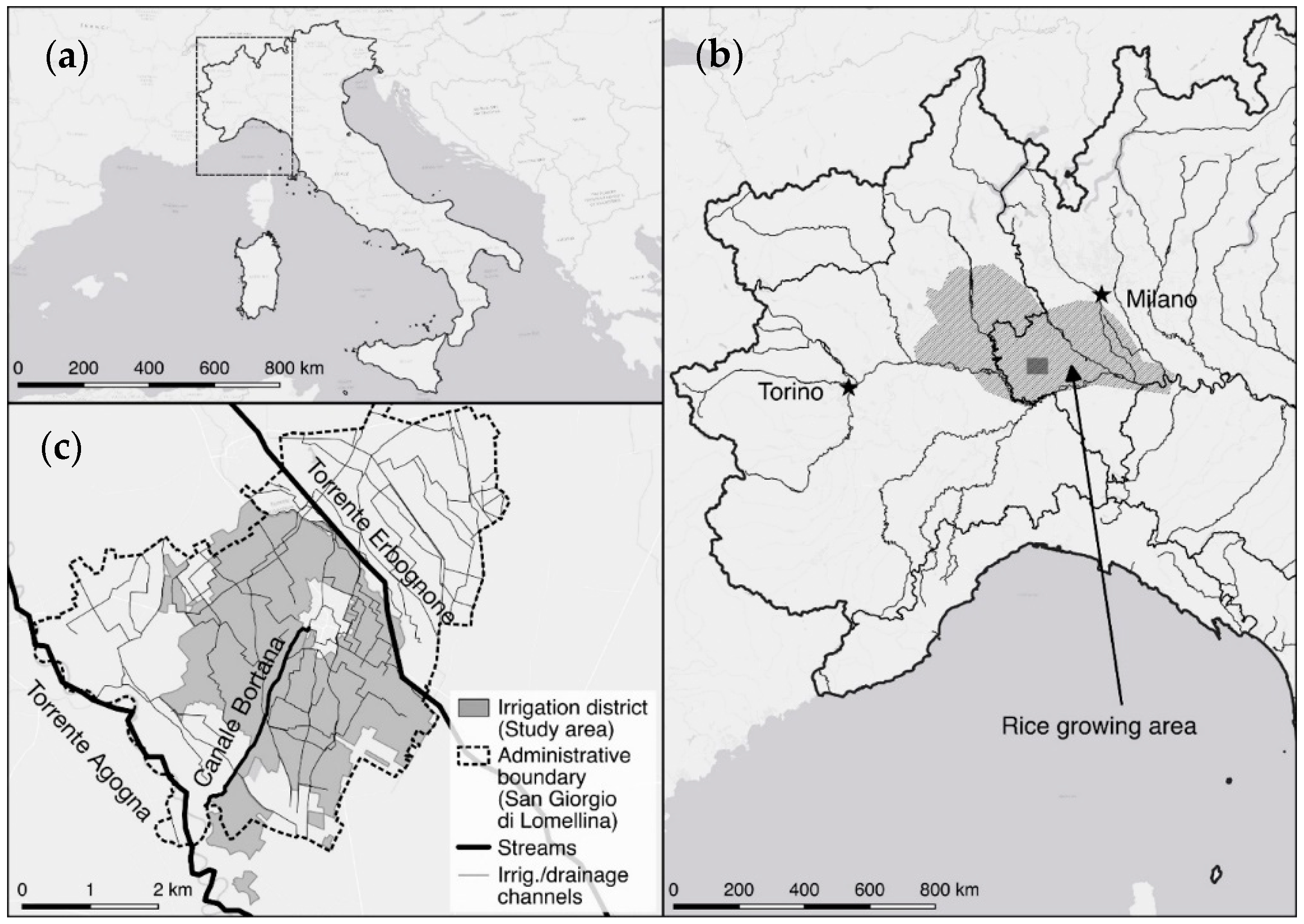
The pilot district is within the administrative boundary of San Giorgio di Lomellina (PV), located about 45 km southwest of the city of Milan and extending over an area of approximately 1000 ha in the Lombardy Plain (Figure 1). The average altitude of the district is 97 m. In the last decade the rice area remained stable at 90% of the agricultural land, while the remaining 10% is mainly cropped with maize and poplar.

From the geomorphological point of view, the district area belongs to the lower part of the alluvial plain originated during the Würm glaciation, started about 100,000–80,000 years ago. The surface is mainly flat except for some sand depositions of fluvial origin resulting few meters higher than the average level of the plain; the uniformity of the plain is also broken by valleys where rivers and streams flow nowadays. Soil textures are typically medium to coarse [15]. The phreatic groundwater surface varies in space and time and is very shallow in some areas as a consequence of the topography and the summer flooding of paddies.

According to the Köppen climate classification [16] the local climate is humid subtropical (Cfa). During the agricultural season (April to September), average values of cumulate rainfall, air temperature, wind speed and daily global radiation in the pilot district are respectively: 330 mm, 20 °C, 2 m s⁻¹ and 230 W m⁻² (ARPA—Regional Environment Protection Agency; years: 1993–2016).

The study area is bounded to the west by the river Agogna and to the east by the river Erbognone (or Arbogna) (Figure 1c). The irrigation and drainage network within the district is managed by the Associazione Irrigazione Est Sesia (AIES hereafter), a consortium providing the irrigation service to associated farmers. AIES is also responsible for the monitoring of water flows of the main district channels. Irrigation water comes almost exclusively from surface water bodies (Arbogna and Po river through the Cavour channel). Drainage water flow varies from very low to null during the irrigation season, with exceptions for the initial and final months of the season, and periods of prolonged rains.

In the San Giorgio district, as well as in the other Italian rice areas, Ente Nazionale Risi (ENR hereafter) records the agronomic practices adopted by farmers in their farms.

2.2. Data Collection and Preparation

The semi-distributed modelling approach developed in this study requires the collection and the elaboration of time series and spatially distributed data described in the following sections.

2.2.1. Agro-Meteorological Variables

Hourly time series of agro-meteorological variables (temperature, wind speed, relative humidity, precipitation and solar radiation) were collected for the period 2013–2016 from an agro-meteorological station located about 12 km north-west from the district centre (Castello d’Agogna station, PV, source: ARPA).

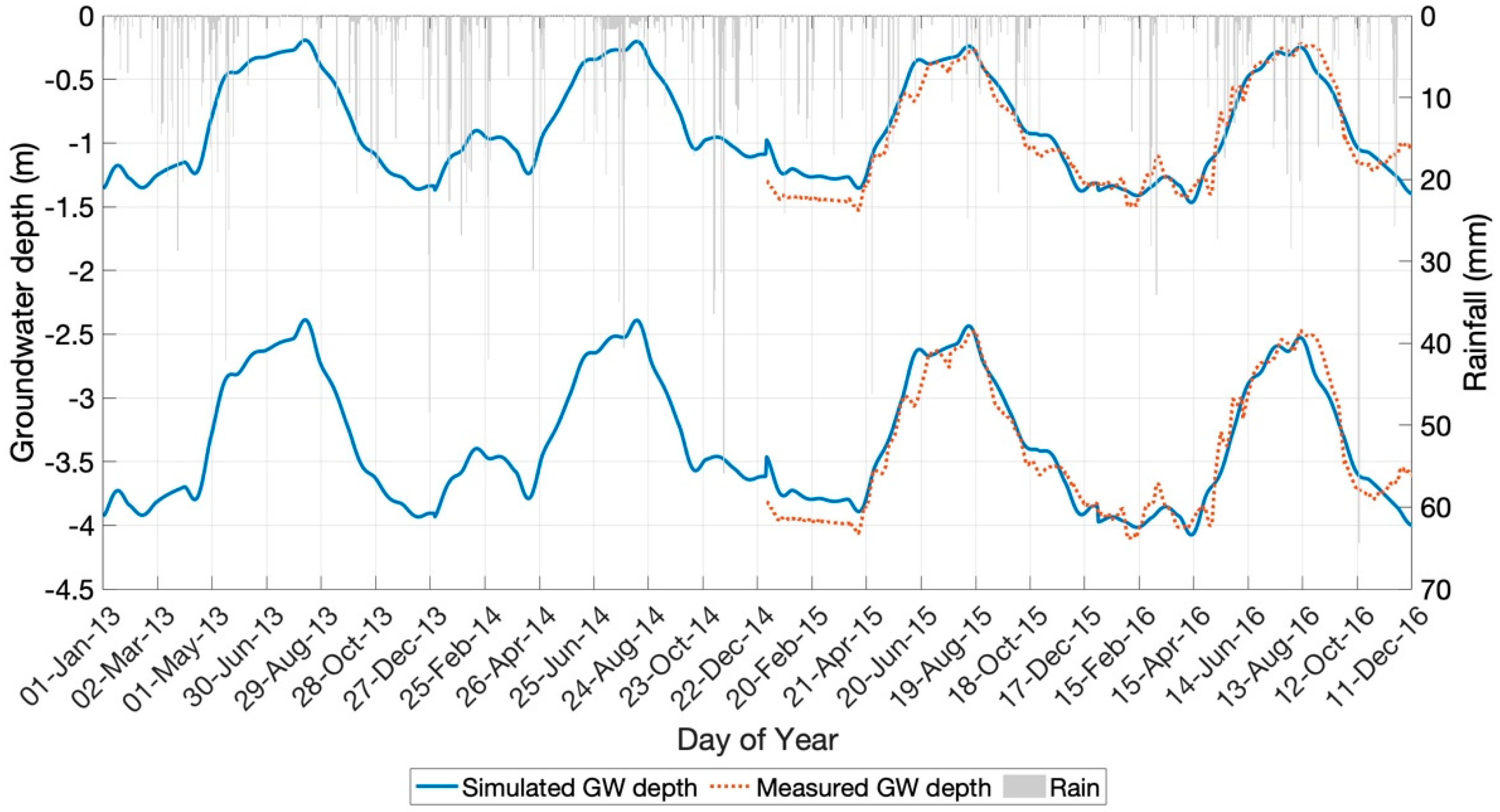
2.2.2. Groundwater Levels

Groundwater levels were measured at weekly intervals by AIES technicians in four piezometers (Figure 2a) installed in the district at the beginning of 2015. Moreover, data series collected at two AIES piezometers located close to the district were also obtained for the period 2013–2016. During two campaigns carried out in July 2015 and 2016, measurements of water level in a deep drainage channel (Bortana channel, represented with a bold line in Figure 2a, together with the point at which water level measures were taken) draining the phreatic aquifer were moreover collected.

A spatial interpolation of measured groundwater depths was computed on a 20 m × 20 m grid for 15 July of each year (2015 and 2016). This date was chosen because it falls in the middle of the summer flooding period, leading to the assumption that the groundwater level has reached its highest value. For the interpolation, groundwater levels at the six piezometers were considered together with water levels measured in the drain, added as ‘fixed points’ (they showed to improve the accuracy of the interpolation obtained). The groundwater table depth from the ground level was computed by subtracting the interpolated groundwater surface from the DEM (Digital Elevation Model, 20 m × 20 m grid, source: Geoportale Nazionale Regione Lombardia). The obtained layer was used to divide the district into two sub-areas, one characterized by a shallow groundwater depth (less than 1 m on 15 July) and the second by a deeper groundwater table. In the two zones, a strong and a negligible influence of groundwater table on percolation and capillary fluxes (this last flux only outside of the flooding period) are respectively expected. Figure 2a shows the two zones as identified for the year 2015, along with the actual groundwater table depth computed starting from the 15 July 2015 data. The same zonation activity was carried out for the date of 15 July 2016. As shown by Figure 2a, interpolated maps (only the one obtained for 15 July 2015 is illustrated) show two very different conditions over the district: about 2/3 of the district area is characterized by a deep groundwater level (dashed area in Figure 2a) with a summer maximum value reaching about 2 m from the soil surface, while the remaining 1/3 (dotted area in Figure 2a) shows a shallower groundwater with a very high summer level (less than 0.5 m from the soil surface). The two areas are due to the presence of territories having a different topographic elevation and are delimited by a very steep surface.

Successively, the interpolation was carried out for each day of the period 2015–2016. For each day, groundwater table depths were averaged over the two zones identified (‘shallow’ and ‘deep’ groundwater) to obtain daily time series for the two zones. Figure 2b shows the obtained time series in the case of the year 2015.

2.2.3. Soil Hydraulic Properties

The available soil map ([17]; scale 1:50,000) shows thirteen different soil units within the district area, but five of them are largely prevalent; their main features are reported in

Table 1. Soil properties of the five prevalent soil units (407–417) within the pilot irrigation district [17]. For each horizon, the upper and lower limit, the sand, silt and clay content and the textural class according to USDA soil taxonomy are reported (LS: loamy sand; SL: sandy loam; S: sand; L: loam).

Unit	Soil Depth	Sand	Silt	Clay	Texture
	cm	%	%	%
407	0–25	76.6	18.2	5.2	LS
	25–50	61.4	25.1	13.5	SL
	50–75	61.2	24.1	14.7	SL
	75–105	86.0	8.0	6.0	LS
	105–120	84.6	12.8	2.6	LS
409	0–40	84.4	10.9	4.7	LS
	40–67	89.1	7.6	3.3	S
	114–150	47.7	43.6	8.7	L
	192–228	92.9	4.9	2.2	S
410	0–25	65.1	30.6	4.3	SL
	25–40	52.2	36.3	11.5	SL
	40–70	43.5	41.5	15.0	L
	70–100	52.0	42.2	5.8	SL
	100–160	81.8	16.5	1.7	LS
413	0–22	54.0	33.0	13.0	SL
	22–29	65.0	21.0	14.0	SL
	29–60	74.0	15.0	11.0	SL
	60–104	93.0	0.0	5.0	S
	104–117	85.0	12.0	3.0	LS
	117–157	98.0	0.0	2.0	S
417	0–35	67.5	28.0	4.5	SL
	35–40	60.7	33.3	6.0	SL
	40–85	63.2	31.7	5.1	SL
	85–140	57.2	33.1	9.7	SL

. The smaller units were merged with the most similar among the prevailing ones.

In order to better characterize paddy soils, a detailed soil survey was conducted in a nearby rice farm characterized by soils similar to those found in the pilot district [10]. Undisturbed soil samples taken at different depths from five soil profiles were analyzed, and for each soil sample texture and retention properties were determined. For each profile, large undisturbed soil cores (height 15 cm, ø 14.6 cm, two replicates) were collected from the less conductive layer (LCL) and taken in the laboratory for the determination of the saturated hydraulic conductivity (Ks) by applying the core method [18]. The measured soil physico-chemical and hydrological properties were used to select the most suitable pedo-transfer function (PTF hereafter) set among those available in the literature to compute soil hydrological parameters from data in Table 1.

The PTF set developed in [19] was selected to estimate the parameters of the van Genuchten-Mualem retention curve [20] for each soil horizon of the five soil profiles. This PTF set requires the following input data: soil horizon texture parameters (percentages of sand, silt and clay), organic carbon content, soil bulk density (BD) and information about the soil structure (size, type and degree of development). Since BD values were not provided by ERSAL [17] (Table 1), fourteen PTF equations to retrieve BD were tested against laboratory-measured values (53 samples collected in this and in previous studies conducted in paddy areas). Since none of the explored PTF equations showed to provide affordable results in the case of paddy soils (Nash–Sutcliff Model Efficiency coefficients were negative in all cases), a simple equation was developed to correct BD values computed by the PTF equation furnishing the least worst results, which was the one developed by [21] for Brazilian hydromorphic and paddy soils. As a matter of fact, in the case of this PTF equation, the plot of measured versus the estimated data showed a clear linear trend but an underestimation of the measured BD values, probably due to the fact that the database used by Tomasella and Hodnett (T&H) was mainly composed by clayey soils. The empirical correction equation (Equation (1)) was applied on the results obtained by means of the T&H PTF (Equation (2)), as follows:

$$\mathrm{BD}=\{\begin{array}{cc}1.2980{\mathrm{BD}}_{\mathrm{T}\&\mathrm{H}}& \mathrm{with} \mathrm{sand}\le 70\%\\ 4.4876-1.9511\times {\mathrm{BD}}_{\mathrm{T}\&\mathrm{H}}& \mathrm{with} \mathrm{sand}>70\%\end{array}$$

(1)

$${\mathrm{BD}}_{\mathrm{T}\&\mathrm{H}}=1.578-0.054\times \mathrm{OC}\%-0.006\times \mathrm{Silt}\%-0.004\times \mathrm{Clay}\%$$

(2)

The Ks values measured in laboratory for the LCLs (5 samples) were far lower than those estimated by applying the PTF suggested in [19]; the average reducing factor was 0.011. This may be explained by the physical and biological clogging processes characterizing paddy soils. Due to the low number of Ks laboratory measurements available, and to the fact that they were conducted on samples taken from the LCL, in this study we decided to reduce Ks of the LCL of each profile by applying the reducing factor, while for the other horizons Ks values were those predicted by the PTF set developed in [19]. The original values predicted by the PTFs are reported in

Table 2. Parameters of the Van Genuchten (θr, θs: residual and saturated water contents; α: air-entry pressure; n: pore-size distribution) and the Mualem-VG (λ: empirical pore-connectivity parameter; Ks: saturated hydraulic conductivity) curves [20], for each soil unit and horizon reported in Table 1, as estimated by the PTFs in [19]. The bulk density (Equation (1), obtained by modifying BD_T&H) is reported in the first column. Values in brackets denote modified LCL Ks values, obtained by applying the 0.011 reducing factor.

Unit	Soil Depth	BD	θr	θs	α	n	λ	Ks
	cm	g cm−3	cm3 cm−3	cm3 cm−3	cm−1	-	-	cm day−1
407	0–25	1.74	0.0000	0.3348	0.0169	1.2859	0.2859	13.86
	25–50	1.77	0.0000	0.3226	0.0111	1.1940	0.1940	89.20
	50–75	1.77	0.0000	0.3220	0.0154	1.1610	0.1610	88.82 (0.97)
	75–105	1.55	0.0000	0.4034	0.0244	1.8436	0.8436	109.61
	105–120	1.58	0.0052	0.3926	0.0688	1.1940	0.1940	114.48
409	0–40	1.65	0.0000	0.3686	0.0467	1.1451	0.1451	56.78
	40–67	1.54	0.0008	0.4071	0.0467	1.3479	0.3479	365.84
	114–150	1.65	0.0496	0.3675	0.0347	1.1352	0.1352	16.33 (0.18)
	192–228	1.49	0.0537	0.4263	0.0470	1.6820	0.6820	283.34
410	0–25	1.72	0.0000	0.3400	0.0295	1.1053	0.1053	1.31
	25–40	1.69	0.0043	0.3537	0.0186	1.2098	0.2098	22.52
	40–70	1.63	0.0447	0.3761	0.0261	1.1365	0.1365	14.15 (0.15)
	70–100	1.68	0.0584	0.3562	0.0318	1.1319	0.1319	27.01
	100–160	1.62	0.0401	0.3769	0.0877	1.1940	0.1940	225.56
413	0–22	1.65	0.0453	0.3660	0.0697	1.1073	0.1073	2.71
	22–29	1.78	0.0000	0.3194	0.0295	1.1940	0.1940	28.86 (0.32)
	29–60	1.68	0.0541	0.3558	0.0336	1.0772	0.0772	132.60
	60–104	1.46	0.0252	0.4397	0.0634	1.6115	0.6115	214.05
	104–117	1.57	0.0000	0.3961	0.0571	1.9240	0.9240	263.97
	117–157	1.43	0.2235	0.4510	0.1660	1.1940	0.1940	28.78
417	0–35	1.72	0.0000	0.3420	0.0301	1.0922	0.0922	1.03
	35–40	1.74	0.0000	0.3346	0.0091	1.2955	0.2955	37.58 (0.41)
	40–85	1.77	0.0000	0.3239	0.0162	1.0704	0.0704	136.27
	85–140	1.73	0.0000	0.3389	0.0122	1.2200	0.2200	47.83

, LCL modified Ks values are shown in brackets.

2.2.4. Land Use Maps and Irrigation Management

Yearly land use maps produced by ERSAL (SIARL—Lombardy Regional Agricultural Information System; 2003–2018), which describe the spatial distribution of major crops in Lombardy on a 20 m × 20 m grid were obtained for the period 2013–2016. To incorporate information on irrigation methods adopted for the different crops, the procedures described below were followed.

According to information provided by AIES, poplar in the area is typically irrigated for the first four years after transplanting (young poplar), while it is rainfed during the successive six years of the productive cycle (mature poplar). Accordingly, poplar areas within the district were randomly split into young and mature, following a 40–60% ratio; since the poplar area in the pilot district is very limited, this choice should not have significant consequences on the simulation results. When irrigated (young poplar), border irrigation is applied 2–4 times a year, with an average irrigation depth of 200 mm.

Maize is usually irrigated by border irrigation, irrigation service is provided by AIES on a rotational basis every 15 days, and an average irrigation depth of about 150 mm is applied. However, in areas of the district having shallow groundwater, farmers adopt a practice to limit the water logging within the fields, since maize plants are sensible to this condition. Fields are divided in narrow sectors by means of earth bunds, and each sector is equipped with inlet and outlet gates. Water level is raised in the irrigation channel, then the inlet gate of the sector is opened and closed again after a while to cut the incoming discharge. This allows a fast water wave to run along the sector exiting the field through the sector outlet. As a consequence, water that effectively infiltrates the soil is supposed to be smaller than the input water discharge, with a portion of that water returning to the drainage network.

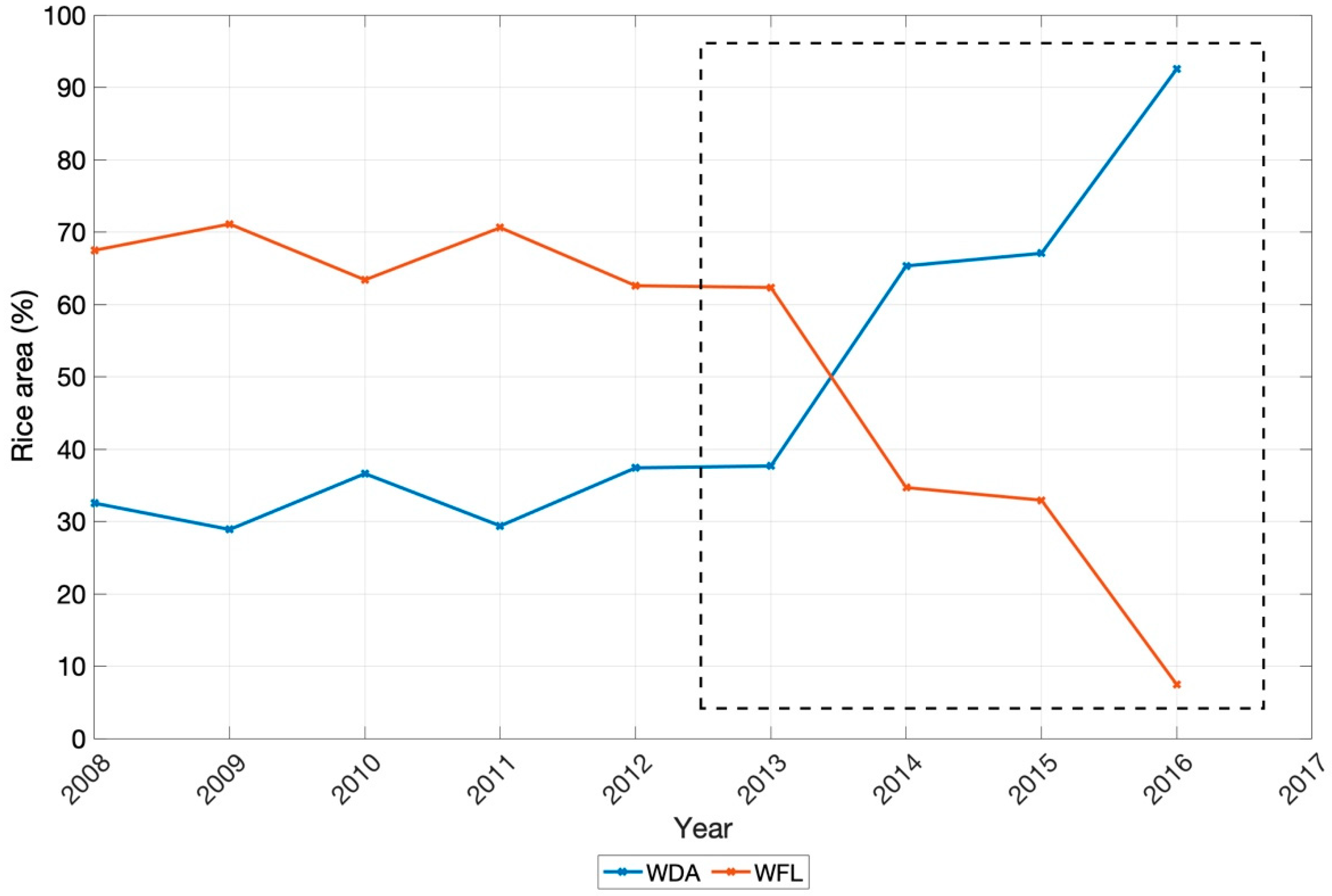
According to statistics provided by ENR, in the district the traditional rice irrigation method (wet seeding and continuous flooding, WFL) has gradually been replaced by a rough version of the alternate wetting and drying irrigation method after dry seeding (WDA) in the last ten years, as shown in Figure 3. This method is adopted with an average rotational schedule of 9 days from the beginning of June to about mid-August. According to AIES, the change in irrigation method was accelerated in the last years by a reduction in the availability of water discharges diverted by AIES and distributed over the district; this was particularly evident starting from 2015 (Figure 4). For the study, it was crucial to identify rice fields irrigated with WFL and with WDA. Randomizing the type of rice irrigation management over the district was not an option in this case, due to the wide surface cropped with rice and to the fact that the coarser soils are those on which farmers most likely practice WDA. Therefore, satellite images (NASA Landsat 7 and 8 missions, spatial resolution 30 m, temporal resolution 16 days and, starting from mid-2015, ESA Sentinel 2 mission, spatial resolution 10 m, temporal resolution 10 days) within the time window extending from half April to the end of May (when flooding starts under WFL and ponding water is still detectable in satellite images because it is not covered by the crop canopy) were downloaded for 2015 and 2016. Due to the high cloudiness conditions that characterize springs in northern Italy, only two non-cloudy images were available in 2015 and none in 2016. The MNDWI index (Modified Normalized Difference Water Index: difference between green and medium-infrared spectral bands over their sum; [22]), which is able to clearly distinguish water from land, was computed for the two images. Areas flooded in the two consecutive images were assigned to the WFL irrigation management. The results for 2015 were encouraging, since well in line with statistics provided by ENR. According to ENR, during 2015, 67% of rice area in the whole San Giorgio district (eastern and western, about 1500 hectares) was irrigated by WDA (Figure 3), while the value found through the satellite image analysis over the same area was 69%. This allowed on one hand to validate the approach based on satellite images implemented, and on the other to verify the reliability of ENR statistics. A random reduction of pixel irrigated by WFL in the 2015 map was applied to obtain the 2016 map, in which rice irrigated by WFL method was 7% in ENR statistics. The same procedure, but with the addition of WFL rice pixels within the whole rice area, was applied for years 2013 and 2014 (WFL 38% and 65% according to ENR statistics).

2.2.5. Water Supply

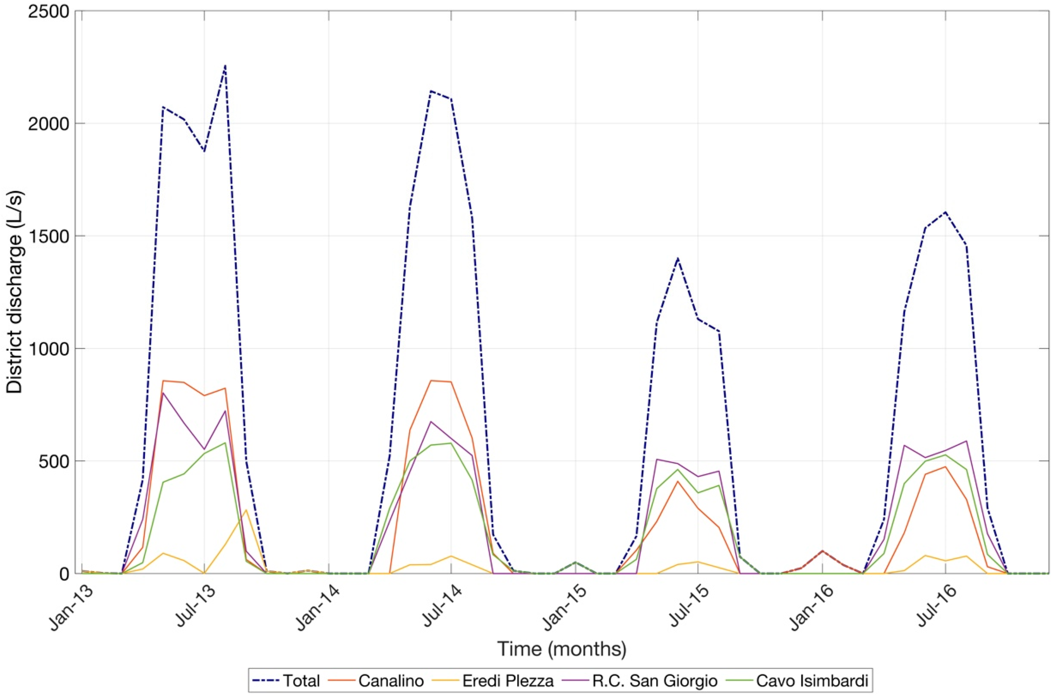
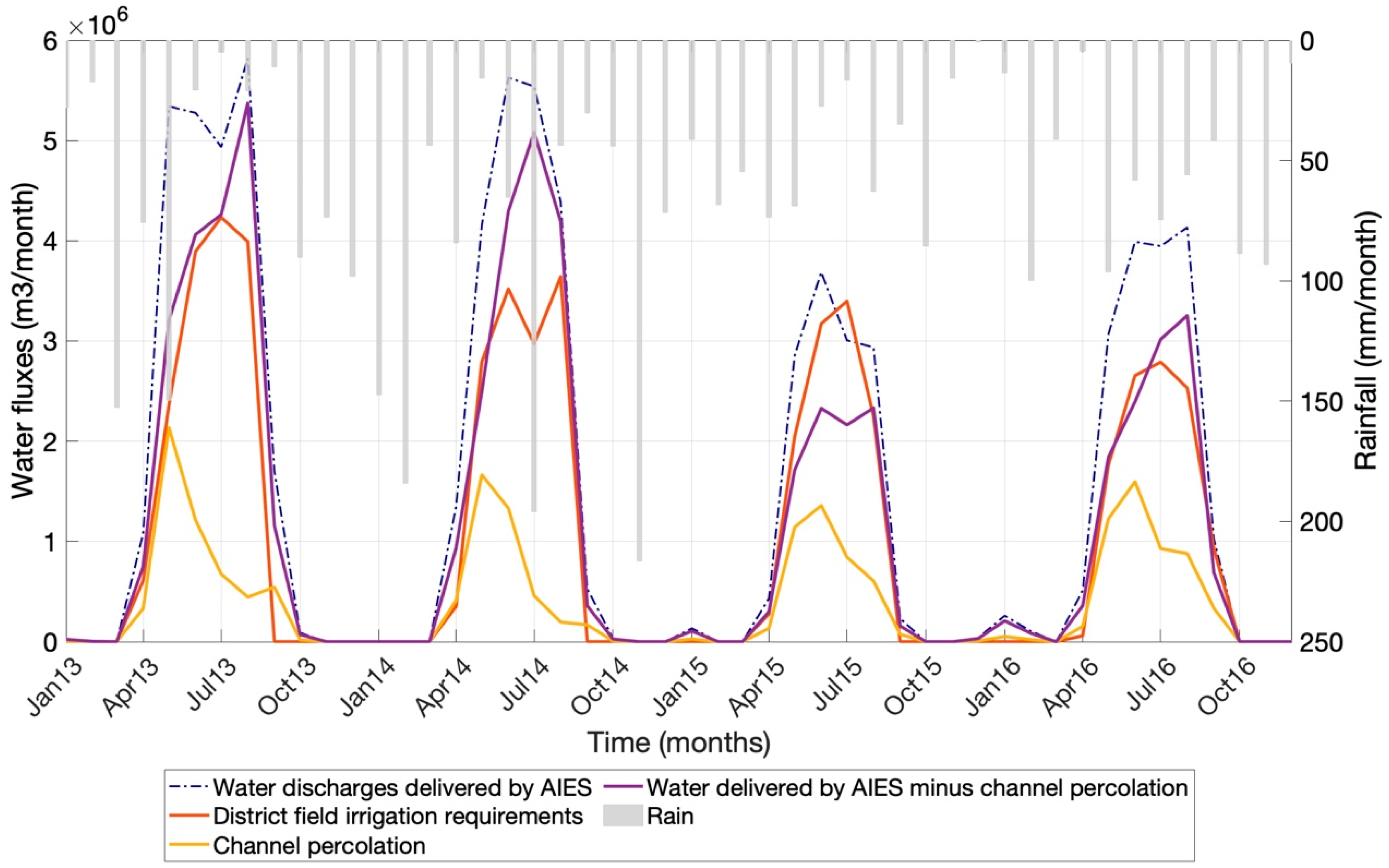
Irrigation water is delivered to the pilot district by four irrigation canals (Canalino, Eredi Plezza, Cavo Isimbardi, and Roggia Comunale di San Giorgio) managed by AIES. Monthly total water discharge conveyed in the period 2013–2016 to the district is shown in Figure 4. Maximum monthly specific irrigation supply rates were respectively 2.2, 2.0, 1.3 and 1.6 L s⁻¹ ha⁻¹ for the four years, while total water volumes delivered to the district in the whole agricultural season (15 April–15 September) were found to be respectively 23.8, 21.2, 13.1 and 16.7 Mm³. Unfortunately, irrigation tailwater discharged by the drainage network downstream of the district and percolation losses from the unlined channel network are not usually quantified by AIES. However, AIES reports irrelevant drainage flows in the central part of the irrigation season, with the exception of days characterized by strong and prolonged rains. Greater drainage flow rates can be observed, depending on the year, at the beginning and at the end of the irrigation season. Percolation losses from the channel network are estimated by AIES to be about one third of the water flowing within the network, with higher rates at the beginning of the season, when the groundwater table is deeper and lower rates at the end of the season, when it is shallower.

2.2.6. Crop Parameters

Information about average sowing and harvesting dates for rice crop over the irrigation district and seasonal patterns of biometric parameters (rice rooting depth, leaf area index, crop height) were provided by ENR technicians. Crop coefficients needed to estimate crop water requirements for different rice irrigation methods were measured in a former experiment carried out in a study site nearby [2,23]. In particular, the following coefficients were observed for three irrigation methods: WFL: Kc_ini = 0.7, Kc_mid = 1.1, Kc_end = 0.6; WDA: Kc_ini = 0.35, Kc_mid = 1.1, Kc_end = 0.6; DFL: Kc_ini = 0.33, Kc_mid = 1.1, Kc_end = 0.6, the last method—dry seeding and delayed flooding—was included in the scenario analysis.

Seasonal patterns of biometric parameters for the maize crop were estimated by applying a growing degree day model calibrated for the main crops of the Po Valley plain [24]; crop coefficients for maize in the plain were measured in a previous experiment [25,26] and the values used are the following: Kc_ini = 0.33, Kc_mid = 1.0, Kc_end = 0.45.

To reproduce the physiological behaviour of maize, a shortening of the maximum rooting length (from 80 to 40 cm) was applied in case of shallow groundwater conditions. For poplar, the generic deciduous forest parametrization suggested in [27] was adopted, due to the lack of specific local information; in the case of young poplars values were corrected by reducing leaf area index, crop coefficient and root length to represent a condition of smaller trees [2].

2.3. Set up of the Modelling Framework

The simulation of water fluxes and storages in the West-San Giorgio (W-San Giorgio) district was carried out following a semi-distributed approach suited to account for the spatial variability of the area. In particular, the simulation system developed and applied in this work is composed by three sub-models: one for the agricultural area, one for the groundwater storage, and one for the channel network.

The semi-distributed model for the agricultural area subdivides the pilot district in zones assumed to be sufficiently homogeneous; each zone (homogeneous sub-unit hereafter), no matter its actual shape and dimension, was described by a specific set of parameters and simulated with a well-known soil-water-atmosphere-plant model (SWAP, [27]). SWAP is used worldwide to simulate vertical (1D) water fluxes and balances in vegetated areas. It is able to handle a number of processes (e.g., water, heat and solutes balances, plant growth) and simulations are highly customizable. SWAP showed good performances even in paddy environments, as reported in previous studies where it had been successfully used to model water dynamics in rice agro-ecosystems [7,28,29,30].

After the simulation, water fluxes simulated in each sub-unit are weighted by the respective surfaces to obtain overall values of the district field percolation and irrigation requirements.

Channel network percolation is estimated on the basis of the irrigation discharge delivered to the district by AIES, as well as of the district groundwater level, through the application of an empirical model. This allows the estimation of the district total percolation and irrigation requirements, respectively computed by adding channel network percolation to the district field percolation and irrigation requirement. In cases in which measured groundwater levels or irrigation discharge delivered to the district are not available, an iterative algorithm is used to estimate the missing data series.

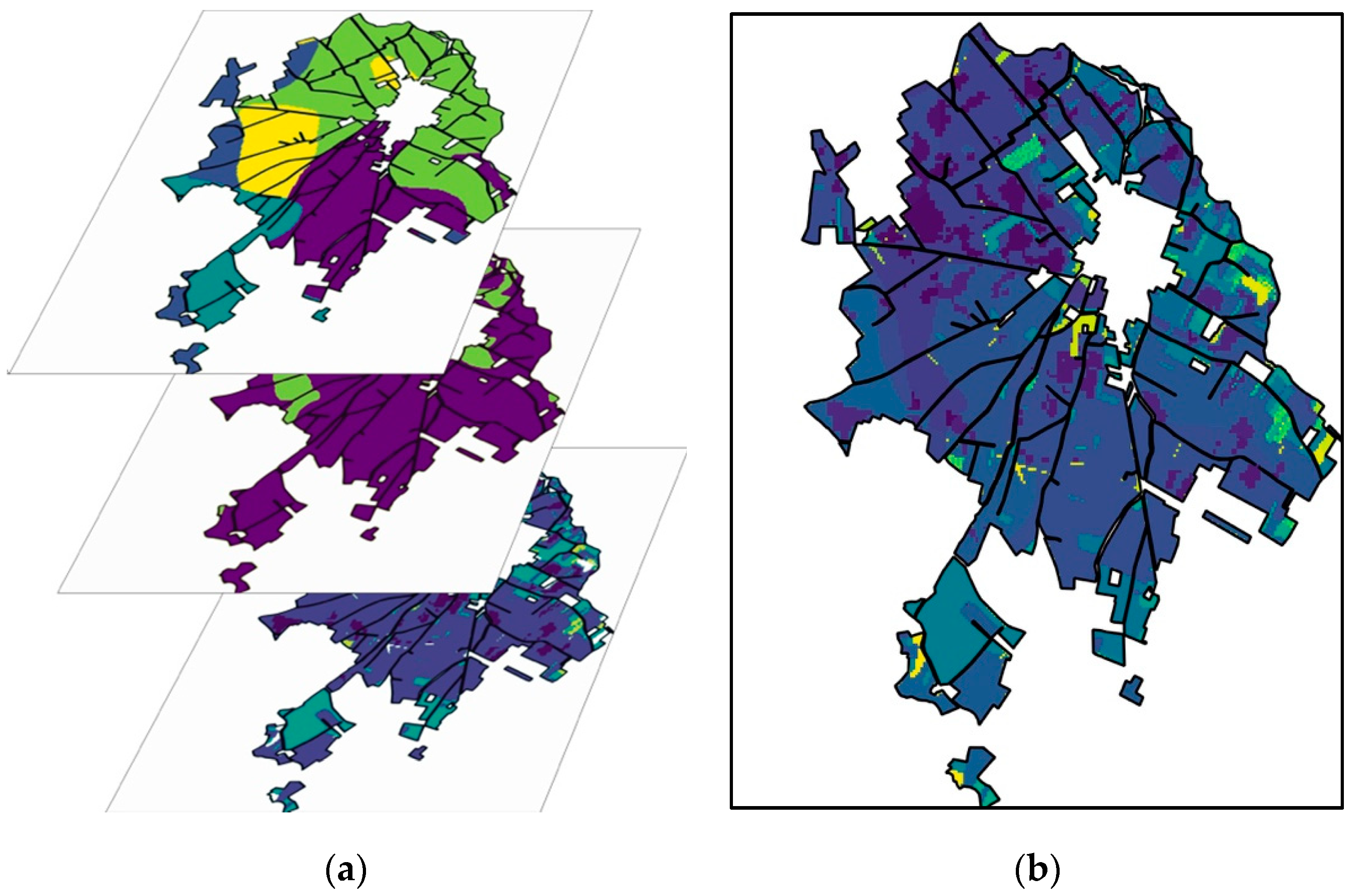
The fifty homogeneous sub-units in which the agricultural area was subdivided were obtained through a map overlying process (Figure 5), by combining soil type, crop type and groundwater level maps; thus, each sub-unit has the same crop type, irrigation method and scheduling, soil unit and groundwater level conditions.

Interactions among the three sub-models composing the simulation system are rather complex and depend on the data available for the different simulations, as shown in the flowchart illustrated in Figure 6. Some operations were performed only during the simulation of the ‘present state’ covering the years 2015 and 2016 for which groundwater level (GWL) time series were available. These operations are described in Section 2.3.1 ‘Direct flow path’ and illustrated in the left side of Figure 6. Other operations were carried out only during the simulation of the ‘present state’ for the years 2013 and 2014 and of the ‘hypothetical scenarios’, for which GWL was unknown and needed to be estimated. Steps undertaken in these cases are illustrated in Section 2.3.2 ‘Feedback flow path’ and in the right side of Figure 6.

In order to allow a better representation of the two paths, in Figure 6, operations involved only in the ‘direct flow path’ are dashed, those involved only in the ‘feedback flow path’ are dotted, while solid arrows denote operations common to both paths.

Apart from the soil-plant-atmosphere model (SWAP), that is a standalone model developed in FORTRAN language, the whole simulation system was developed in this study as an original code in MATLAB©R2018b. Model inputs and parameters (describing meteorological data, crops, soil, irrigation management, etc.) were provided to the simulation system through Excel files, while outputs were printed in MATLAB© (mat) files and then analysed within the MATLAB© environment. As already introduced, the simulation system includes the SWAP model and two empirical models accounting for channel percolation (Section 2.3.1.1 and Section 2.3.2.1) and groundwater dynamics (Section 2.3.2.2). The ‘direct flow path’ shown in Figure 6 is explained in detail in Section 2.3.1, while the ‘feedback flow path’ is illustrated in Section 2.3.2 introducing only novelties and differences with respect to the ‘direct flow path’.

2.3.1. Direct Flow Path

In the years 2015 and 2016, GWL data series were measured in different locations (Figure 2). At the beginning of the simulation, the system performs the operations described in Section 2.2.2 to subdivide the pilot district in two zones having shallow and deep groundwater table levels (‘Zonation’ in Figure 6) and to produce the corresponding groundwater table depth series (respectively ‘GWTs’ and ‘GWTd’ in Figure 6).

The core of the simulation system is illustrated in Figure 6 as a pile of rectangles representing the ensemble of SWAP simulations carried out for each of the 50 homogeneous sub-units in which the pilot district study area was subdivided along with its input and output data. For each sub-unit, the system reads the whole set of inputs and parameters from the Excel files (including the GWL dataset produced in Section 2.2.2), properly formats data within the text files required to run SWAP, calls SWAP to run the simulation, collects the simulation outputs and stores them in a MATLAB© file.

The results of the 50 SWAP runs were aggregated on the basis of the surface covered by each sub-unit to calculate district water balance terms (‘Analysis and spatialization’ in Figure 6). In particular, monthly volumes of district field irrigation requirements, percolation and evapotranspiration fluxes from agricultural areas were calculated. Average monthly values of measured GWLs and irrigation discharge delivered to the district by AIES were used to compute monthly channel percolations (Section 2.3.1.1). Total district irrigation requirements for the district (sum of irrigation requirements for the agricultural areas and water losses from the channel network) were then computed and compared with the district water discharges conveyed by AIES to the pilot district. The system composed by the two models was calibrated following what is reported in Section 2.4.1 and Section 2.4.2.

2.3.1.1. Channel Percolation Model

A channel network percolation model was built and calibrated using data of the years 2015 and 2016 to quantify the amount and temporal distribution of water losses during the irrigation season. Irrigation canals in rice areas of northern Italy are usually unlined and, consequently, important water losses take place especially in the first months of the irrigation season, when all the irrigation conveyance and distribution channels are progressively filled with water. To simulate the water exchange between unlined channels and groundwater the following empirical relationship was adopted:

$$Pca{n}_t=Q_t{\alpha }_t$$

(3)

where monthly channel percolation (Pcan, m³) for the t-th month is a function of the mean monthly irrigation discharge provided by AIES to the district (Q, m³) and of a loss factor (α, −), calculated as follows:

$${\alpha }_t=0.2, \mathrm{for} t<4 \mathrm{or} t>9$$

(4)

$${\alpha }_t=min\left(0.4, max\left(0, S_t-1.6\right)\right), \mathrm{for} 4\le t\le 9 (\mathrm{April} \mathrm{to} \mathrm{September})$$

(5)

being S_t the mean district groundwater depth for the t-th month. During the agricultural season, according to Equation (5), α was allowed to vary between an upper limit of 0 (i.e., null average percolation over the district channel network, due to a compensation between network portions draining and feeding the phreatic aquifer) and a lower limit of 0.4 depending on the groundwater level, while it was set to 0.2 outside the season (Equation (4)), when smaller distribution channels are commonly dry.

2.3.2. Feedback Flow Path

In case of non-monitored GWL data, the simulation system couples a recursive computation with the ‘direct flow path’ approach, by following the steps schematically described here and better detailed in the rest of this Section: (1) it provides a first version of tentative mean daily GWL series or the whole district, from which the two GWL series (‘deep’ and ‘shallow’) are built; (2) it calculates the district total percolation; (3) it applies the empirical GW-percolation model obtaining a new monthly GWL series; (4) it averages the newly obtained GWL series with the previous one; and (5) it goes back to step 2 until a convergence is reached.

As explained in point (1), a tentative daily GWL series is provided at the beginning of the iterative process. This series is supposed to be the mean value of the GWL over the whole district. From this series, the two needed GWL series (‘GWTs’ and ‘GWTd’) are obtained through a number of steps. In particular, a map reporting for each cell (grid 20 m × 20 m) the difference between the interpolated value of GWL at the 15 July and the value for the same day of the mean input GWL series is calculated. This map (called ‘difference map’ hereafter) shows how the GWL in each cell varies with respect to the mean district value; the GWL on the district is assumed to vary during the year by maintaining this difference as a constant. The ‘difference map’ is therefore used to produce a spatially distributed map of GW depths starting from the daily GWL series. Subsequently, in each iteration, the zonation method proposed for the ‘present state’ simulation (threshold of 1 m of depth on 15 July) is applied in order to subdivide the district in ‘shallow’ and ‘deep’ areas. Two new GWL series are then dynamically created by averaging the GWL values of cells belonging to each area for each day of the year; these two series are then used as input for SWAP model as in the ‘direct flow path’.

After the calculation of the total district percolation (from agricultural areas and channel network; for this last flux see Section 2.3.2.1), another empirical model is applied to estimate the groundwater level (Section 2.3.2.2). Finally, output GWL and initial GWL series are averaged and given as input in the next iteration (i + 1). A few iterations (4 to 6) are generally sufficient to obtain stable GWL series, whatever is the tentative GWL series used to start the process. In order to test the procedure, the ‘feedback flow path’ was applied to obtain GWL data series for years 2015 and 2016, and the simulated GWL series were compared to the measured ones.

2.3.2.1. Channel Percolation Model

In case of ‘feedback flow path’, the channel percolation needs to be computed without knowing the irrigation discharge supplied to the district $Q_t$. This can be solved by considering the total irrigation discharge being equal to the total district irrigation requirement:

$$Q_t=I_t+Pca{n}_t$$

(6)

where $I_t$ and Pcan_t are the district field irrigation requirement and the channel network percolation of the t-th month. By using Equation (3):

$$\frac{Pca{n}_t}{{\alpha }_t}=I_t+Pca{n}_t$$

(7)

and solving for $Pca{n}_t$ the following is obtained:

$$Pca{n}_t=\frac{{\alpha }_t\times I_t}{1-{\alpha }_t}$$

(8)

2.3.2.2. Percolation-Groundwater Level (PGL) Model

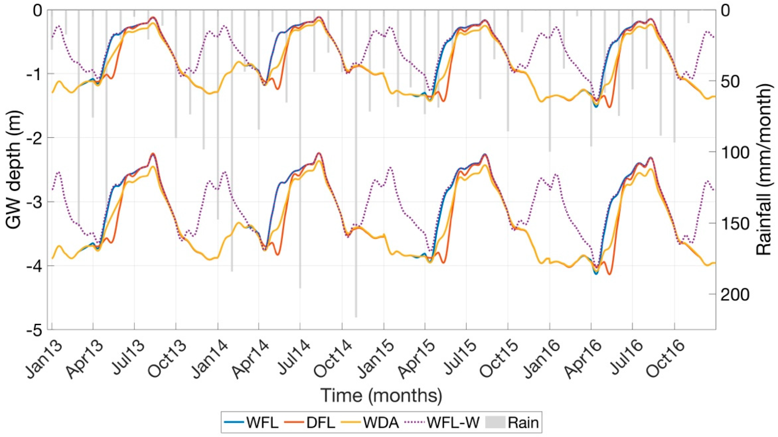
A first attempt at an empirical model connecting observed monthly mean GWL and estimated percolation, both at the irrigation district scale, was presented in [2]. In that case, the relationship between district percolation and GWL (measured in a single agricultural well and considered representative for the whole district area) showed a parabolic behaviour.

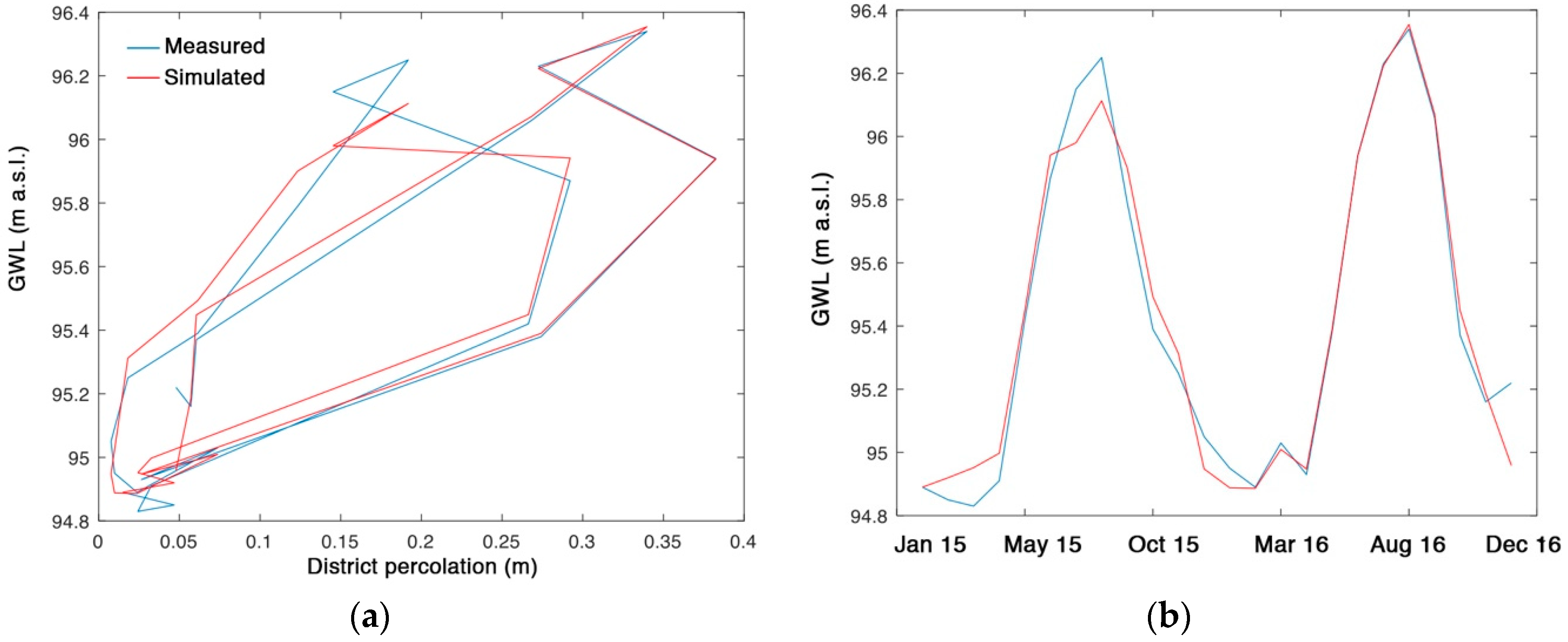
For the western part of the San Giorgio district, different models were tested in order to select the one better suited to interpret the 2015 and 2016 datasets. For both years, monthly values of district percolation versus GWL were found to be positioned on circle-like structures which are followed anticlockwise (Figure 7a). This means that changes in percolation come before changes in GWL, with an inertia in GWL clearly due to a memory effect. Models initially tested were deterministic and had at least an autoregressive term (αy_t−1, accounting for the memory of the aquifer), an exogenous term (βP_t, recharge through percolation), and a constant (γ, avoiding level reaches 0 m a.s.l.). The following models were checked: simple autoregressive, second order regressive and two linear reservoirs in cascade (one for the soil and one for the subsoil). However, they were unable to reproduce the increase in the GWL occurring in July as it corresponds to a decrease in the estimated percolation, occurring in both years (Figure 7b).

To reproduce this behaviour, a GWL data series measured in an agricultural well positioned upstream of the irrigation district along the main groundwater flux direction was taken into account in the model (Cascina Stella, located about 4 km NNE from the centre of the district, shown in Figure 2a). In this way, water stored in the aquifer within the pilot district depends both on the district total percolation recharge, and on the groundwater flux entering the district from upstream, indicating that the district phreatic aquifer is not hydrologically isolated.

The chosen model has the following form:

$$y_t=\left(1-\delta \right)\times \left(\alpha y_{t-1}+\beta \times P_t+\gamma \right)+\delta \times R_t$$

(9)

where t is the monthly time index, y (m a.s.l.) is the GWL averaged in the month and over the district area, P (m) is the total monthly district percolation (estimated by the simulation system), R (m a.s.l.) is the regional upstream GWL (measured at Cascina Stella), α (−) is the memory of the system (connected to the amount of water of the previous month that is still available in the current month), β (−) is the increase in GWL due to 1 m of percolation, γ (m a.s.l.) is the height of the bottom of the system, δ is the weight of the influence of the regional GWL on the district GWL.

The PGL model works at a monthly time step, while the timestep of GWL series needed as input for SWAP is daily. The cumulation of daily district percolations in order to obtain a monthly district time series to feed the PGL model was easy, while it was more complicated to generate daily GWL time series to feed SWAP from monthly estimations produced by the PGL model. To solve the issue, the following approach was implemented, by recurring to an ad hoc set of 4th order polynomial curves (SP4 hereafter). For each month (supposed to be 30 days long), the five parameters of the SP4 were obtained by solving a linear equations system containing the following conditions:

$$y_n\left(-1\right)=y_{n-1}\left(29\right)$$

(10)

$$y_n\left(29\right)=\left(m_n+m_{n+1}\right)/2$$

(11)

$$\frac{d{y}_n\left(-1\right)}{dt}=y_{n-1}\left(29\right)-y_{n-1}\left(29-1\right)$$

(12)

$$\frac{d{y}_n\left(29\right)}{dt}=\left(m_n+m_{n+1}\right)/30$$

(13)

$$\underset{-0.5}{\overset{29.5}{{\displaystyle \int }}}{y}_n\left(t\right)dt=30\times m_n$$

(14)

where y_n(x) is the value of the SP4 of the n-th month at the t-th day of the month (going from 0 to 29), m_n is the monthly mean given by the PGL model for the n-th month. At the end of December, a null derivative was imposed. Derivatives and the integral were solved analytically. With the conditions reported above (Equations (10)–(14)), the result was rather stable. Tests were conducted comparing observed GWL daily time series and the corresponding one obtained by the SP4 approach fed by monthly averages.

2.4. Calibration of the Modelling System

2.4.1. Semi-Distributed SWAP Model

To simulate irrigation needs of the agricultural area and to reproduce as much as possible the farmers’ behaviour, a manual fine tuning of parameters involved in the field irrigation management (frequency, water volumes, irrigation threshold) for each crop was carried out with the support of AIES technicians. This allowed the fitting of simulated irrigation discharges (obtained by adding irrigation requirement of agricultural areas and irrigation losses from irrigation canals), and measured irrigation discharges actually supplied by AIES to the district in the period 2013–2016. In the calibration, particular attention was given to the good fitting of irrigation discharges in the central months of the irrigation season (June, July, August). Moreover, after the calibration process, irrigation tailwater discharged by the channel network downstream of the district, especially during the initial and final months of the irrigation season and in long and intense rainy periods, was quantified by the model and checked by AIES.

The manual calibration of the irrigation parameters took, for young poplar, to a fixed irrigation schedule with two applications at the beginning and close to the end of the agricultural season, with an irrigation water depth of 150 mm. Maize irrigation was set as on demand, by manually calibrating a threshold giving a number of irrigation events per season in accordance to what reported by farmers; in particular, two different irrigation depths (110 and 180 mm) were selected for shallow and deep GWL areas, respectively. Depending on soil type, this approach led to 2–6 irrigation events in areas with a shallow GWL, while 3–7 events were obtained in areas with deeper GWL.

To simulate traditional rice irrigation (WFL), a daily irrigation amount of 30 mm was delivered continuously from the end of April to the end of August, with the exception of three 4-days intervals, when irrigation was assumed to be interrupted for the application of interventions (fertilizers and pesticides). At the end of each 4 days period, water volume still stored within the field (i.e., not infiltrated) was discharged. Moreover, SWAP was also set to discharge water from submerged paddy fields as long as the water level exceeds a ponding water of 12 cm.

With respect to intermittently irrigated rice (WDA), AIES stated that in condition of good water availability the length of the irrigation turn in a fixed rotational schedule applied within the district is 7 days. This value was implemented for years 2013 and 2014. Due to a lower water availability for irrigation in 2015 and 2016, the irrigation turn was set to 9 days for the first month, and successively to 12 and 10 days respectively, as suggested by AIES. In each irrigation event, a water volume corresponding to 120 mm (for deep GWL areas) and 70 mm (for shallow GWL areas) was provided.

The results of the simulations carried out for years 2015 and 2016 following the ‘direct flow path’ (Section 2.3.1), were then used in the calibration of the empirical models used to simulate channel percolation (Section 2.4.2) and groundwater levels (Section 2.4.3).

2.4.2. Channel Percolation Model

The calibration of the channel percolation model was conducted contemporaneously to the calibration of the irrigation management parameters for the different crops within the agricultural area (Section 2.4.1), and it was mainly based on the information provided by AIES technicians. In particular, the difference between monthly water discharges supplied to the district and district total monthly irrigation requirement (agricultural area plus water losses from the channel network), respectively measured and simulated in 2015, was used for a manual calibration of the groundwater depth at which channel percolation reaches its maximum (1.6 m in Equation (5)). The Nash–Sutcliff Model Efficiency (NSME) index was computed over the whole two-yearly period (2015–2016) as well over the two agricultural seasons (April–September 2015 and 2016).

2.4.3. Percolation-Groundwater Level (PGL) Model

The calibration of model parameters (α, β, γ, δ) was performed using all the available data (2015 and 2016). The four parameters were automatically calibrated (using the algorithm ‘lsqnonlin.m’ applied 1000 times with starting points randomly selected from a uniform distribution covering the feasible range of the parameters, namely: 0.1–1.0; 3.0–5.0; 60.0–94.8 m a.s.l.; 0.0–0.1, respectively for α, β, γ, δ). The posterior distributions of the estimated parameters were tightly wrapped around the mean convergence values giving the following final parameters values: 0.83, 3.20, 13.4 m a.s.l., 0.56, respectively for α to δ. The Nash–Sutcliff Model Efficiency (NSME) for 2015 and 2016 was finally computed.

2.5. Irrigation Management Scenarios

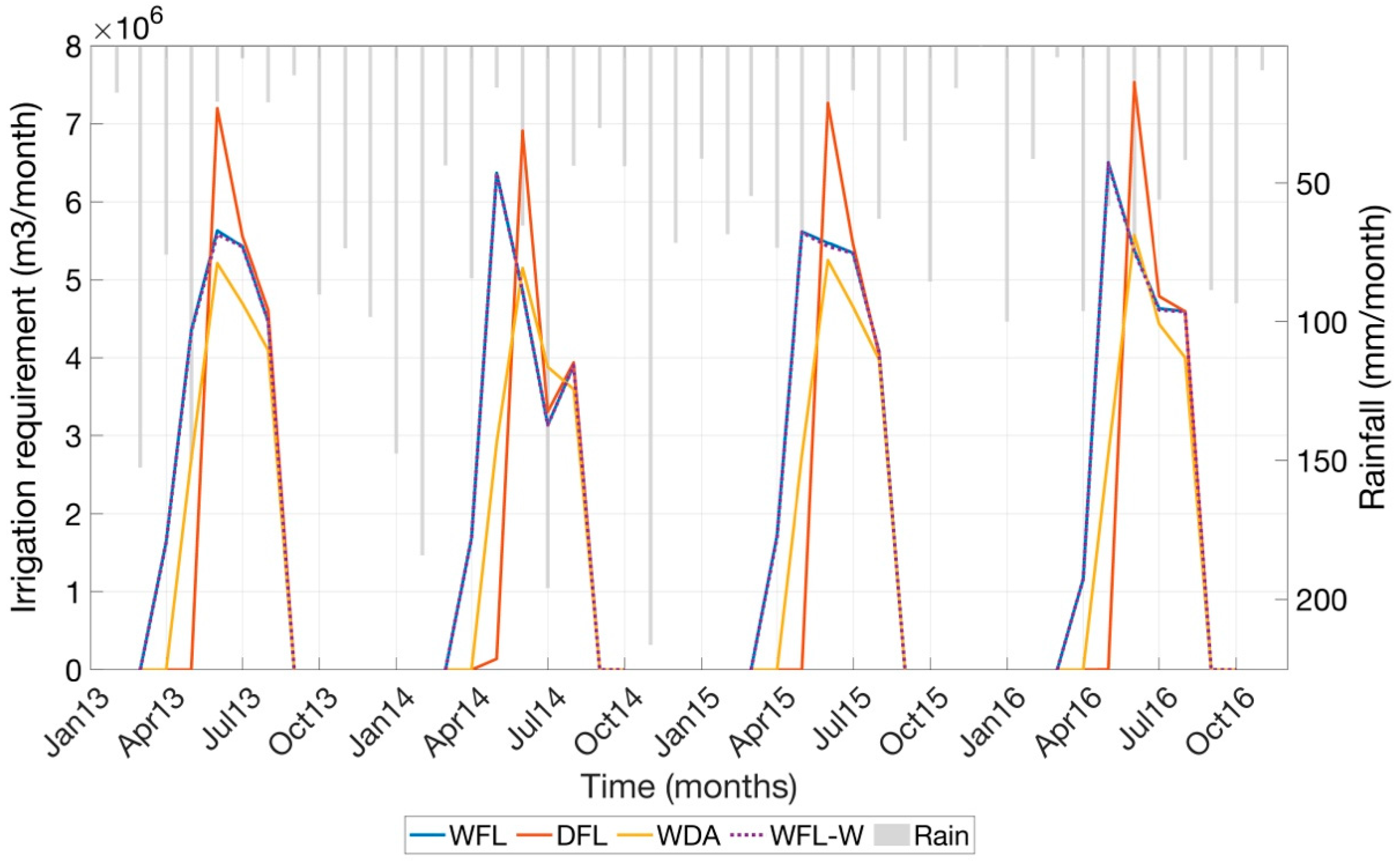
Alongside the assessment of water consumption and water use efficiency in the district in recent years characterized by a strong shift in the irrigation management of rice areas (2013–2016), the objective of this study was to evaluate the effects of massive changes in irrigation water management of rice crop on the district hydrological balance and water requirements. In particular, the following alternative rice irrigation management options were considered and applied to the whole rice area within the district considering agrometeorological data at the Castello d’Agogna weather station from 2013 to 2016: traditional wet seeding and continuous flooding (WFL); alternate wetting and drying irrigation (WDA); dry seeding and delayed flooding condition (DFL); WFL followed by winter flooding (WFL-W).

Options WFL and WDA are already adopted within the district. DFL is quite common in northern Italy, especially in the Lombardy paddy area. The method is characterized by rice sown directly on dry soil, seeds development relying only upon soil moisture for the first three-four weeks, and continuous submersion started when the crop reaches the 3rd–4th leaf stage (in average at the end of May) until almost harvest, excepting for two short periods (four days) in which water inflow is stopped to allow agronomical operations, such as for WFL. The interest in this scenario is to assess if its application in the district could be considered a ‘water saving technique’, not only considering the total seasonal irrigation volume, but also its monthly distribution along the irrigation season with respect to the traditional WFL. The last scenario, WFL-W, involves WFL during the cropping season and winter flooding of paddy fields from 15 November to 15 January. Winter flooding in that period is presently funded by the Lombardy Region RDP 2014–2020 for environmental reasons (improving the biodiversity, mainly maintaining migratory waterfowl habitats).

Scenario analysis was performed by running the modelling system with the same meteorological, crop, irrigation (except for WDA rice irrigation turn that was set to 8 days, an average value suggested by AIES) and soil data as in the current state simulations, but estimating mean GWL through the calibrated GW model following the ‘feedback flow path’ (Figure 6). In order to better discriminate the effects on the district water needs of the different water management options, the same land-use map was used in all the simulations for the entire time period (2013–2016); in particular, the land use map for 2015 was selected. With the exception of the rice crop, for the other crops (i.e., maize, poplar) the irrigation methods implemented in the ‘current state’ simulations were maintained.

2.6. Computation of Water Use Efficiency and Channel Efficiency

Water use efficiency (WUE, %) was calculated according to [3]:

$$\mathrm{WUE}=\frac{\mathrm{E}+\mathrm{T}}{\mathrm{I}+\mathrm{R}}\times 100$$

(15)

where E, T, I and R (evaporation, transpiration, irrigation and rainfall, respectively) are expressed as total volumes (m³) over the agricultural season (15 April–15 September). Evaporation, transpiration and irrigation fluxes were calculated (in mm) for all the homogeneous sub-units through the application of the semi-distributed modelling approach presented in this paper, and then weighted by the sub-unit surfaces to obtain the total volumes in m³.

Channel efficiency (CE, %) was computed as the ratio between the water volume effectively delivered to agricultural fields and the water volume diverted from surface irrigation water sources:

$$\mathrm{CE}=\frac{\mathrm{Qdelivered}}{\mathrm{Qconveyed}}\times 100$$

(16)

3. Results and Discussion

3.1. Current State (2013–2016)—Water Balance and WUE

3.1.1. Overall District Values

Figure 8 illustrates the results for the ‘current state’ simulations (2013–2016), obtained following the ‘feedback flow path’. The measured fluxes shown in the figure are rainfall and irrigation water delivered to the district, while the simulated ones are channel percolation, district field irrigation requirement, and available irrigation water at the field level (i.e., irrigation supply minus channel percolation). For what concerns the accuracy of the channel percolation results, the Nash–Sutcliff Model Efficiency (NSME) computed over the whole period 2015–2016 was found to be 0.67, reaching 0.8 when considering the agricultural period characterized by the major channel water losses, namely April to July.

The estimated district total irrigation requirement is well in line with the available irrigation water at the field level for the years 2013 and 2016, except for the month of August, where a high irrigation supply often coexists with decreased evapotranspiration, increased rainfall, and higher GWL compared to the previous months (especially July). As a consequence, the simulation system estimates irrigation tail-water discharges in August of the two years, calculated as the available irrigation water at the field level minus the district field irrigation requirement. The same applies for the central months of the 2014 agricultural season, where an exceptional rainfall amount (430 mm, mainly concentrated in July 2014, compared to 260 mm in 2013) led to abundant water availability, to a decrease in district field irrigation requirement and thus to copious irrigation tail-water. Conversely, the year 2015 was characterised by lower water discharges conveyed to the district (13 Mm³ from the 15 April to the 15 September, versus 24 and 21 Mm³ in 2013 and 2014, respectively) and to a rather dry summer (rainfall amount of 275 mm). For that year, the simulation system estimates an irrigation requirement higher than the actual water supply. As a matter of fact, according to AIES, in 2015 district farmers experienced production losses due to water scarcity.

In Figure 9 the GWL series estimated for the period 2013–2016 following the ‘feedback flow path’ is compared with the GWL measured in 2015 and 2016. In the figure, data series for both shallow and deep GWL zones are shown. A good overlay of the two series was generally obtained, with the exception of the beginning and the end of the calibration period, for which measured data were probably of worse quality; however, the overall fitting during the agricultural seasons was judged to be very satisfying. The NSME index averaged over the two GW series (‘GWTs’ and ‘GWTd’) was 0.89 when calculated for the whole two-year period, while it reached 0.98 when considering only the agricultural season (15 April–15 September) of the two years. Thanks to this, the model was expected to provide reliable results also for situations in which GWL measures were not available. Figure 9 shows that during the first years of the data series, characterized by a greater presence of flooded rice, GWLs rise earlier during the irrigation season and reaches higher values compared to the last years of the series. Vice versa, in the last years, characterized by an increased presence of intermittently irrigated rice, GWLs rise later in the season, the peak due to summer flooding is narrower, and the reached levels are slightly lower than those simulated for the first years. The behavior of groundwater levels are shown to be different from year to year in the late autumn/winter/spring seasons, depending heavily on the quantity and distribution of rainfall.

In the remaining part of the Section, only the results for the period 15 April–15 September of 2013 and 2016 are analysed in detail, since these two years showed the largest difference in terms of paddy irrigation management (i.e., 62% WFL and 38% WDA in 2013, and 7% WFL and 93% WDA in 2016), and were characterized by almost average values of rainfall totals during the summer season. Besides, results for 2014 are hardly comparable to other years due to the exceptional rainfall amount in the summer season, while for 2015 some underestimation possibly present in water deliveries data could affect the results (the amount of water provided to the district was dramatically low if compared with the previous years, as shown in Figure 8).

District total irrigation requirements (irrigation from agricultural areas plus channel percolation) are found to be 20.5 Mm³ and 15.8 Mm³ for the years 2013 and 2016, respectively. The important decrease in the irrigation requirement can certainly be attributed mainly to the massive change in rice irrigation management observed over the district from 2013 to 2016; however, rainfall during the central part of the agricultural season 2016 (219 mm from June to September versus 69 mm in 2013) probably played a certain role in reducing the district field irrigation requirement. WUE calculated for the agricultural area shows only a moderate increase (6%) from 2013 to 2016 (

Table 3. District total irrigation requirements (Irrig. Req.), water use efficiency of the agricultural area (WUE) and channel network efficiency (CE), calculated for the whole 2013 and 2016 agricultural seasons and for the month of July. WUE values for shallow and deep groundwater zones are reported in brackets. WFL and WDA express the share of traditional wet seeding and continuous flooding and wetting and drying alternate irrigation management over the district, respectively.

Year	Paddy Irrigation Management	Irrig. Req. (Mm3)	Irrig. Req. July (Mm3)	WUE (%)	WUE July (%)	CE (%)	CE July (%)
2013	62% WFL, 38% WDA	20.5	4.9	30 (37, 27)	37 (45, 33)	78	86
2016	7% WFL, 93% WDA	15.8	3.7	36 (46, 32)	42 (55, 37)	69	77

; WUE values for shallow and deep groundwater zones are reported in brackets). In contrast with the irrigation needs and the WUE of agricultural areas, channel network efficiency shows a decrease from 2013 to 2016, justified by a lower GWL due to the reduction of percolation from agricultural areas caused by the change in the irrigation management. Similar differences between 2013 and 2016 can be observed also when considering the month of July, which is the most critical for irrigated systems in northern Italy.

3.1.2. Land Use and GWL Zones Results

Water balance terms referred to the different land use types computed as an average of the 2013–2016 period are reported in

Table 4. Average water balance terms resulting from simulations and WUE of the agricultural area referred to the different land use types calculated for the cropping season (15 April–15 September) for the period 2013–2016. WUE averaged over areas characterized by shallow and deep GWLs are reported in brackets; average rainfall value was 320 mm.

	Actual Evapotranspiration (mm)	Irrigation (mm)	Percolation (−) or Capillary Rise (+) (mm)	WUE (%)
Maize	449	620 (438, 705)	−589 (−243, −732)	50 (61, 44)
Irrigated poplar	348	300 (300, 300)	−247 (−215, −252)	57 (50, 58)
Rainfed poplar	487	0	−18 (+232, −57)	159 (149, 159)
WDA rice	537	1394 (964, 1620)	−1002 (−491, −1206)	34 (43, 29)
WFL rice	592	1852 (1508, 2210)	−1266 (−860, −1693)	28 (32, 23)

. Water fluxes are expressed in mm for each land use unit and are obtained through a weighted average of the fluxes produced by each sub-unit characterized by a certain land use; thus, their values refer to areas with shallow and deep GWLs and different soil types. Vertical fluxes at the bottom boundary of the agricultural soil must be considered as percolation when negative and as capillary rise when positive. Figure 10 shows the pattern of WUE for the three main crops of the district (maize, WDA rice and WFL rice) over the four-year period (2013–2016) respectively for deep and shallow GWL areas.

Table 4 shows that, in the case of WFL rice, an average irrigation value of 1,850 mm is applied over the district. Average values of 1500 mm and 2200 mm are respectively found for shallow and deep GWL areas. The large difference between this estimation and the one provided in [2] for East San Giorgio (E-San Giorgio) irrigation district (3400–4300 mm) is due to the different soil and groundwater conditions: E-San Giorgio is characterized by coarse sandy soils and a groundwater table reaching a maximum value of about 80 cm from the topographic surface in the summer, while the majority of WFL rice in W-San Giorgio is located on soil units presenting heavier soils with impervious layers. Moreover, half of the WFL rice surface is located in areas characterised by a shallow (less than 50 cm from the surface) groundwater table. Furthermore, 1800 mm is well within the range of irrigation requirement values measured in the few studies conducted in Lomellina (e.g., [10]).

Irrigation amounts computed the for maize crop are very different over the years, especially for shallow GWL areas, due to the different timing in summer rain events, and take to an average value over the whole district of 620 mm, while values of 440 mm and 700 mm are respectively found for shallow and deep GWL areas; the simulated values are well in line with those found for the Padana Plain in other studies.

Required irrigation amounts for WDA rice showed an average value of 965 mm for shallow GWL areas and 1600 mm for deep GWL areas. The average value for the district, 1400 mm is not much lower than the average value for WFL (1800 mm). However, it must be considered that, especially during the first years of the period (2013–2014), WDA was initially applied to the coarser soil areas and irrigation turns were particularly short (7 days), thus reducing WDA’s ‘water saving’ potential.

For young poplar, following AIES suggestions, two fixed irrigations of 150 mm were set during the agricultural season, these resulted to be enough to avoid important water deficit stress. Results of the simulations for the single years (not reported) showed that mature poplar, not irrigated, suffered from light water shortage in the central part of the summer season of dryer years (i.e., actual ET lower than potential ET in 2013, and also in 2015/2016 in areas characterised by coarser soils); as an example, in 2013 the simulated potential ET for mature poplar was 573 mm, while the simulated actual ET was 489 mm.

Table 4 and Figure 9 illustrate the average WUE for each crop respectively over the all period and for the single years, computed separating the results on the basis of the GWL (deep versus shallow district zones). Average WUE values for WFL rice are around 23% and 32% in case of deep GW and shallow GW, respectively. For WDA rice and maize, a higher reduction in WUE values occurs for deep GWL when compared to shallow GWL. Even if less marked, the opposite happens to poplar, due to a reduction of transpiration caused by water excess in conditions where GW is very shallow [31]. In case of the rain-fed mature poplar, WUE is always higher than 100%, as the evapotranspiration flux in the crop season is higher than the corresponding rainfall; the difference between the two, where the groundwater is sufficiently close to the soil surface, is provided by groundwater capillary rise.

3.2. Scenario Results—Water Balance and WUE

Water balance results for the four simulated scenarios are reported in

Table 5. Results of the four scenario simulations (WFL, wet seeding and continuous flooding; DFL, dry seeding and delayed flooding; WDA, dry seeding and alternate wetting and drying; WFL-W, wet seeding and continuous flooding followed by winter flooding) in terms of district total irrigation requirement (Irrig. Req.), WUE of the agricultural area, and channel efficiency (CE); values reported are averaged over four meteorological years (2013–2016). Values in brackets are referred to shallow and deep GW zones, respectively.

Scenario	Irrig. Req. (Mm3)	Irrig. Req. July (Mm3)	WUE (%)	WUE July (%)	CE (%)	CE July (%)
WFL	21.5	4.6	26 (35, 23)	30 (42, 26)	81	93
DFL	16.4	4.8	28 (37, 25)	30 (42, 26)	83	91
WDA	16.4	4.4	33 (43, 29)	36 (50, 32)	75	82
WFL-W	21.4	4.6	26 (35, 23)	30 (42, 26)	81	93

and Figure 11. In particular, in order to obtain more reliable results, water fluxes and efficiencies in the table are averaged over four meteorological years (2013–2016). For each scenario and each year, irrigation over the whole surface cropped with rice is managed uniformly.

The highest district total irrigation requirement can be observed for the WFL scenario (21.5 Mm³; Table 5). As a matter of fact, this value is also higher than the one found for the ‘current state’ simulation in 2013 (20.5 Mm³).

When considering the average of the four years, DFL and WDA scenarios showed the same district total irrigation requirement (16.4 Mm³); this happens because, despite the lower amount of irrigation water required at the field scale in the case of WDA (higher WUE are observed compared to DFL, both in the whole agricultural season and in July), important water losses in the irrigation/drainage network occur when this irrigation method is adopted all over the district, especially at the beginning of the irrigation season (lower CE compared to DFL).

The important reduction of water consumption between WFL and DFL is justified by a difference of 3–4 weeks in the flooding date. When looking at July, however, the water consumption of DFL slightly exceeds the one found for WFL; for the month of June (when DFL reaches the peak in water requirements), the difference is even greater (Figure 11). This occurs because in case of DFL, rice fields are flooded later in the season, when also the other intermittently irrigated crops (e.g., maize) have higher water needs and cannot take advantage of the high GWL provided if the flooding of rice areas was performed earlier during the season. For this reason, the massive conversion to DFL occurred in the last years (which, among the others, affected the 70% of the Pavia province in 2017) led to a great concern among irrigation managers, including AIES.

When considering the whole cropping season, the WUE for DFL is slightly greater than the one found for WFL, while they become identical in July, when the GWL has already risen. The channel network efficiency over the season is higher than in the case of WFL, because channels start to transport water later in the season, when the GWL is already high (in the specific case of the pilot district, GWLs depends very much on the GWL measured upstream, in a rice area mainly irrigated by WFL.

Finally, results for the scenario WFL-W illustrated in Table 5 are perfectly corresponding to those shown for WFL in the summer months; this highlights that the rise in GWL due to winter flooding in the period 15 November to 15 January does not affect water consumption during the agricultural season. Thus, to maintain higher groundwater levels at the beginning of the cropping season, which would increase the irrigation efficiency, winter flooding should be maintained longer over time.

Groundwater table depth series obtained for the four scenarios are reported in Figure 12. For the DFL scenario it is possible to observe a delayed rise in GWL compared to WFL, beginning when rice starts to be irrigated. For the WDA scenario, GWL rising begins slightly earlier in the season, but the GW table remains deeper than for DFL, contributing to the aforementioned water losses within the unlined channel network. As for district total irrigation requirements, GW level series for WFL-W scenario follows those simulated for the WFL scenario during the summer season, confirming that the considered winter flooding period is too short to have effects on summer water flux dynamics.

4. Conclusions

A modelling system consisting of three sub-models (one for the soil-crop-atmosphere system, one for the groundwater dynamics and one to estimate water losses along the irrigation/drainage channel network) was developed in this study and applied to the W-San Giorgio di Lomellina irrigation district, to simulate district water flux dynamics and irrigation efficiencies. Once calibrated using meteorological, hydrological, land-use and irrigation management data of a recent four-year period (2013–2016), the model was used to provide information on how a massive change in the irrigation management of rice over the whole district could affect district irrigation requirements, irrigation network losses and groundwater table dynamics.

The results for the ‘current state’ simulations showed an increase of the average WUE of the agricultural area from 2013 to 2016 (30 to 36%), related to an important change in the irrigation management of rice fields (62% WFL and 38% WDA in 2013; 7% WFL and 93% WDA in 2016) and, to a less extent, to a different rainfall distribution during summertime in the two years. The district total irrigation requirements decreased from 20.5 to 15.8 Mm³.

The scenario analysis allowed to compare the effects of different rice management options in terms of water requirements and groundwater level dynamics, highlighting the feedback effects that a massive change in water management could have at the irrigation district scale. The results obtained showed how the WFL irrigation management leads to the highest district total irrigation requirement (21.5 Mm³), followed by DFL and WDA (16.4 Mm³). These last two irrigation options achieve the same district total irrigation requirement, the former having an agricultural area WUE higher than that found for the latter, but lower water losses in the channel network due to a higher GWL, while the opposite occurs for WDA. DFL management leads to the greatest irrigation requirement in July (4.8 Mm³) compared to all the other methods analysed. The winter flooding in the period 15 November to 15 January is too short to influence groundwater levels and therefore irrigation requirement during summertime.

This work allows to stress once more how the estimation of irrigation efficiency of rice areas is a complex problem, since it depends not only on the selected irrigation management option, but it is also influenced by the specific climatic conditions, irrigation water availability and characteristics of the channel network, soil hydraulic properties (which in turns are linked to the irrigation practices adopted, especially in case of flooding) and groundwater level depth, especially in areas where it is shallow. In these areas, important feedback effects may be established within the system: more percolation leads to an increase of the groundwater level, which in turn could decrease percolation and irrigation requirements. As a consequence, to support water management decisions and policies in these areas, detailed agro-hydrological models able to reproduce these complex dynamics, like the one illustrated in this paper, should be set-up and applied.