An Improved Genetic Algorithm Coupling a Back-Propagation Neural Network Model (IGA-BPNN) for Water-Level Predictions

Abstract

Accurate water-level prediction is of great significance to flood disaster monitoring. A genetic algorithm coupling a back-propagation neural network (GA-BPNN) has been adopted as a hybrid model to improve forecast performance. However, a traditional genetic algorithm can easily to fall into locally limited optimization and local convergence when facing a complex neural network. To deal with this problem, a novel method called an improved genetic algorithm (IGA) coupling a back-propagation neural network model (IGA-BPNN) is proposed with a variety of genetic strategies. The strategies are to supply a genetic population by a chaotic sequence, multi-type genetic strategies, adaptive dynamic probability adjustment and an attenuated genetic strategy. An experiment was tested to predict the water level in the middle and lower reaches of the Han River, China, with meteorological and hydrological data from 2010 to 2017. In the experiment, the IGA-BPNN, traditional GA-BPNN and an artificial neural network (ANN) were evaluated and compared using the root mean square error (RMSE), Nash–Sutcliffe efficiency (NSE) coefficient and Pearson correlation coefficient (R) as the key indicators. The results showed that IGA-BPNN moderately correlates with the observed water level, outperforming the other two models on three indicators. The IGA-BPNN model can settle problems including the limited optimization effect and local convergence; it also improves the prediction accuracy and the model stability regardless of the scenario, i.e., sudden floods or a period of less rainfall.

1. Introduction

Accurate water-level prediction is of great significance to flood disaster monitoring [1]. Traditional water-level forecasting mainly uses numerical models to describe complex hydrological processes between regions [1,2]. Since hydrological processes usually show high non-linearity in space and time [3], many of the constructed models require a large number of physical characteristics of the watershed [4], which are rarely available even in research watersheds with well-prepared measuring equipment [5]; related research has gradually showed less interest in using numerical models for water-level predictions.

The neural network, as a simulated biological neuron and highly parallel system [6,7], can solve the problem of model construction caused by the lack of characteristic hydrological parameters to a large extent, as well as simulating the temporal and spatial non-linear changes in hydrological systems [3]. Some studies have efficiently used a neural network for water-level forecasting [7,8,9,10,11,12,13]. To improve the forecasting performance, research adopted the hybrid model method to improve the neural network method [1,14,15,16,17,18,19]. For example, a genetic algorithm coupling a back-propagation neural network model (GA-BPNN) is a commonly used hybrid model method [18,19]. A genetic algorithm is a kind of bionics algorithm that simulates the evolutionary laws of nature [20]. It is mainly used to solve highly complex non-linear problems that traditional search methods have difficulty with [21]. It is more useful to improve the forecasting accuracy by adopting the genetic algorithm to optimize the weight of a neural network [22]. Applying the genetic algorithm to optimize neural network weights simplifies not only the model structure but also produces a more stable predictive result [23]. Dash et al. developed a hybrid neural model employing an artificial neural network model, in conjunction with genetic algorithms for the prediction of water levels, and the results indicate that the model could effectively simulate the dynamics of the water level [24]. Some of the hybrid model method merely combined a traditional genetic algorithm with a neural network for water-level forecasting. However, when facing a complex and multi-node network, limited optimization and local convergence often occur in the method because it lacks effective genetic strategies [25,26]. For example, the evolutionary approach adopted by the conventional genetic algorithm is a point-to-point and single-point genetic mutation. When an individual contains multiple sets of genes, the optimization efficiency will be minimal. This means that the traditional genetic algorithm cannot optimize the initial weight structure well, while the neural network has many weight variables.

In this paper, a novel method called an improved genetic algorithm coupling a back-propagation neural network model (IGA-BPNN) is proposed with a variety of genetic strategies to deal with the limited optimization and local convergence problem that often occurs in the common genetic algorithm coupling a back-propagation neural network model (GA-BPNN).

The rest of this study is organized as follows: Section 2 describes the study area and data and introduces the methodology. Section 3 demonstrates the results and discusses them. Section 4 concludes this study.

2. Materials and Methods

2.1. Study Area and Data

The Han River Basin (its location is as in Figure 1) is one of the most resource-intensive regions in Hubei Province, China. The drainage area is 159,000 square kilometres, and the basin covers 78 cities. The main terrain of the Han River Basin are mountains and hills. The multiple-years annual precipitation is approximately 700–1100 mm with seasonal character. The upstream is from the Han River inlet to the Danjiangkou; the midstream is from the Danjiangkou to the Mianpan Mountain, the downstream is from the Mianpan Mountain to the intersection of the Han River and the Yangtze River. The area of downstream is 68,400 square kilometres, and it flows from the west to the east along the Han River. The residential area around the downstream of the Han River has an intensive population and a developed economy. Long-term downpours and heavy rainfall could likely cause damage to the ecology and economy downstream. Therefore, it is meaningful to choose the downstream of the Han River basin as experimental area for water-level forecasting. Figure 1 shows the detail research area and size distribution.

Having considered data types used in the numerical model and other network models for water-level predictions, this research chose meteorological data, and water-level data, which mainly come from the China Meteorological Data Service Centre, maintained by the China Meteorological Administration (CMA) and Hubei Hydrographic Bureau (HHB), as experimental data. The time range of the experimental data is from 2010 to 2017. The information of the used data sets is as

Table 1. The information of the used data sets.

Type	Organization	Available Data	DataSet
Meteorological	CMA	2010–2017	evapotranspiration, precipitation, ground temperature, humidity, sunshine-hours, wind direction, atmospheric pressure, temperature
Station Observation	HHB	2010–2017	water level

.

The meteorological data mainly selects 8 types of meteorological information including evapotranspiration, ground temperature, precipitation, atmospheric pressure, humidity, sunshine hours, temperature, and wind direction, which were observed from 5 upstream meteorological stations including Fang xian, Lao he Kou, Zhong Xiang, Xiao gan, and Tian men; the water-level data mainly refers to the water level monitored by 8 stations, including Diao cha Lake, Huang Jia gang, Xiang Yang, Huang Zhuang, Sha Yang, Yue Kou, Xian tao and Han Chuan.

The upstream water level of the Han River and the meteorological data are used as inputs, and the downstream water level monitored by Han Chuan station is used as the prediction for model training. Meteorological data and water-level data from 2010 to 2016 are selected as training and validation samples, and 2017 data are used as test samples. The cross-correlation function (CCF) between rainfall, upstream and downstream water-level is as

Table 2. The cross-correlation function (CCF) between rainfall, upstream and downstream water-level.

Delay Time	0	1	2	3	4
The CCF of precipitation	0.642	0.714	0.630	0.533	0.528
The CCF of upstream water level	0.722	0.706	0.671	0.662	0.638

.

Table 3. The correlation coefficient between meteorological data and the downstream water-level.

Meteorological Type	Correlation Coefficient
evapotranspiration wind direction	0.54
ground temperature	0.47
precipitation	0.77
atmospheric pressure	0.52
humidity	0.48
sunshine hours	0.53
temperature	0.62
wind direction	0.54

shows the correlation coefficient between meteorological data of the same site and the downstream water-level. It can be seen from the table that the meteorological data correlate with the downstream water level, although it is weakly correlated compared with the rainfall.

2.2. Methods

2.2.1. Back-Propagation Neural Network

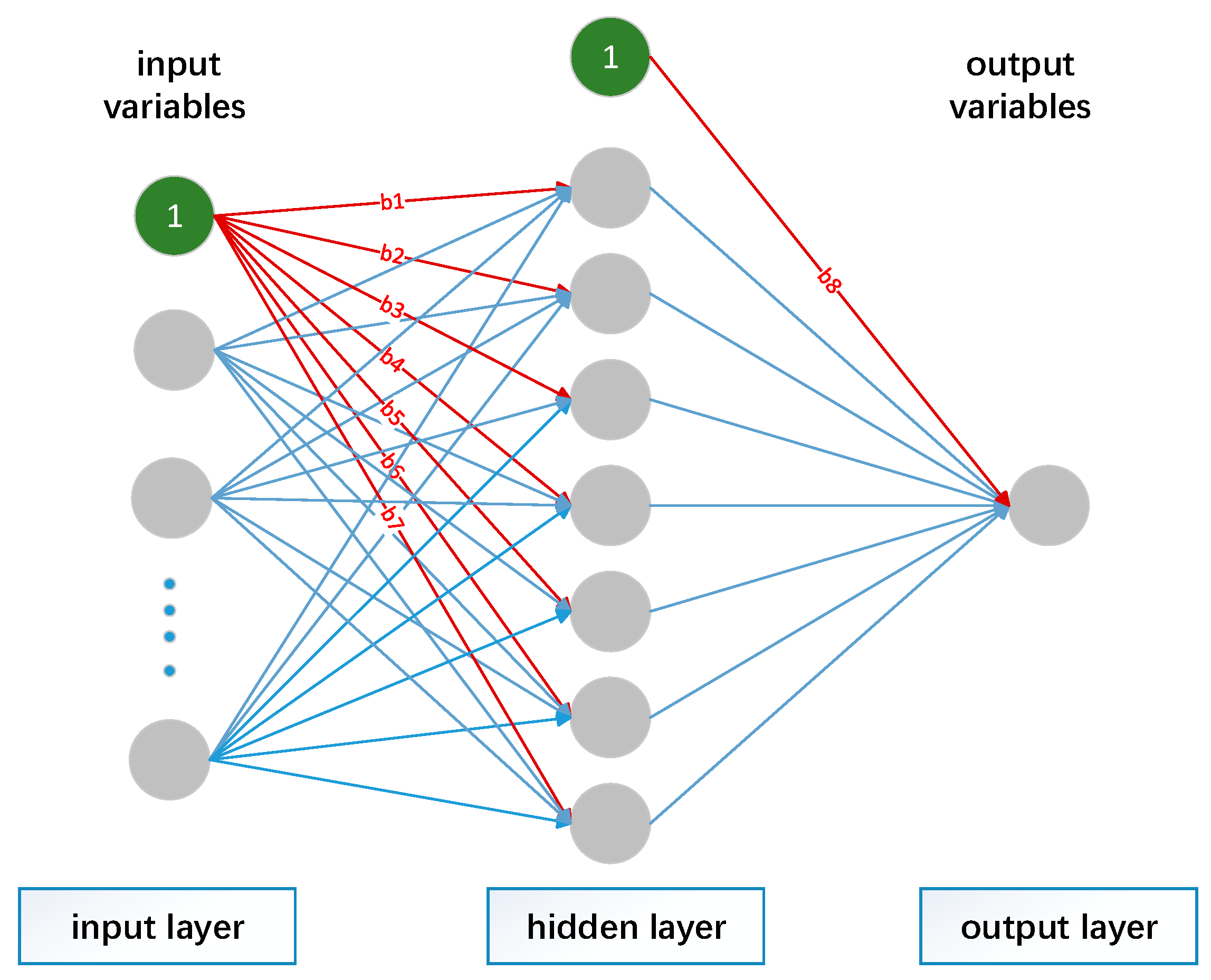
Rumelhart and McClelland proposed the back-propagation neural network (BPNN) in 1986 [27]. It is a multi-layer feedforward neural network (Figure 2 is an example) trained by the error back-propagation algorithm and is one of the most widely used artificial neural network models [28,29]. The learning rule is to use the steepest descent method and repeatedly modify weights and biases of the network through reverse iteration so that the sum of squared errors is minimized [30].

The basic training process includes two strategies. The first is forward propagation, which means that the calculation of the error output is performed from the input to the output, and the second is error back propagation, which proposes that the adjustment of weights and biases are performed from the output to the input. In the case of forwarding propagation [27], the input data affect the output node through a hidden layer and the output data are generated through non-linear transformation. If the actual output does not correspond with the predicted output, then the error is propagated backwards to eliminate as much of it as possible. Error back-propagation is used to pass the output error through the hidden nodes, layer by layer, using the error signal obtained from each layer as the basis for adjusting the weight, thus distributing the error to all nodes in each layer. By adjusting the connection strength and the bias between layers, the error is decreased along the gradient direction, and after repeated learning training, the network parameters are determined to satisfy the minimum error. The BPNN used in this study is given as follows:

$$y=f_o\left[{\displaystyle \sum }_h{w}_{oh} \times f_h\left({\displaystyle \sum }_i{w}_{hi}{x}_i+b_h\right)+b_o\right]$$

(1)

where $x_i$ is the independent input variables of training and test data, y is the output variables, $w_{hi}$ is the weight from input to hidden layer; $w_{oh}$ is the weight from hidden to output layer;$b_h$ and $b_o$ is the bias for the hidden and output layers, respectively; $f_h$ and $f_o$ are the transfer functions for hidden and output layers, respectively.

2.2.2. Genetic Algorithm

The genetic algorithm is a heuristic calculation model that simulates genetic selection and natural elimination; it has become widely known through Professor J. Holland’s work [31]. It is an efficient search algorithm for seeking optimal global solutions without any initial information [25]. The algorithm adopts the evolutionary principle of “survival of the fittest” and regards the solution set as a population. The population is continuously evolved by different kinds of genetic operations such as selection, crossover and mutation to eliminate the individuals with poor fitness and find the optimal solution that meets the requirements [32].

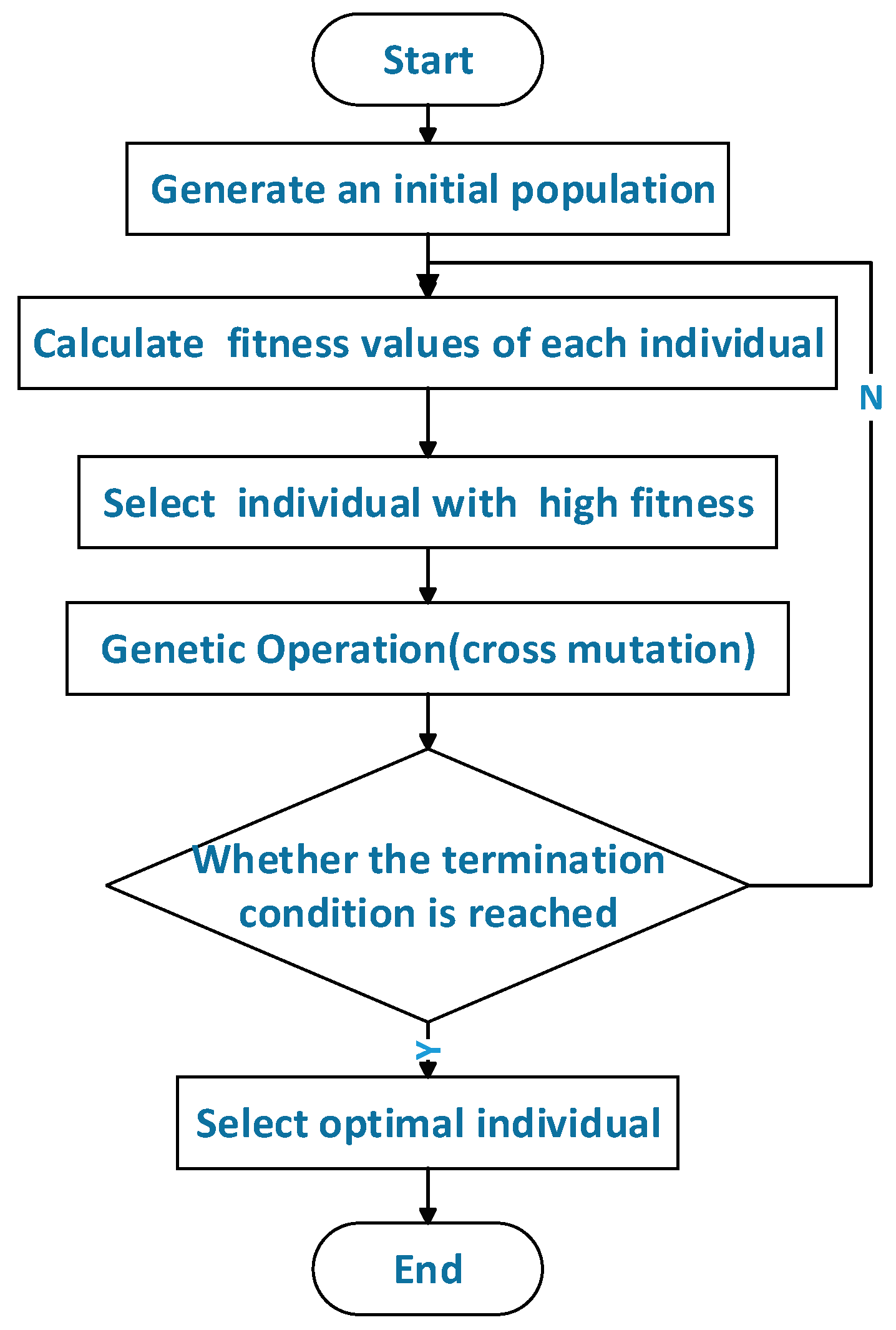
The evolutionary process of genetic algorithms is shown in Figure 3. First, some coded individuals are generated at random and grouped into an initial population. Second, each is given a fitness value calculating by the fitness function, and individuals with high fitness are selected to participate in genetic operations while others are eliminated. Furthermore, the generation consisting of individuals generated by genetic manipulation begins the next round of evolution, and the simulated evolution will not stop until the current number of generations reaches the maximum amount or the optimal individual does not improve in several consecutive generations. When the algorithm finally ends, the best-performing individual is chosen as the optimal solution or sub-optimal solution of the problem [33,34].

Genetic algorithms have strong adaptability and global optimization ability. Because they have no specific restrictions on problems or special requirements for search space, genetic algorithms are easy to combine with other algorithms. They have been widely used in some fields such as function optimization [35], neural network training [36], pattern recognition [37], and time-series prediction [38]. However, a traditional genetic algorithm can easily fall into a locally optimal solution and cannot handle complex, large-scale nonlinear constrained programming very well [25].

2.2.3. Improved Genetic Algorithm Coupled with Neural Network Model

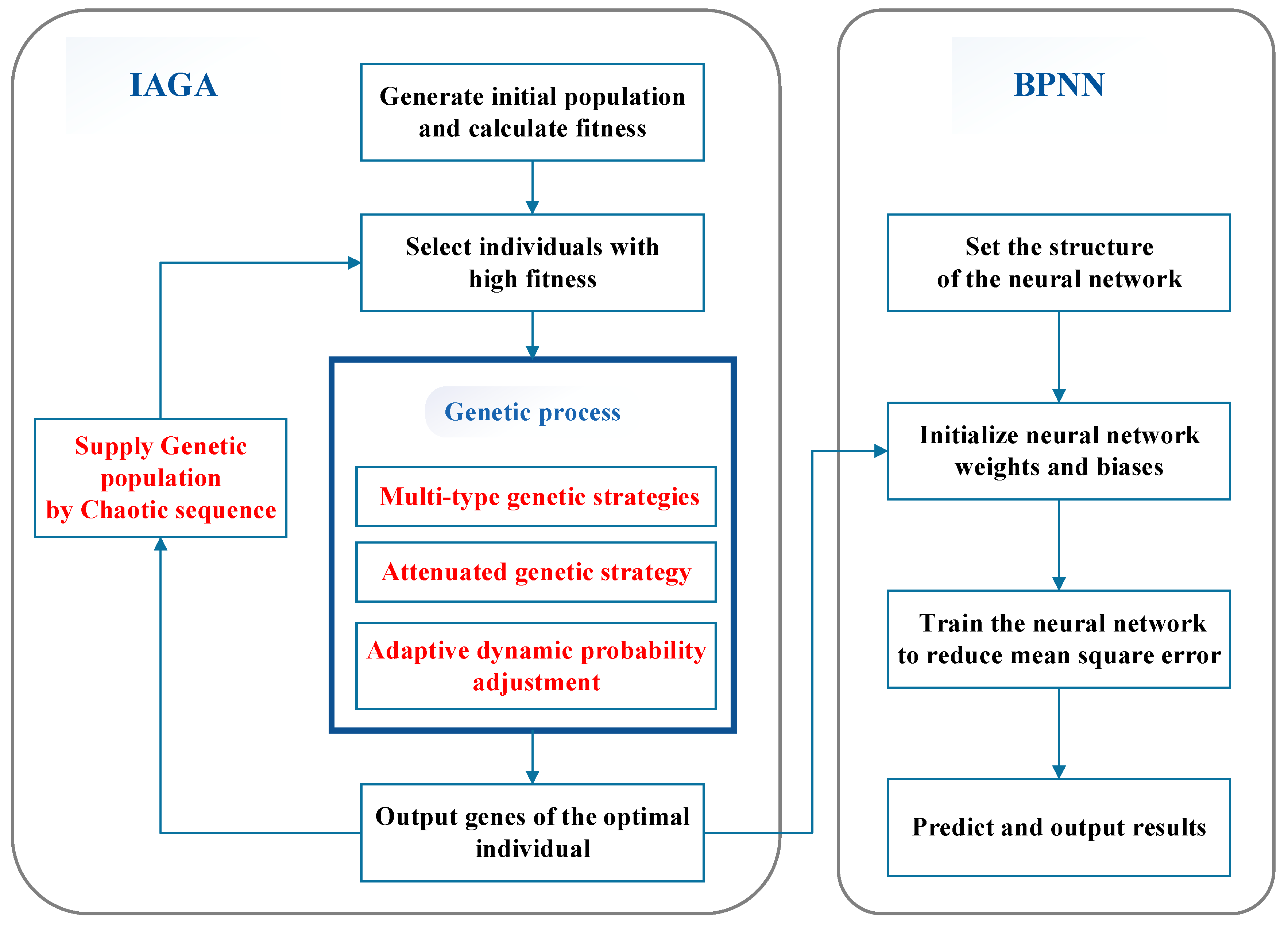
To deal with the limited optimization and local convergence problem, in this study, the supplementary population strategy, the multi-type genetic strategy, the adaptive dynamic probability adjustment and the attenuated genetic approach are used to enhance the genetic algorithm’s ability to search in the neural network. It can be seen from Figure 4 that the algorithm consists of improved adaptive genetic strategies and a back propagation neural network. By adopting an improved adaptive genetic algorithm, the optimal weight and bias are assigned to the neural network as the initial training parameter to perform the iterative training of the neural network. Then, the model stops practice and begins to predict, and it runs until the number of generations reaches the maximum amount, or the error threshold satisfies the maximum limit.

• Supply Genetic Population by a Chaotic Sequence

In a genetic algorithm, the individual number (N) of the population is always fixed. In subsequent generations, some elite individuals (N1) are kept and some (N2) are generated by genetic operations (crossover, mutation). When N1 plus N2 is less than N, the reduced number N3 (N3 = N − N1 − N2) is supplied as entirely new by a chaotic sequence. As the chaotic sequence has random and aperiodic characteristics [39], it can improve the search ability in the global space and avoid falling into the local suboptimal solution. Moreover, the initial population of the genetic algorithm can be generated by a chaotic sequence. This research adopts the logistic equation to supply the population. The basic equations are defined as follows:

$$X_{n+1} = \mu X_n\left(1-X_n\right), 0\le X_n\le 1$$

(2)

where $X_n$ is the first variable, $X_{n+1 }$ is the changed variable, $\mu$ is the control parameter, and $\mu$ = 0~4. When $\mu$ = 3.56~4, the equation completely becomes a chaotic state. The logistic equation used for initial population generation in this paper is as follows:

$$X_{i+1}=4X_i\left(1-X_i\right), 0\le X_i\le 1,i=1,2,\dots ,n$$

(3)

The supplementary population generated by the chaotic sequence can ensure that the supplemented individuals always vary around the previous generation’s optimal solution, which will improve the individual quality in the population and accelerate the overall convergence speed of the algorithm [40].

• Multi-Type Genetic Strategies

Genetics is the core operation in genetic algorithms, including genetic crossover and genetic mutation. Crossover is mainly used to exchange information between two individuals to form a generation of new individuals, and mutation is a process that increases the diversity of the population by changing the genes at a certain position with probability. Since the scale of most optimization problems is not large, the traditional crossover and mutation operations can satisfy the requirements without causing problems, such as falling into local optimal solutions. There are too many input dimensions in the water-level prediction research, which leads to each having large gene strings. Therefore, multi-point and multi-type genetics should be adopted for individuals with high complexity, meaning that multiple crossover operators are used to exchanging genes between individuals in crossover operations and multiple mutation operators are used to mutate genes on individuals in the mutation operation.

1. Multi-Type Crossover Strategy

There are multiple types of crossover operators in crossover operation. In the research, authors adopt the true arithmetic crossover and the approaching optimal solution crossover to perform the crossover operation between two individuals.

Uniform arithmetic crossover refers to having two parent individuals generate new offspring individuals through a linear transformation. The transformation formulae are expressed as follows:

$$X_A^{\text{'}}=\alpha X_B+\left(1-\alpha \right)X_A$$

(4)

$$X_B^{\text{'}}=\alpha X_A+\left(1-\alpha \right)X_B$$

(5)

where $X_A$ and $X{ }_B$ are the parent individuals before the exchange, $X_A^{\text{'}}$ and $X_B^{\text{'}}$ are the offspring after the exchange, and $\alpha$ is the proportional constant and its range is at [0,1]. However, the efficiency of general uniform arithmetic cross-optimization is too low, and it is not applicable for large and complex exchange operations. This research proposes an exchange strategy to approach the optimal solution, leading the general individual to become a better individual in the parent class. The transformation formula modified from the Nelder–Mead operator [26] is expressed as follows

$$X_A=X_{low}+{\partial }_1(X_{high}-X_{low})d,$$

(6)

$$X_B=X_{low}+{\partial }_2(X_{high}-X_{low})d$$

(7)

$$\mathrm{d}=\frac{f_{high}-f_{low}}{f_{ high}}$$

(8)

where $X_{high}$ is an individual with higher fitness, $X_{low}$ is an individual with lower fitness, $X_A$ and $X_B$ are offspring after the exchange,${\partial }_1$ and ${\partial }_2$ are proportional constants and their ranges are at [0,1], and $d$ is the search direction normalized along the fitness difference of searching for direction values. Equations (6) and (7) are nothing but the expression used for their crossover operator. The optimal solution approximation strategy introduces the continuing improvement of the individual gene patterns of the offspring, which is a good way to determine the optimization direction of the offspring individuals and avoid the possibility of local convergence of the immature individuals.

2. Multi-Type Mutation Strategy

There are multiple types of mutation operators in a mutation operation. The authors adopt a non-uniform mutation and adaptive mutation to perform the mutation operation between two individuals.

The non-uniform mutation mainly relates mutation amplitude to the number of generations, and the adaptive mutation strategy is to connect the mutation amplitude to whether it is close to the optimal solution. The transformation operation is expressed as follows [41]:

$$X_A=X+(X_{max}-X)r^{{\left(1-\frac{t}{i_m}\right)}^2}$$

(9)

$$X_B=X-\left(X-X_{min}\right)r^{{\left(1-\frac{t}{i_m}\right)}^2}$$

(10)

$$t=i$$

(11)

$$t=1-\frac{1}{f+1}$$

(12)

where $X_A$ and the $X_B$ are standard formulas used to calculate the genes of an individual after mutation, and the authors use a random variable to determine which one to choose. X is the current individual’s gene selected to participate in the mutation operation, $X_{max}$ is the upper limit of the individual’s gene domain value, $X_{min}$ is the lower limit of the individual’s gene domain value, r is a random value of 0–1, $i_m$ is the maximum number of generations, i is the current number of generations, f is the fitness value of the current operation individual, and t represents the operational variable for different mutation operators. Equation (11) is used to calculate t for non-uniform mutation, and Equation (12) is used to calculate t for the adaptive mutation. By operating alternately, the algorithm can greatly improve the efficiency of the mutation to ensure the diversity of the population.

• Adaptive Dynamic Probability Adjustment

The crossover and mutation probability of the traditional genetic algorithm are constant values. The authors adopt the adaptive genetic algorithm proposed to adjust the crossover and the mutation probability dynamically with the adaptive fitness value. The formula of adaptive dynamic probability is expressed as follows:

$$P_c=\{\begin{array}{ll}{P}_{C1},& f<f_{avg}\\ P_{c1}-\frac{\left(P_{c1}-P_{c2}\right)\left(f-f_{avg}\right)}{f_{max}-f_{avg}},& f\ge f_{avg} \end{array},$$

(13)

$$P_m=\{\begin{array}{ll}{P}_{m1},& f<f_{avg}\\ P_{m1}-\frac{\left(P_{m1}-P_{m2}\right)\left(f_{max}-f\right)}{f_{max}-f_{avg}},& f\ge f_{avg} \end{array}$$

(14)

where $P_c$ is the crossover probability, $P_m$ is the mutation probability, $f_{avg}$ represents the average fitness value of each generation,$f_{max}$ represents the maximum fitness value in the group, $f$ represents the larger adaptation value of the two individuals in Equation (13), and f represents the individual fitness value of the individual to be mutated in Equation (14). $P_{c1}$ and $P_{c2}$ represent the highest crossover probability and the lowest crossover probability. $P_{m1}$ and $P_{m2}$ represent the highest mutation probability and the lowest mutation probability.

From the perspective of the algorithm, when the mean fitness value of the entire population is stable and tends to be consistent $P_c$ and $P_m$ increase; when the fitness value differs, $P_c$ and $P_m$ decrease. Additionally, the excellent individual whose fitness value is higher than the mean value can be given a lower $P_c$ and higher $P_m$; the inferior individual with a fitness value below the mean value can be given a more top $P_c$ and higher $P_m$.

By adjusting the probability adaptively, the algorithms can not only maintain the diversity of the population but also guarantee the versatility and robustness of the algorithm.

• Attenuated Genetic Strategy

To ensure that the genetic operation can be stabilized in the process of approximating the maximum number of generations, the authors consider adopting a strategy that can gradually reduce the impact of genetic operations on the overall optimization of the process, by a multi-point and multi-type genetic coupled strategy. The authors propose an attenuated genetic strategy to decrease the number of mutated and crossed genes gradually as the number of generations increases so that the numbers of crossover and mutations can tend towards a stable value. The attenuated genetic strategy equation is expressed as follows:

$$t_c=e^{\frac{-5i}{i_m}}\times C_{max}+C_{min}$$

(15)

$$t_m=e^{\frac{-5i}{i_m}}\times M_{max}+M_{min}$$

(16)

where $t_c$ and $t_m$ represent the number of crossover and mutation on the same individual during each generation; $C_{max}$ and $M_{max}$ represent the maximum number of crossover and mutation respectively; $C_{min}$ and $M_{min}$ represent the minimum number of crossover and mutation respectively; $i_m$ is the maximum number of generations; and i is the current number of generations. It is possible to avoid the loss of excellent individuals and the degradation of the optimal search into a random search through the attenuated genetic strategy and keeping the algorithm stable.

2.2.4. Improved Genetic Algorithm Coupled with Neural Network Model

In this paper, evaluating predictive performance is the key to assessing the quality of the model and the efficiency of the optimization. This study adopted various indices to evaluate the IGA-BPNN model performance such as root mean square error (RMSE), mean squared relative error (MSRE), mean absolute error (MAE), mean absolute relative error (MARE), Nash–Sutcliffe efficiency coefficient (NSE) and Pearson correlation coefficient (R). These formulae are expressed as follows.

$$\mathrm{RMSE}= \sqrt{\frac{1}{n}{{\displaystyle \sum }}_{i = 1}^n{(y_{o,i}-y_i)}^2}$$

(17)

$$\mathrm{MSRE}=\sqrt{\frac{1}{n}{{\displaystyle \sum }}_{i =1}^n\frac{{\left(y_{o,i}-y_i\right)}^2}{y_{o,i}{}^2}}$$

(18)

$$\mathrm{MAE}=\frac{1}{n}{{\displaystyle \sum }}_{i = 1}^n\left|y_{o,i}-y_i\right|$$

(19)

$$\mathrm{MARE}=\frac{1}{n}{{\displaystyle \sum }}_{i = 1}^n\frac{\left|y_{o,i}-y_i\right|}{y_{o,i}}$$

(20)

$$\mathrm{NSE}=1-\frac{{{\displaystyle \sum }}_{i =1}^n{\left(y_{o,i }-y_i\right)}^2}{{{\displaystyle \sum }}_{i =1}^n{\left(y_{o,i}-\overline{y_o}\right)}^2}$$

(21)

$$\mathrm{R}=\frac{{{\displaystyle \sum }}_{i = 1}^n(y_{o,i} - \overline{y_o})\left(y_i - \overline{y_i}\right)}{\sqrt{{{\displaystyle \sum }}_{i = 1}^n{\left(y_{o i}-\overline{y_o}\right)}^2} \sqrt{{{\displaystyle \sum }}_{i=1}^n{\left(y_i - \overline{y_i}\right)}^2}}$$

(22)

Here, $y_{o, i}$ is the actual observation value at time i,$y_i$ is the predicted value at time i,$\overline{y_o}$ is the average of all observed values at time i, and $\overline{y_i}$ is the average of all predicted values.

RMSE provides a good measure of the goodness of fit at high flows, while MSRE provides a more balanced perspective of the goodness of fit at moderate flows. But these measures are strongly affected by catchment characteristics. MAE records the level of overall agreement between the observed and training datasets. It is a non-negative metric that has no upper bound, and for a perfect model, the result would be zero. And MARE is a relative metric which compensates for MAE which is not sensitive to the forecasting errors that occur in the low magnitudes of each dataset. But this index is not squared, the evaluation metric is less susceptible to the more significant errors that usually occur at higher scales. NSE and R, on the other hand, provide useful comparisons between studies since they are independent of the scale of data used. They are correlation measures that measure the ‘goodness of fit’ of modelled data concerning observed data.

3. Results and Discussion

3.1. Model Parameters Setting

Parameter adjustments of the genetic algorithm are still in the state of empirical adjustment, and settings need to be adjusted based on the scale of the problem and the application scenarios. After many experimental attempts for an optimal model, the training parameters of IGA are selected as shown in

Table 4. Model parameters of the improved genetic algorithm (IGA) used for the training and testing of models.

Parameter Type	IGA Parameter
Basic parameter	number of generations = 20 population size = 40
Genetic parameter	crossover probability = [0.9, 0.4] mutation probability = [0.1, 0.01] number of crossover = [50, 1] number of mutation = [20, 1]

. The minimum value for the crossover probability is 0.4, and the maximum is 0.9; the minimum value for the mutation probability is 0.01, and the maximum is 0.1; the minimum number of crossover generations is 1, and the maximum is 50; the minimum number of mutation generations is 1, and the maximum is 20. According to the initial network structure, 351 network parameters need to be trained. This means that each in the genetic algorithm has a chromosome of 351 genes. The genetic process of selection, crossover and mutation is performed on the whole population according to the fitness value, which is calculated as the mean square error. The generation will not stop until the number of generations reaches 50. The genes of the best individual in the current population are the initial weight and bias of the neural network.

The training parameters of BPNN are shown in

Table 5. Model parameters of back-propagation neural network (BPNN) used for the training and testing of models.

Parameter Type	BPNN Parameter
Study parameter	Learning rate = 0.01 momentum factor = 0.7 transfer function = $\frac{2}{1+e^{-2n}}-1$
Structure parameter	Number of input nodes = 48 (5 meteorological stations × 8 types of meteorological information per meteorological station + the water level monitored by 8 stations) number of hidden nodes = 7, number of output nodes = 1 The initial value of weight and bias = genes of best individual in IGA

. At present, there has been no common selection method for choosing the number of hidden layer nodes, learning rate and momentum rate. There is no standard for node selection while facing different types of practical problems and different kinds of data. The empirical formula is adopted to choose these parameters. M = √(n + l) + α is the formula of calculating the hidden layer nodes, n and l represent the input layer nodes and the output layer nodes, respectively, α is an adjustable random variable between 0–10. After many experimental attempts for an optimal model, the authors choose a = 0, n = 49, l = 1 and the number of the hidden layer nodes is 7. The learning rate generally values from 0.01 to 0.2, and this research uses 0.01; the momentum rate generally values from 0.6 to 0.8, here the research chooses 0.7. The selection of each parameter is a relative optimal solution obtained by multiple adjustments.

The authors used k-fold cross-validation to prevent the overfitting of neural networks. Firstly, the data is divided into 7 equal parts according to the year with normalized within [−1, 1]. Secondly, one of each is selected as the validation set, and the remaining is used as the training set. Thirdly, the second step should be repeated for 7 times so that each subset has an opportunity as a validation set. Fourthly, the result obtained from the 7 pieces of training are separately used as a prediction and evaluation model, and the average is taken as the result of the entire prediction model.

3.2. Prediction Results

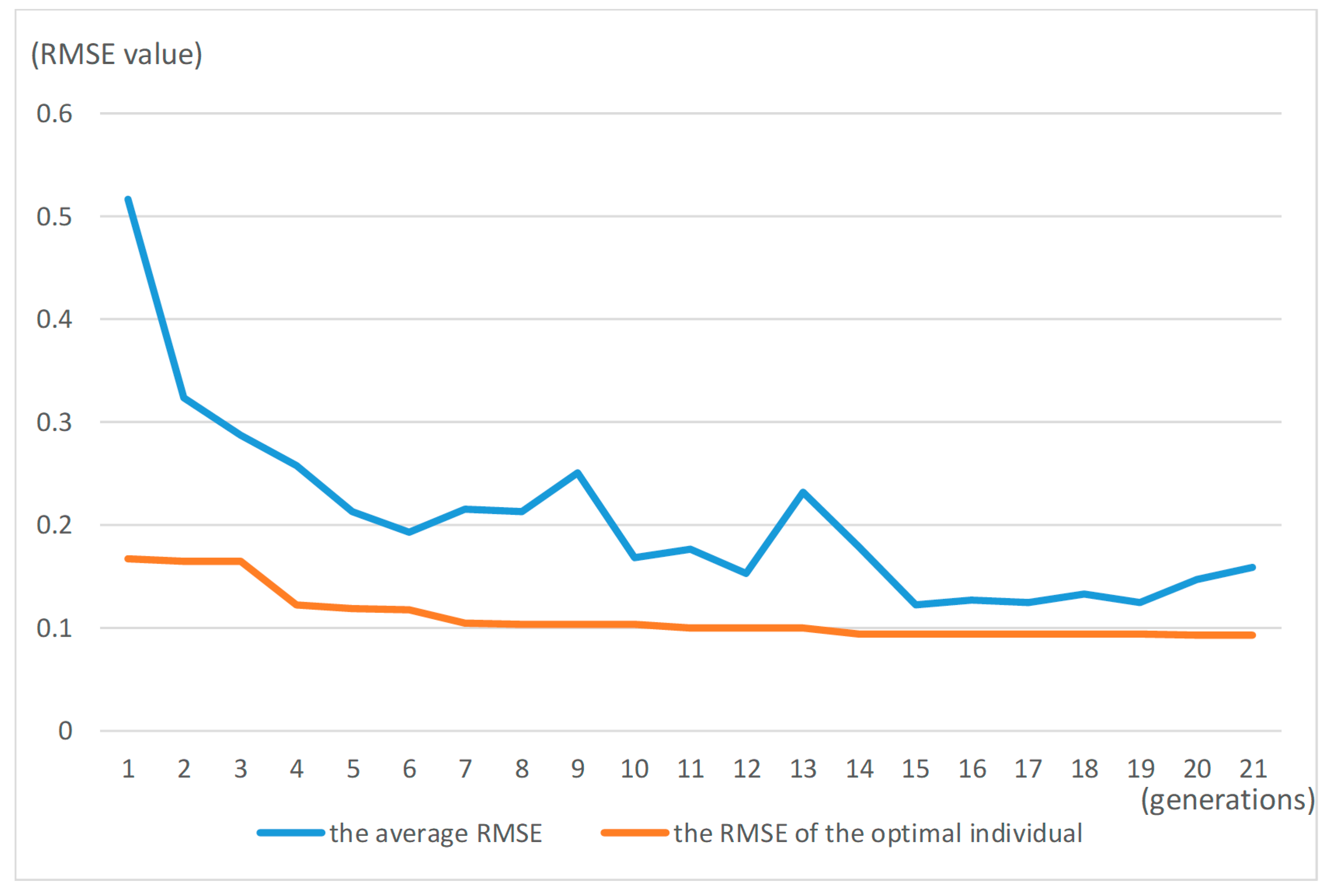
The entire training process of IGA is shown in Figure 5 and

Table 6. The RMSE value of the optimal individual and the average in the population.

Number of Generations	1	4	7	10	13	16	19	21
The RMSE value of Optimal individual	0.167	0.164	0.117	0.104	0.100	0.093	0.093	0.093
The average RMSE in population	0.516	0.287	0.193	0.251	0.152	0.122	0.135	0.147

. As can be seen from the figure, when the number of generations increases, the RMSE of the optimal individual and the average decrease gradually, which means that the fitness of the population is gradually becoming stronger through the iterative process. When the number of generations reaches a value of approximately 16, the fitness of the optimal individual has stabilized, and the change is no longer obvious. Until the end of the generation, the average RMSE value of the population is 0.1468, and the RMSE value of the optimal individual is 0.0933. Meanwhile, the gene string of the current optimal individual is the initial weight of the neural network.

Meteorological data and water-level data from 2010 to 2016 are used as training data, and 2017 data are used as the prediction data for hundreds of iteration predictions. Part of the RMSE results is shown in

Table 7. Partial RMSE values of hundreds of iteration results by using the IGA-BPNN model.

Times	1	2	3	4	5	6	7	8	9	10
RMSE	0.241	0.473	0.535	0.299	0.765	0.522	0.522	0.680	0.306	0.381
Times	11	12	13	14	15	16	17	18	19	20
RMSE	0.409	0.721	0.316	1.0988	0.0519	0.399	0.8006	0.319	0.820	0.361

. Due to the inaccuracy and randomness of the neural network, there are a few cases where the RMSE values are significant. However, in hundreds of iterations, the overall prediction accuracy of the IGA-BPNN model is at a low level, and the overall prediction accuracy is stable at approximately 0.49.

The prediction results are shown in Figure 6, which presents the fitting effect of observed and predicted data. Because of the long forecasting time, the research chose three periods to discuss the predictions in detail. The left side shows the period of less rainfall and the stable water level in March and April. The middle shows the change in water level with frequent rain and sudden flooding in September and October. The right side shows the self-regulation process of the water circulation system after heavy rain in November. These figures indicate that the IGA-BPNN model can predict water level precisely, whether the water level suddenly rises continuously or falls gradually after the heavy rain, even including daily water level monitoring. The IGA-BPNN model has good prediction accuracy for various monitoring scenarios.

3.3. Comparison of Improved Genetic Algorithm Coupling a Back-Propagation Neural Network (IGA-BPNN) with Traditional GA-BPNN and Artificial Neural Network

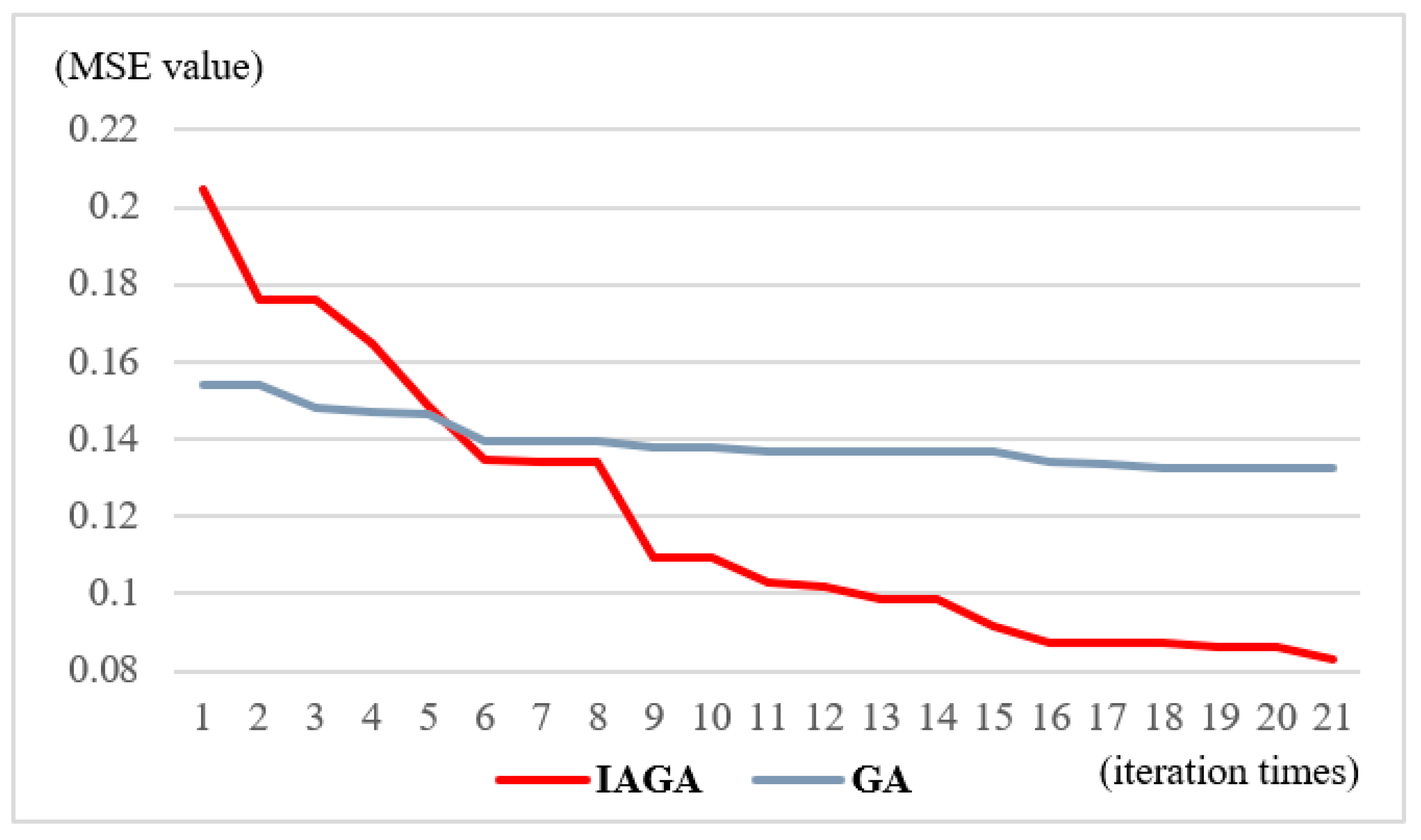
Figure 7 shows the change in the RMSE in the iterative process of the conventional GA-BPNN model and the IGA-BPNN model under the same parameters. The value of the RMSE changes from 0.154 to 0.132 in 20 generations when the research adopts the traditional GA-BPNN model. However, the IGA-BPNN model the authors proposed improves the optimization efficiency of the initial network weight significantly, as the value of the RMSE is reduced from 0.205 to 0.083. This indicates that the IGA-BPNN algorithm has higher adaptability and robustness in the water-level prediction study while using multiple input parameters.

The completeness and adequacies of three different models for 1-day-ahead forecasts are summarized in Table 6. The RMSE is a measure of the residual variance that shows the global fitness between the computed and observed water levels. Compared with GA-BPNN and the static ANN models whose RMSE values vary by approximately 0.65 m, the RMSE of the IGA-BPNN model is very good, as is evident from a low RMSE cost (<0.5 m) during both training and validation periods. The NSE is a measure of quality that evaluates the reliability of a model in the water-level-prediction application. The NSE value of the traditional ANN varies by approximately 0.7, which can only reach 0.8 even after GA optimization. However, the experimental result for the NSE of the IGA-BPNN model is about 0.9 which indicates that the improved model is of good quality. The R shows the statistical correlation between the computed and observed water levels. The results show that the deviations in the three models on the indicator are not significant and have a strong relationship, but the IGA-BPNN model still performs better. MAE and MARE measure the goodness of fit under high and medium flow respectively.

Table 8. Performance indices of water-level prediction models.

	IGA-BPNN		GA-BPNN		ANN
	Verification	Prediction	Verification	Prediction	Verification	Prediction
RMSE	0.2123	0.4722	0.3436	0.6258	0.3145	0.6432
NSE	0.9792	0.9382	0.9521	0.8233	0.9243	0.7443
R	0.9734	0.9423	0.9642	0.9257	0.9621	0.9015
MSRE	0.011	0.031	0.015	0.037	0.014	0.045
MAE	0.241	0.516	0.227	0.472	0.375	0.501
MARE	0.010	0.023	0.014	0.033	0.015	0.029

shows that IGA-BPNN performs better under high tide, but is not as good as GA-BPNN under medium flow. The result of MAE indicates that the overall agreement level between the observed and training datasets of IGA-BPNN is not good. From Table 8, it can be concluded that the IGA-BPNN model has predicted the water level with reasonable accuracy, in terms of all the evaluation indices, during the training and validation periods. Although the IGA-BPNN model does not always perform well on various evaluation indices, it is better than the others on most indices.

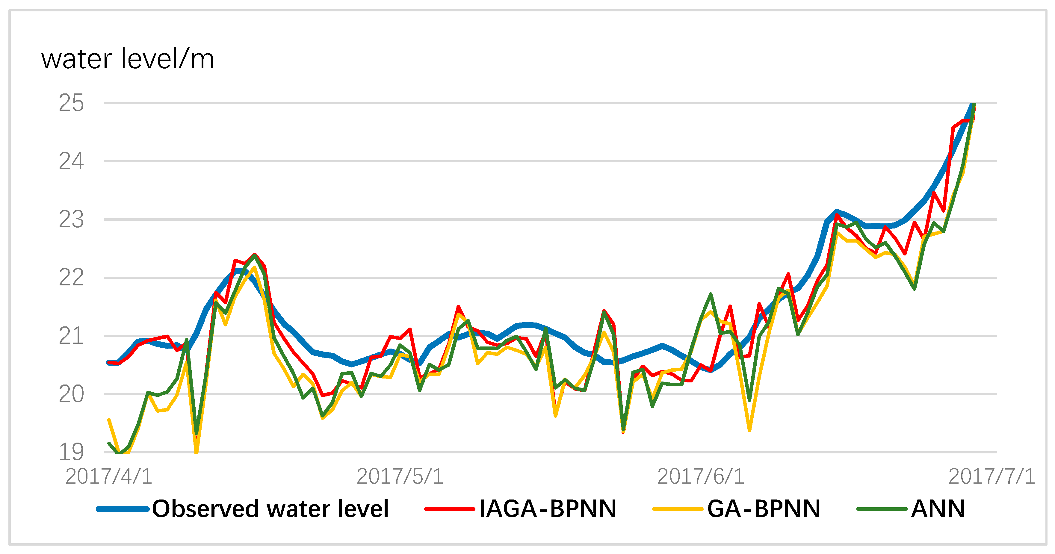
The following four figures show the comparison of the three models for water-level forecasting in 2017. Figure 8 shows the water level changes from January to March, which are in the natural regulation stage of the water cycle. The rising water level can be monitored precisely by using the IGA-BPNN model when the rainfall is low, while the traditional GA-BPNN and ANN have low prediction efficiency, which is approximately 1.5 m away from the actual water level.

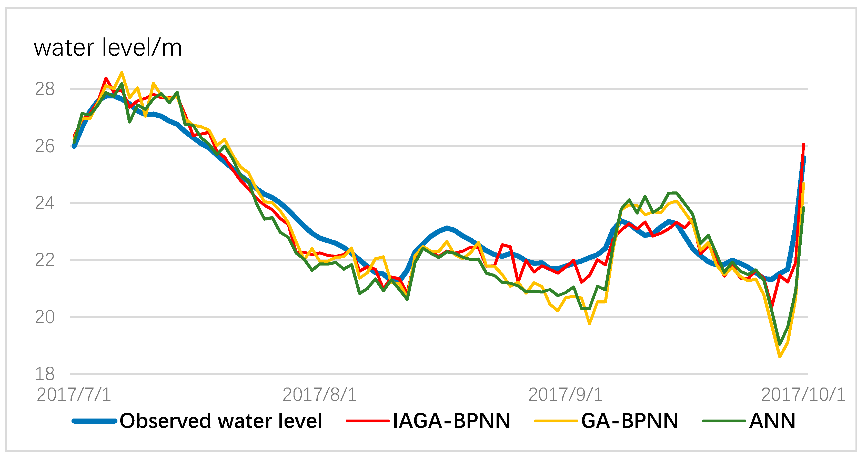
Figure 9 and Figure 10 show the water level changes when rainfall is frequent, and precipitation has a significant effect on the change in water level. Although these three models can monitor the water level dynamically and precisely, it can be observed that the IGA-BPNN model is still superior to the other models due to the actual water level curve.

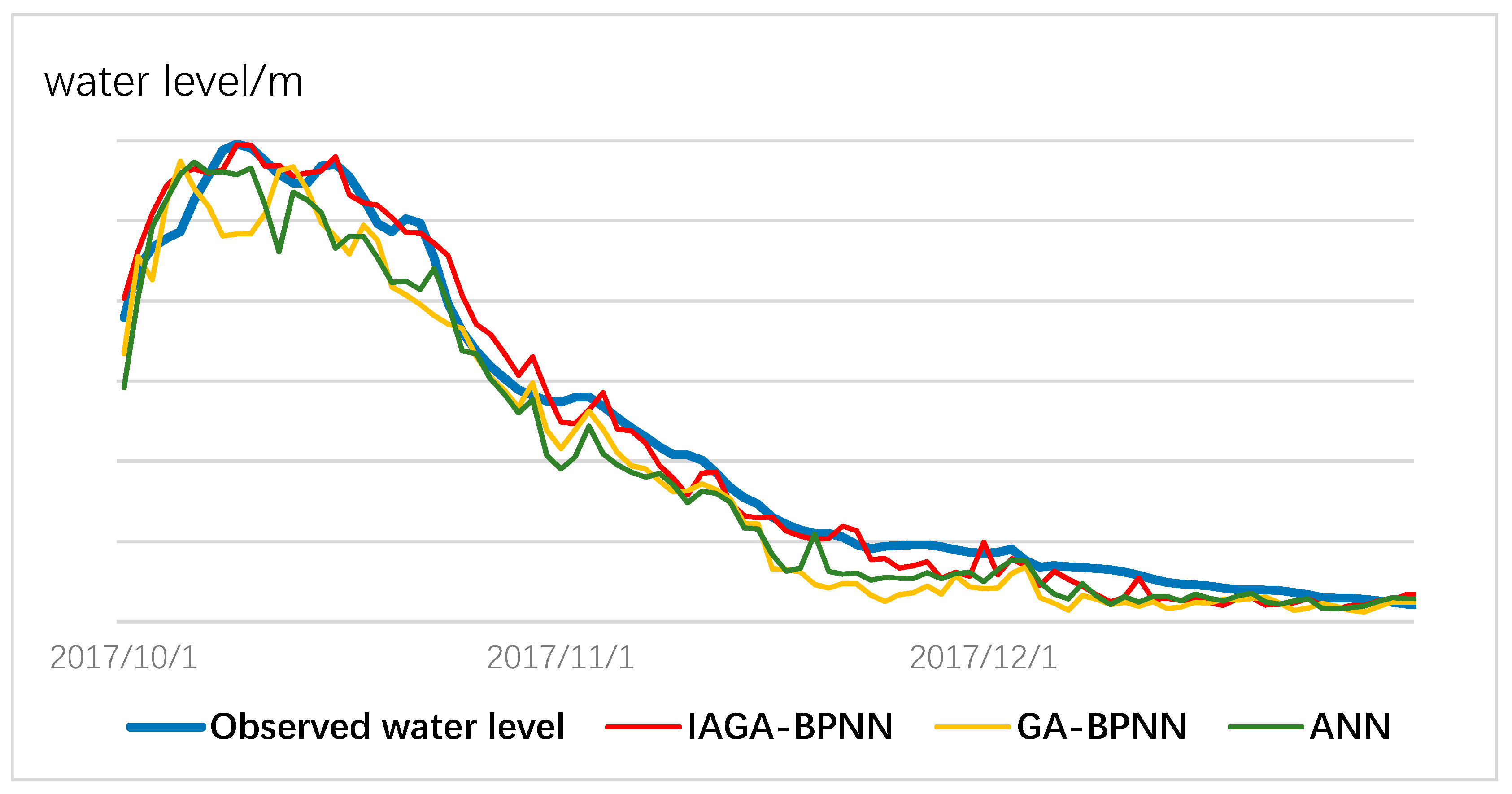
Figure 11 shows the process of water level self-regulation and recovery when the rainfall reduces gradually. It can be seen from the figure that there is flooding in mid-October, where ANN and GA-BPNN perform poorly. Conversely, the IGA-BPNN model can predict the water-level values and trends before and after flooding accurately. Compared to ANN and the traditional GA-BPNN model, IGA-BPNN can provide a higher precision for flood monitoring and warning.

As can be concluded from the experimental result, the prediction accuracy of IGA-BPNN is much higher than the other algorithms; by optimizing the network structure from the perspective of initial weight, IGA-BPNN model adopts not only genetic algorithm to obtain better initial load, but also proposes many genetic strategies to improve the problem of local optimal solutions easily caused by basic genetic algorithms while facing the large-scale iterative populations.

4. Conclusions

To address the issue of traditional GA-BPNN for accurate water-level prediction, a novel IGA-BPNN model is proposed in this study using the hybrid concepts of adaptive genetic algorithm and BPNN. The study area is located in China in the middle and lower reaches of the Han river. In this study, these researchers adopt meteorological parameters, which are easily accessible as experimental output, and select the water level observed using stations near the outlet of Han River as the prediction to verify the feasibility of the model. At the same time, the researchers test the robustness of IGA-BPNN by comparing traditional ANN and GA-BPNN models under the same training conditions. The results of this study present the following conclusions:

• The IGA-BPNN model proposed uses a variety of genetic strategies to maximize the efficiency of the genetic algorithm for neural network initial weights and biases. It can deal with the limited optimization, and local convergence is often occurring in the algorithm, while facing the complex and multi-node networks.
• Compared with the traditional ANN and GA-BPNN models, the IGA-BPNN can capture the non-linear rainfall; the water-level relationship of the studied area very well and performs better when predicting water level, regardless of frequent rain or the gentle change of water level. The IGA-BPNN model has a suitability for water-level predictions and would provide a better effect of short-term flood forecasting.

A limitation of this paper is the IGA-BPNN model only focuses on the middle and lower reaches of the Han River Basin, mainly considering the existence of artificial dams in the middle ranges. When flow rates are too large, there will be some manual intervention to adjust the flow and avoid flood events. Because the dam has a significant influence, this research chose a part of the watershed that was not affected by the dam to train and verify the prediction model. In subsequent research, the research will improve on the problems of the above algorithms and try to simulate the influence of rainfall on the water level under artificial intervention conditions.

References

- Aerts, J.; Botzen, W.; Clarke, K.; Cutter, S.; Hall, J.W.; Merz, B.; Michel-Kerjan, E.; Mysiak, J.; Surminski, S.; Kunreuther, H. Integrating human behaviour dynamics into flood disaster risk assessment. Nat. Clim. Chang. 2018, 8, 193. [Google Scholar] [CrossRef]
- Park, E.; Parker, J. A simple model for water table fluctuations in response to precipitation. J. Hydrol. 2008, 356, 344–349. [Google Scholar] [CrossRef]
- ASCE. Artificial neural networks in hydrology. I: Preliminary concepts. J. Hydrol. Eng. 2000, 5, 115–123. [Google Scholar] [CrossRef]
- Anderson, M.P.; Woessner, W.W.; Hunt, R.J. Applied Groundwater Modeling: Simulation of Flow and Advective Transport; Academic Press: Cambridge, MA, USA, 2015. [Google Scholar]
- Yoon, H.; Jun, S.-C.; Hyun, Y.; Bae, G.-O.; Lee, K.-K. A comparative study of artificial neural networks and support vector machines for predicting groundwater levels in a coastal aquifer. J. Hydrol. 2011, 396, 128–138. [Google Scholar] [CrossRef]
- Daliakopoulos, I.N.; Coulibaly, P.; Tsanis, I.K. Groundwater level forecasting using artificial neural networks. J. Hydrol. 2005, 309, 229–240. [Google Scholar] [CrossRef]
- Maier, H.R.; Dandy, G.C. Neural networks for the prediction and forecasting of water resources variables: A review of modelling issues and applications. Environ. Model. Softw. 2000, 15, 101–124. [Google Scholar] [CrossRef]
- Nayak, P.C.; Rao, Y.S.; Sudheer, K. Groundwater level forecasting in a shallow aquifer using artificial neural network approach. Water Resour. Manag. 2006, 20, 77–90. [Google Scholar] [CrossRef]
- Bustami, R.; Bessaih, N.; Bong, C.; Suhaili, S. Artificial neural network for precipitation and water level predictions of Bedup River. IAENG Int. J. Comput. Sci. 2007, 34, 228–233. [Google Scholar]
- Adamowski, J.; Chan, H.F. A wavelet neural network conjunction model for groundwater level forecasting. J. Hydrol. 2011, 407, 28–40. [Google Scholar] [CrossRef]
- Piasecki, A.; Jurasz, J.; Skowron, R. Forecasting surface water level fluctuations of lake Serwy (Northeastern Poland) by artificial neural networks and multiple linear regression. J. Environ. Eng. Landsc. Manag. 2017, 25, 379–388. [Google Scholar] [CrossRef]
- Zhong, C.; Jiang, Z.; Chu, X.; Guo, T.; Wen, Q. Water level forecasting using a hybrid algorithm of artificial neural networks and local Kalman filtering. J. Eng. Marit. Environ. 2019, 233, 174–185. [Google Scholar] [CrossRef]
- Wang, Y.; Tabari, H.; Xu, Y.; Xu, Y.; Wang, Q. Unraveling the role of human activities and climate variability in water level changes in the Taihu plain using artificial neural network. Water 2019, 11, 720. [Google Scholar] [CrossRef]
- Faruk, D.Ö. A hybrid neural network and ARIMA model for water quality time series prediction. Eng. Appl. Artif. Intell. 2010, 23, 586–594. [Google Scholar] [CrossRef]
- Zhang, G.P. Time series forecasting using a hybrid ARIMA and neural network model. Neurocomputing 2003, 50, 159–175. [Google Scholar] [CrossRef]
- Bazartseren, B.; Hildebrandt, G.; Holz, K.-P. Short-term water level prediction using neural networks and neuro-fuzzy approach. Neurocomputing 2003, 55, 439–450. [Google Scholar] [CrossRef]
- Kuremoto, T.; Kimura, S.; Kobayashi, K.; Obayashi, M. Time series forecasting using a deep belief network with restricted Boltzmann machines. Neurocomputing 2014, 137, 47–56. [Google Scholar] [CrossRef]
- Wang, L.; Zeng, Y.; Chen, T. Back propagation neural network with adaptive differential evolution algorithm for time series forecasting. Expert Syst. Appl. 2015, 42, 855–863. [Google Scholar] [CrossRef]
- Khan, A.U.; Bandopadhyaya, T.K.; Sharma, S. Genetic algorithm based backpropagation neural network performs better than backpropagation neural network in stock rates prediction. Int. J. Comput. Sci. Netw. Secur. 2008, 8, 162–166. [Google Scholar]
- Kisi, O.; Alizamir, M.; Zounemat-Kermani, M. Modeling groundwater fluctuations by three different evolutionary neural network techniques using hydroclimatic data. Nat. Hazards 2017, 87, 367–381. [Google Scholar] [CrossRef]
- Fonseca, C.M.; Fleming, P.J. An overview of evolutionary algorithms in multiobjective optimization. Evol. Comput. 1995, 3, 1–16. [Google Scholar] [CrossRef]
- Zitzler, E.; Thiele, L. Multiobjective evolutionary algorithms: A comparative case study and the strength Pareto approach. IEEE Trans. Evol. Comput. 1999, 3, 257–271. [Google Scholar] [CrossRef]
- Sedki, A.; Ouazar, D.; El Mazoudi, E. Evolving neural network using real coded genetic algorithm for daily rainfall–runoff forecasting. Expert Syst. Appl. 2009, 36, 4523–4527. [Google Scholar] [CrossRef]
- Dash, N.B.; Panda, S.N.; Remesan, R.; Sahoo, N. Hybrid neural modeling for groundwater level prediction. Neural Comput. Appl. 2010, 19, 1251–1263. [Google Scholar] [CrossRef]
- Sivanandam, S.; Deepa, S. Genetic algorithm optimization problems. In Introduction to Genetic Algorithms; Springer: Berlin/Heidelberg, Germany, 2008; pp. 165–209. [Google Scholar]
- Singh, D.; Agrawal, S. Self organizing migrating algorithm with nelder mead crossover and log-logistic mutation for large scale optimization. In Computational Intelligence for Big Data Analysis; Springer International Publishing: Cham, Switzerland, 2015; pp. 143–164. [Google Scholar]
- Rumelhart, D.E.; Hinton, G.E.; Williams, R.J. Learning representations by back-propagating errors. Nature. 1986, 323, 533–536. [Google Scholar] [CrossRef]
- Chen, F.-C. Back-propagation neural networks for nonlinear self-tuning adaptive control. IEEE Control Syst. Mag. 1990, 10, 44–48. [Google Scholar] [CrossRef]
- Goh, A.T. Back-propagation neural networks for modeling complex systems. Artif. Intell. Eng. 1995, 9, 143–151. [Google Scholar] [CrossRef]
- Buscema, M. Back propagation neural networks. Subst. Use Misuse 1998, 33, 233–270. [Google Scholar] [CrossRef]
- Holland, J. Adaptation in Natural and Artificial Systems: An Introductory Analysis with Application to Biology; University of Michigan Press: Ann Arbor, MI, USA, 1975. [Google Scholar]
- Hassan, R.; Cohanim, B.; De Weck, O.; Venter, G. A comparison of particle swarm optimization and the genetic algorithm. In Proceedings of the 46th AIAA/ASME/ASCE/AHS/ASC structures, structural dynamics and materials conference, Austin, TX, USA, 18–21 April 2005; p. 1897. [Google Scholar]
- Kuo, J.-T.; Wang, Y.-Y.; Lung, W.-S. A hybrid neural–genetic algorithm for reservoir water quality management. Water Res. 2006, 40, 1367–1376. [Google Scholar] [CrossRef]
- Wang, W.; Ding, J. Wavelet network model and its application to the prediction of hydrology. Nat. Sci. 2003, 1, 67–71. [Google Scholar]
- Niaona, Z.; Dejiang, Z.; Yong, F. The optimal design of terminal sliding controller for flexible manipulators based on chaotic genetic algorithm. Control Theory Appl. 2008, 25, 451–455. [Google Scholar]
- Xian, Z.; Wu, H.; Siqing, S.; Shaoquan, Z. Application of genetic algorithm-neural network for the correction of bad data in power system. In Proceedings of the 2011 International Conference on Electronics, Communications and Control (ICECC), Ningbo, China, 9–11 September 2011; pp. 1894–1897. [Google Scholar]
- Kim, H.-D.; Park, C.-H.; Yang, H.-C.; Sim, K.-B. Genetic algorithm based feature selection method development for pattern recognition. In Proceedings of the 2006 SICE-ICASE International Joint Conference, Busan, Korea, 18–21 October 2006; pp. 1020–1025. [Google Scholar]
- Li, P.; Tan, Z.; Yan, L.; Deng, K. Time series prediction of mining subsidence based on genetic algorithm neural network. In Proceedings of the 2011 International Symposium on Computer Science and Society, London, UK, 26–28 September 2011; pp. 83–86. [Google Scholar]
- Gao, C.; Wang, B.; Zhou, C.J.; Zhang, Q. Multiple sequence alignment based on combining genetic algorithm with chaotic sequences. Genet. Mol. Res. 2016, 15, 1–10. [Google Scholar] [CrossRef] [PubMed]
- Wu, C.L.; Chau, K.-W. A flood forecasting neural network model with genetic algorithm. Intjenvironpollut 2006, 28, 261–273. [Google Scholar] [CrossRef]
- Michalewicz, Z.; Janikow, C.Z.; Krawczyk, J.B. A modified genetic algorithm for optimal-control problems. Comput. Math. Appl. 1992, 23, 83–94. [Google Scholar] [CrossRef]
Figure 1.
The location of meteorological stations and water-level stations in the Han River basin.
Figure 2.
Basic structure of back-propagation neural network.
Figure 3.
Necessary iterative steps of the traditional genetic algorithm.
Figure 4.
Basic execution process of the improved genetic algorithm coupling a back-propagation neural network (IGA-BPNN) model and 4 types of genetic improvement strategies.
Figure 5.
The root mean square error (RMSE) curve of the optimal individual and the average in the population.
Figure 6.
The water level results predicted by the IGA-BPNN and the comparison results between the predicted and observed data of partial periods.
Figure 7.
The comparison result of iterative efficiency using IGA and GA.
Figure 8.
Comparison results for the three models for water-level prediction from January to March 2017.
Figure 9.
Comparison results for the three models for water-level prediction from April to June 2017.
Figure 10.
Comparison results for the three models for water-level prediction from July to September 2017.
Figure 11.
Comparison results for the three models for water-level prediction from October to December 2017.