Using Bayesian Networks to Assess Effectiveness of Phosphorus Abatement Measures under the Water Framework Directive


1
Faculty of Humanities, Charles University, 158 00 Prague 5, Czech Republic
2
Faculty of Social and Economic Studies, Jan Evangelista Purkyně University in Ústí nad Labem, 400 96 Ústí nad Labem, Czech Republic
*
Author to whom correspondence should be addressed.
Water 2019, 11(9), 1791; https://doi.org/10.3390/w11091791
Submission received: 23 July 2019
/
Revised: 16 August 2019
/
Accepted: 26 August 2019
/
Published: 28 August 2019
(This article belongs to the Section Water Quality and Contamination)
Abstract
:The EU Water Framework Directive requires all water bodies within the EU member states to achieve a “good status”. Many economic assessments assume the “good status” is achieved using selected measures and evaluate only associated costs and benefits. In this paper, Bayesian networks are used to test this assumption by evaluating whether the “good status” can be achieved with the selected abatement measures. Unlike in deterministic analysis, Bayesian networks allow effectiveness of measures of the same type to vary, which adds credibility to the analysis by increasing its robustness. The approach was tested on Stanovice reservoir in Czechia using a set of 244 previously designed measures. The results show the target will be met with a probability of 72.4% using the most cost-efficient measures. Based on the results, improvements to the measure selection process are suggested.
1. Introduction
There is only little doubt that eutrophication causes accelerated growth of harmful algal blooms, whether the nutrient enrichment comes from sewage or agricultural runoff [1,2,3]. In a reaction to increasing concerns about water quality, the European Commission introduced Directive 2000/60/EC of the European Parliament and of the Council of 23 October 2000 establishing a framework for Community action in the field of water policy ([4], abbreviated to WFD). The directive introduced a “good status” and required all water bodies to achieve it by 2015. The “good status” ensures that the water body departs only slightly from the biological community and hydrological and chemical characteristics that would be expected under conditions of minimal anthropogenic impact, as described in Annex V to the WFD. The “good status” consists of ecological status and chemical status in case of natural bodies or ecological potential and chemical status in heavily modified water bodies – each based on multiple criteria. The WFD applies the “one-out, all-out” principle in assessing the “good status”. Failing to satisfy just one of the indicators means the “good status” is not achieved. For this reason, the majority of European water bodies had not met the required standard by 2015. Based on [5], only 40% of surface water bodies were in good ecological status or potential and only 38% of the bodies were in good chemical status. Excessive phosphorus inflow and eutrophication belong among the key reasons for not achieving the “good status”, especially in the case of water reservoirs. However, failing to achieve the “good status” may not mean violating the regulation. Water bodies may apply for an exemption if, e.g., costs of achieving the “good status” exceed generated benefits (the WFD does not state how large the gap needs to be). The application has to be supported by economic analysis of costs and benefits, which will inevitably be spatially distributed as discussed by [6,7]. If the exemption is approved, the deadline can be extended to 2021/2027 or a lower target can be set. The requirement of achieving the “good status” has a significant impact on management of water resources in the form of pollution modelling and planning of measures.
Numerous methodologies have been created in European countries to tackle cost proportionality of achieving the “good status” [8,9,10,11,12,13,14]. These approaches use cost-benefit analysis (CBA) or criteria to assess cost proportionality of measure implementation. Martin-Ortega et al. [15] use hydro-chemical models to simulate effectiveness of phosphorus mitigation measures, but most of the time effectiveness of measures is simply assumed. Designed measures are expected to reduce exactly the desired amount of the problematic substance. Robustness is often tested by sensitivity analysis of costs and benefits but testing of the abatement effect is rather scarce (e.g., Berbel et al. [16] perform an analysis of uncertainty for both costs and efficiency of water-saving measures). Effectiveness of measures of a certain type is predetermined and constant, regardless of local conditions. This can hardly be true as not all measures have identical parameters and they are implemented under heterogeneous conditions. This means the reduction target might not be met and consequently, estimated benefits may be unrealistically high.
This paper aims to deal with uncertainty of measure effectiveness in the context of a proportionality analysis, which compares costs of measure implementation with benefits generated by achieving the “good status”. This is important under the WFD, because it allows a water body to not achieve the “good status” if the associated costs significantly outweigh the generated benefits. The approach to the proportionality analysis under the WFD is not unified, which is discussed, e.g., by [7].
However, it is inappropriate to compare costs with benefits without knowing how likely the “good status” will be achieved with the selected measures. A deterministic analysis selects measures that are expected to meet the target without any further testing, possibly using ranges to account for uncertainty. The statistical approach of the Bayesian networks makes all the approaches based on CBA more accurate by providing such information. The idea is to apply the Bayesian networks prior to the economic analysis to determine whether the “good status” can be achieved using the selected measures. Unlike a standard CBA, Bayesian analysis does not automatically assume that the target will be met. Instead, Bayesian analysis reports the probability of achieving the target, which should precede the CBA. Knowledge of this probability is important as the generated benefits would undoubtedly be lower if the target was not met. This approach improves water quality management when it comes to measure implementation and may be used to make the CBA more precise. The main objective of this paper is to describe the Bayesian networks approach, which is demonstrated on a case study of Stanovice water reservoir.
Heckerman [17] describes a Bayesian network as “a graphical model for probabilistic relationships among a set of variables”. These are an integral part of influence diagrams, which also include utility nodes and decision nodes. He provides rigorous derivation of the approach, including distribution analysis, inference, or a method for learning structure and parameters.
The Bayesian view of probability differs significantly from the classical approach. Heckerman [18] describes the frequentist approach as analyzing the probability “P” of seeing specific data given a hypothesis—P(D|H), where “D” stands for data and “H” for hypothesis. On the contrary, the Bayesian approach considers the probability of a hypothesis being true given the data—P(H|D). While classical probability is a true state of the world and is set, Bayesian probability is much closer to one’s degree of belief. However, it still satisfies the rules of probability and is not necessarily subjective. As shown by [19], the Bayesian approach based on empirical data is the same as the frequentist approach, which uses pooling of available data, and Bayesian analysis based on uninformative prior distribution is similar to frequentist analysis based on observed data. Only when expert opinion is used to form a prior, Bayesian analysis may be viewed as subjective.
Heckerman [17] shows that we can learn about parameters after defining variables, assigning priors and using Bayes’ rule (1), which updates beliefs about the parameters of given data.
All the terms in the equation above also depend on our belief. P(H|belief) is called a prior, P(D|H, belief) a likelihood and P(H|D, belief) a posterior.
Bayesian networks are used heavily in different fields, e.g., software assistance [20], medical diagnosis [21] or manufacturing control [22]. Bayesian networks are becoming increasingly popular in environmental sciences partly because of the introduction of the WFD. Hamilton et al. [23] use them to confirm the relationship between nutrient levels and algal bloom initiation. They find that the probability goes up when nutrient inflows from land runoff and point sources increase. In water management, Bayesian networks can also be used to implement uncertainty about effectiveness of measures. Probability of achieving the selected target is obtained as a result of this analysis. Outputs of such an analysis are more robust and can be used by policy makers. Compared to a deterministic analysis, the results are probabilistic and do not provide a simple yes/no answer. Nevertheless, knowing whether the “good status” can be achieved with the selected measures is crucial in proportionality analysis.
Ames et al. [24] provide a guideline for authors who plan to use Bayesian analysis in watershed management. They focus on defining the problem as a graphical structure, which includes identification of management endpoints, alternatives, data sources, variables and their discretization. They show how to build conditional probability tables (based on observed data, a simulation model or expert judgement) and demonstrate the approach on phosphorus management in the East Canyon watershed in Utah.
Different authors use networks of various complexity, ranging from a very simple model used by [25] to a complex network consisting of 35 nodes used by [26]. Some papers focus solely on satisfying a given limit, e.g., [24], while others model sustainability of several coastal lake catchment systems [27]. Studies also differ in input data as Bayesian networks are not limited to empirical inputs. These are prevalent, but they are often complemented by use of expert judgement, e.g., [28], regression or process-based models, e.g., [26], or dynamic models such as MyLake [29]. Collected data are discretized in most of the papers, but [30] develop a regression-oriented Tree Augmented Naive Bayes, which can work with continuous variables and allows for dependence among explanatory variables. The authors present risk maps of exceeding the nitrogen limit. Other examples of Bayesian network application in water management can be found in, e.g., [31,32,33]. The paper is structured as follows. The next section introduces the area and local conditions of Stanovice reservoir. Other parts of Section 2 demonstrate the methodological approach used and its application to the Stanovice water reservoir, where phosphorus abatement measures are to be implemented to satisfy the WFD requirement of the “good status”. The results are presented in a following section, and discussion and conclusions follow.
2. Materials and Methods
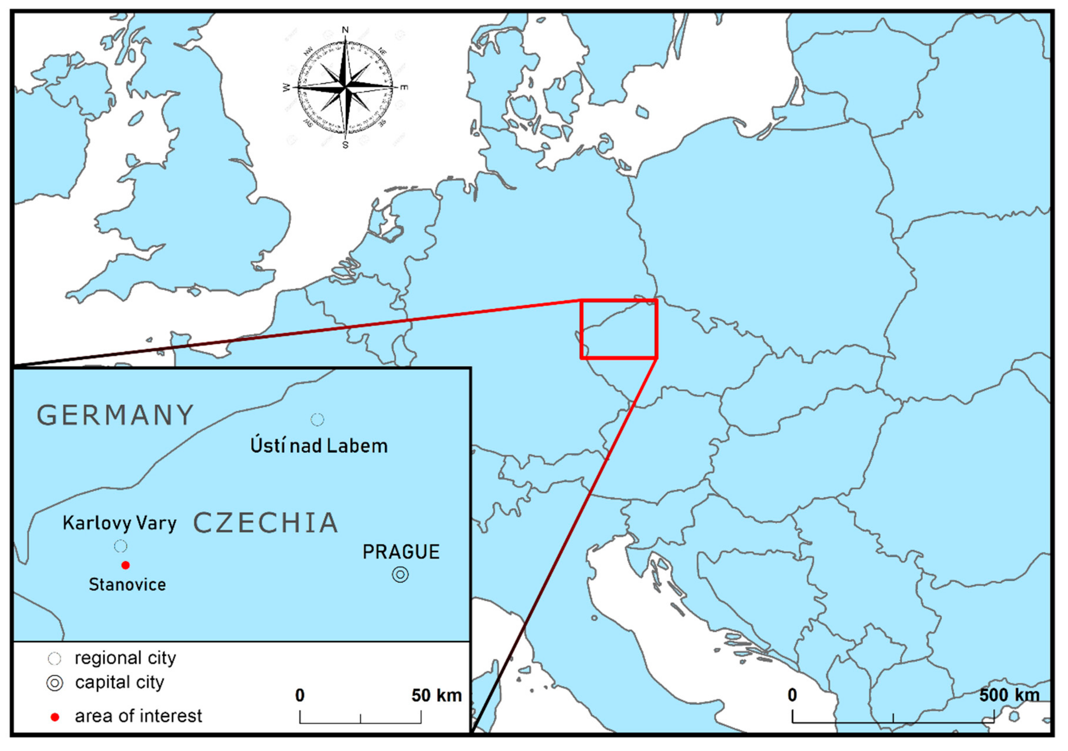
Stanovice reservoir is situated in the Czech Republic next to the city of Karlovy Vary in North-West Bohemia (Figure 1). The catchment area covers 92 km2. The main purpose of the Stanovice reservoir is to supply the Karlovy Vary area with drinking water. Its minor functions include fishery, flood protection and electricity generation.
Based on [34], Stanovice fails to achieve the “good status” mainly because of anthropogenic effects in the surrounding area such as agriculture and population. The whole area suffers from cyanobacterial growths in summer as a result of excessive inflows of dissolved phosphorus. Based on an analysis of [35,36], the main sources of phosphorus are wastewater, especially from small villages without wastewater treatment, and agriculture due to water erosion from fields into watercourses. This fact lowers the recreational benefits and makes the drinking water treatment more expensive (although the water body does not achieve the “good status”, it can still be used as a water reservoir. The “good status” depends on chemical status and ecological potential defined in the WFD, which are not directly related to suitability for drinking. The water is drinkable after receiving proper treatment). Point sources and diffuse sources contribute evenly to the total inflows. T. G. Masaryk Water Research Institute estimated that 60–200 kg of dissolved phosphorus needs to be reduced annually to achieve the “good status”. The upper bound was used in the analysis.
Dostál & Krása and Ansorge & Drozd [35,36] identified several groups of measures on both point sources (construction and renovation of wastewater treatment plants, sewerage systems, dead-end and accumulation cesspits, retention wetlands, biological reservoirs, domestic wastewater treatment plants, intensification of the treatment process in wastewater treatment plants) and agricultural land (e.g., broad-base terraces, building ditches, grassing, afforestation, contour farming, leaving crop residue, wetland establishment) as viable options for reducing phosphorus inflows. Within these groups, many individual measures of the same type were identified and specific locations in the Stanovice catchment were found where these measures can be implemented. However, not all the measures are necessary to improve the reservoir status. Therefore, an economic approach was used to identify the most cost-efficient ones [7]. The five most common and theoretically the most efficient groups of agricultural measures were selected and used together with the measures on point sources in the analysis (broad-base terraces (BBT), vegetated filter strips (VFS), changes in crop rotation (CCR), leaving crop residue (LCR), no-tillage methods (NTM), (re)construction of wastewater treatment plants (WWTP) and sewerage systems (SW), cleaning of biological ponds). In total, that represents a pool of 244 specific measures that have a potential to reduce 344.6 kg of dissolved phosphorus a year. However, that is more than the required threshold of 200 kg a year. Annualized costs and phosphorus amounts reduced were also estimated for each specific measure by [35,36], and the measures were ranked based on their cost-effectiveness (costs per kg reduced). To assess economic efficiency, the authors use a dynamic cost-effectiveness analysis [37]. Table 1 presents an overview of the selection process. The measure types in italics were included in the final analysis.
The desired threshold of 200 kg a year can be reached by implementation of 99 measures with the total annualized costs of EUR 43,233. Five of the selected measures are on point sources (especially construction of WWTPs). Despite the small number of measures on point sources, they contribute 62% to the total reduction.
2.1. Methodology
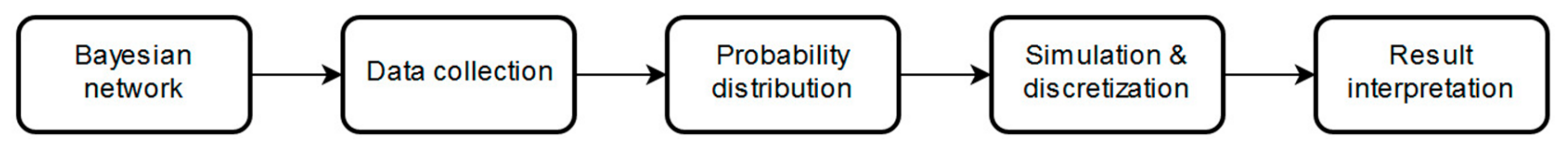
The approach used in this paper is illustrated in Figure 2. The analysis begins with the construction of a Bayesian network. It is important to decide what variables are used as inputs to the model and to define causalities among them. This is followed by data collection. Most importantly, it is necessary to determine how effective the groups of measures are in reality. Therefore, it is necessary to obtain information about what percentage of the existing amount of phosphorus a given measure can reduce. Such information may come from empirical data if a similar measure has already been used elsewhere or from literature if such a measure has been tested under laboratory/field conditions. Since no two measures in the same group will be completely identical, the resulting effectiveness will differ for most of the individual measures. Therefore, one cannot use a single number to determine the effectiveness of a group of measures and it is more appropriate to use the collected data to estimate probability distributions for each group of measures instead. If the dataset is large enough, it is possible to skip this step and go straight to discretization. Ames et al. [24] use historical records to form probability distributions of streamflow and phosphorus concentration. However, this requires hundreds of observations, which were not available for our case study. Alternatively, it is possible to use the data described above to estimate a probability distribution for each group of measures and simulate a large number of values, which are then discretized into intervals (e.g., [33] use simulation models to learn about conditional probabilities and dependencies). This method is not as demanding on data and only dozens of observations are needed. It is more preferable to use a small number of intervals, which may represent a degree to which a given group of measures reduces the present amount of phosphorus. Yu et al. [38] concluded that more than two intervals should be used. Based on that, 4 intervals of levels of phosphorus reduction effectiveness (minimum, low, medium, high) were defined. Based on the number of observations in each interval, a probability of measure effectiveness falling into that specific interval is determined using (2) for each group of measures.
The resulting probabilities enter the previously designed Bayesian network. Netica software (available at https://www.norsys.com/download.html) is then used to simulate the case study. It is a tool for working with belief networks and it allows definition of relationships between variables as probabilities. Using algorithms and known probabilities, Netica estimates the probabilities that are unknown. In this case, the software also knows the maximum amount of phosphorus that a given group of measures can reduce from Table 1. Therefore, it is possible to define each interval in terms of kilograms reduced. Using this information, probabilities of all intervals and dependencies among variables, Netica simulates many different scenarios and gives an outcome in terms of a probability that a scenario reduces at least the desired amount of phosphorus. The final step is to interpret the results, which is not trivial due to their probabilistic nature. It is important to consider how close to 100% one wants to get. Overall, the analysis is quite straightforward as no attempt was made to model the whole ecosystem and all indicators of the “good status”, but only reduction of the phosphorus from the identified load pathways was considered.
2.2. Data
As stated above, a considerable number of observations is required, because the analysis estimates a probability of achieving a certain goal based on information about previously implemented measures. However, no data about agricultural measures that would compare the situation prior to and after measure implementation are available in the Czech Republic. Therefore, results of empirical experiments from literature were used to collect as many observations as possible to estimate the probability distributions. See Supplementary Materials for more details. Despite using the available literature, our samples for changes in crop rotation and broad-base terraces remain unsatisfactory and are not included in the analysis. As for WWTPs, municipalities where a WWTP had recently been built or intensified were addressed. Although the municipalities often differ in size from the ones where the measures will be applied, it still gives a decent idea about their effectiveness and whether they comply with their respective limits. Stricter limits are enforced in larger cities, but what is important for the analysis is how the real effectiveness compares with the concentration limits for which a given WWTP was designed. A similar approach was used for WWTP and sewerage system construction. Data on recently built WWTPs (last 6 years) were collected to get a satisfactory dataset (the sample consists of more than 100 sewerage and WWTP construction projects, including renovation and intensification). Unfortunately, the last measure on point sources (biological ponds) is quite unique in the Czech Republic and no data about its effectiveness exist. In such cases, expert judgement may be used to form a triangular distribution as suggested by [28], or a uniform distribution can be used if the parameters cannot be estimated. However, the authors want to keep this case study as empirical as possible and this measure was discarded. Therefore, only five of the measures listed in Table 1 enter the analysis (the ones in italics: VFS, LCR, NTM, WWTP, WWTP+SW).
The analysis begins with converting the collected data on effectiveness in percentage terms to absolute values in terms of phosphorus reduced. For agricultural measures, each observation (effectiveness) was multiplied by the total amount of phosphorus inflows from the area where corresponding measures from the same group are to be applied. That is the amount of phosphorus that ends up in the catchment area each year without any measures implemented. In the case of WWTPs, data on targeted phosphorus concentration and real inflow and outflow concentrations were used to determine WWTP effectiveness. The targeted concentrations correspond to the respective concentration limits, which differ based on the WWTP technology and legislative requirements. These limits are often stricter than what the legislation requires. The concentrations are measured just before and after the treatment process. Higher (lower) amounts of phosphorus than expected can be reduced using each group of measures. For agricultural measures, the real effectiveness needs to exceed (fall short of) the expected one indicated in Table 1. For WWTPs, phosphorus concentration in outflow water needs to be lower (higher) than the target. This computation results in absolute values in terms of kilograms reduced for each observation. To avoid problems with overrepresentation of one WWTP in the sample especially from larger municipalities, ten observations for each WWTP with over ten data points were chosen randomly. This issue is still present in the case of agricultural measures but is less of a problem. Many more agricultural measures are planned, and they will be implemented under slightly heterogeneous conditions. Moreover, the dataset is still rather sparse in some cases (NTM, LCR).
2.3. Analysis
The dataset was tested for outliers, which were excluded from the analysis. Using the remaining observations, a probability distribution of effectiveness was estimated for each group of measures. It is necessary to be careful as there are insufficient numbers of observations for two groups of measures. Table 2 summarizes the process, where abbreviations represent the different measure types (VFS: vegetated filter strips; NTM: no-tillage method; LCR: leaving crop residue; WWTP: wastewater treatment plant; SW: sewerage system). While LCR, NTM, WWTP and WWTP + SW follow a normal distribution, VFS did not fit in any common distribution family and had to be transformed to follow a normal distribution. Based on their attributes, 1000 observations from respective distributions were simulated for each group of measures. As it is unlikely that any measure would lead to a worsening of the current state, all negative values were replaced with zeros. Similarly, if any observation suggested a reduction of more than the maximum amount of phosphorus from a given load pathway, the maximum possible value was used instead. Descriptive statistics for the simulated values are also captured in Table 2.
Each measure type was discretized into four intervals which represent levels of effectiveness of the given group of measures as done by e.g., [24,39]. Specifically, the intervals used stand for minimum, low, medium and high levels of effectiveness. Intervals of identical size were used within each group of measures. In the cases of WWTP and WWTP+SW there was one outlier, which was included in the analysis, but was ignored for interval selection as it would distort the final gaps. It should be noted that discretization inevitably leads to information loss, because the software treats the observations within each interval as uniformly distributed. Looking at histograms of the simulated data, most of the measures seem to be slightly more effective on average than previously expected. This holds especially for VFS and WWTP, but it may not be apparent from the summary of discretized variables shown in Table 3 because the intervals were not created in accordance with the expected effectiveness.
As mentioned previously, not enough data are available to evaluate the impact of broad-base terraces, changes in crop rotation and cleaning of biological ponds. It is still possible to test the probability of achieving the “good status” (annual 200 kg reduction) without these groups of measures; however, such analysis makes little sense. As indicated in Table 1, 51.22 kg of phosphorus are expected to be reduced by BBT, CCR and cleaning of biological ponds. Therefore, the probability of success will inevitably be low when the groups of measures in question are not part of the analysis (the probability of success indeed drops to almost zero). Alternatively, one can use the groups of measures with available data and evaluate how effective these measures would be compared to the expectations. To do so, the target needs to be changed to consider only phosphorus that is expected to be reduced by the groups of measures entering the analysis. Subtracting 51.22 from the original threshold of 200 kg establishes an “adjusted good status” at 148.82 kg a year.
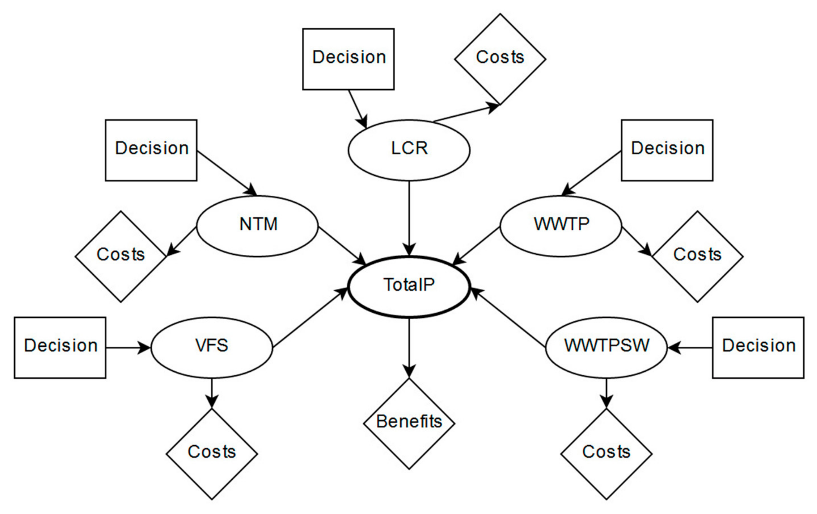
An influence diagram including the Bayesian network for the phosphorus abatement was designed based on dependencies among the variables. Figure 3 shows the final diagram structure. Ovals represent chance nodes, rectangles stand for decision nodes and rhombi for utility nodes. Arrows indicate causality between two variables. TotalP represents the variable of interest (probability of reducing the targeted amount of phosphorus).
3. Results
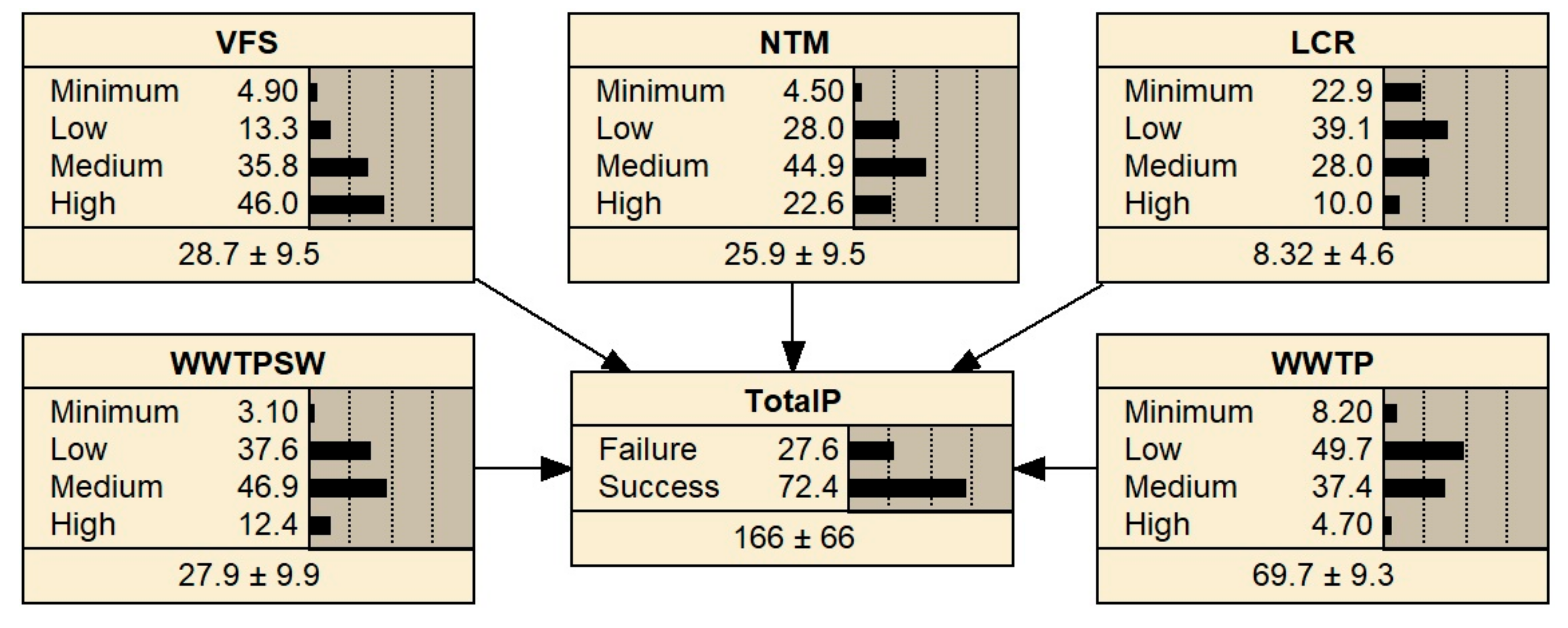
Probabilities obtained from the discretization were entered into the model. Simulation results are presented in Figure 4 with decision and utility nodes omitted for the sake of simplicity. Each interval has an assigned probability in percentage terms based on the modelling phase. The bottom line of each box shows the expected value of phosphorus reduced in kilograms and respective standard errors.
Unlike the groups of measures, TotalP was discretized into only two intervals based on the reduction target. Failure means that the required amount of phosphorus was not reduced, while Success indicates that more than the targeted amount of 148.82 kg was removed. Figure 4 shows that the “adjusted good status” will be achieved with a probability of 72.4%, which suggests that breaking the regulation is quite unlikely if the suggested measures are implemented. Some of the standard errors are quite high, but the analysis still provides more information than just one iteration in the deterministic analysis. Modifying the good status turned out to be a good option. Without BBT, CCR and cleaning of biological ponds, the remaining measures would reduce the original 200 kg target only in 2% of the cases.
It is also possible to see how effective the individual groups of measures are compared to how effective they were expected to be (see Table 1) or to find out what combination of groups of measures seems to be the most effective. To do so, one group of measures at a time is dropped and the kilograms of phosphorus which that group is expected to reduce are again subtracted from the “adjusted good status” (e.g., 26.45 is subtracted when VFS are dropped). If the resulting probability of success decreases, the combination of the remaining groups of measures is less effective than the group of measures which was removed, while the group of measures which was dropped overachieves. That seems to be the case of WWTP. When dropped, the probability of meeting the respective target falls to 65%. On the other hand, the probability of success for the remaining groups of measures rises to almost 76% when NTM are removed from the analysis, indicating that the variable has a lower potential than the other ones.
4. Discussion
In the context of the WFD, [25] argue that Bayesian networks are not suitable for environmental data, but they admit that the method corresponds with WFD logic as we are interested in whether the limits are satisfied, not by how much. On the other hand, Bayesian networks provide a robust way of determining whether the “good status” will be achieved in a specific water body. They also represent current knowledge of the system more realistically and can be updated without distorting the rest of the model thanks to conditional independencies [26]. There are both advantages and drawbacks to this approach (see [28] for a thorough discussion). First, one never gets a clear yes/no answer as the results are always probabilistic. The only way to be certain about the result is to aim for a 100% probability of success or zero. However, this is not desirable as that would mean the goal is achieved even when all the groups of measures are the least effective. The target would be met even if the effectiveness of all the groups of measures fell into the least effective section of the “minimum” interval, which is by itself very unlikely. If the target is met in such a situation, resources would be wasted in any other case. When the groups of measures are more effective, a smaller amount of the measures is required to achieve the “good status” at considerably lower costs. Therefore, careful consideration is needed when it comes to evaluating the results. Based on this, we see 72.4% of the 148.82 kg reduction as a reasonable number as the WFD requirements are broken in roughly a quarter of the cases and trying to achieve 100% is wasteful.
Computation of costs and benefits is quite unique in the case of achieving the “good status”. The costs are associated with implementation of the measures, meaning that the final number stays the same as in the case of deterministic analysis. However, information about the probability of achieving the “good status” is now available, which influences the calculation of benefits. It is very unlikely that the benefits grow linearly with a steady improvement in the water body status or in individual indicators that determine the status. It is more likely that some of the benefits are generated only when the “good status” is achieved. However, a significant amount of benefits is generated by visitors, and it is unlikely that a huge increase in benefits will occur once the water body already in a decent shape meets the last indicator and achieves the “good status”. Ideally, benefits associated with various levels of improvement should be estimated to make the comparison possible. This, however, is extremely difficult and time-consuming. It is not too problematic in the Stanovice case study. Macháč & Brabec [7] estimated that benefits of achieving the “good status” (EUR 289,136) are significantly larger than the costs of measure implementation (EUR 43,233). However, if the results of the CBA are closer, the benefits need to be revaluated. It should be noted that while complicated, this computation leads to more precise results. The deterministic CBA gives a clear answer but assumes that the implemented measures reduce exactly the targeted amount of phosphorus representing an unrealistic 100% probability of success. This is hardly true in reality and the Bayesian analysis presented in this paper confirms that. Therefore, benefits must be adjusted accordingly, but discussion of proper evaluation of benefits is not the subject of this paper.
The Bayesian approach is also more demanding on data availability. While the deterministic approach uses a fixed effectiveness for each measure within the same group (often based solely on expert judgement), the Bayesian method requires more empirical observations as a large sample is necessary for (ideally) representative discretization or at least probability distribution estimation. Allowing effectiveness within the group of measures to vary means that the analysis is closer to reality. It is confirmed by the collected data that similar measures do not always yield comparable results. First, not all the suggested measures in one group have the same parameters and are therefore likely to have different effectiveness. Moreover, local conditions also affect measure effectiveness and the fixed effectiveness cannot cover this variance. Expert judgement may also be used to substitute real data when the number of observations is unsatisfactory; see, e.g., [24]. This solution is not preferred but is possibly less distortive than using just a few observations as standard error is inversely related to sample size.
As indicated above, Bayesian networks may be used to test the “what if” type of questions [33]. In this case, the question is how much a particular group of measures contributes to achieving the target while maintaining the robustness. This could prove useful for measure selection. In the case study, the probability of meeting the respective target increases when NTM are dropped and their expected reduction is subtracted from the target. This indicates that NTM are less effective than other measures. Therefore, it may be efficient to go through the measure selection process again and handicap the ineffective measures. That means the expected effectiveness in Table 1 would be lowered for measures in the NTM group but increased for measures such as WWTP. This method is more time-consuming, just like the whole Bayesian approach, but may be economically desirable as fewer measures may be needed in the end. We recommend adjusting the selection process based on the results of the Bayesian analysis. Using the true effectiveness of measures may prevent wasting of resources on measures that might not be essential for achieving the target.
Bayesian networks are useful in assessing measure effectiveness, but they may be used to test uncertainty about costs and benefits as well. It might not make too much sense for costs of implementation as they are mostly dependent on market prices and the uncertainty is problematic mainly for large long-term investments (interest rate), but it can be useful for evaluation of benefits and for planning of measures in general. As Lansford & Jones [40] show, the largest part of benefits in water management (aesthetic, recreational, etc.) are not traded on markets and other techniques need to be used to estimate them correctly. Integrating the evaluation of benefits into the analysis should lead to accurate results, although they will again be probabilistic.
5. Conclusions
This paper applies the concept of Bayesian networks to decision making in water management. It helps to determine whether the “good status” required by the WFD can be achieved with a set of selected measures. Bayesian networks represent an effective way of assessing uncertainty of effectiveness of implemented measures, which can also be extended to costs and benefits and thus to proportionality analysis. The approach is presented on the case of the Stanovice water reservoir. Results of the case study show that the chosen measures eliminate the expected amount of phosphorus with a probability of 72.4%. Barton et al. [28] find that the phosphorus limits will be met with a probability of 56% in their case study on the Morsa catchment in Norway. That number is not dramatically different from the result presented here. However, they also find that agricultural measures dominate the model, which is contrary to our conclusions. On the other hand, most of the other authors predict that it will be hard to achieve the “good status” in the water bodies they studied, e.g., [29,33]. A straight comparison of the results is complicated, because each region and catchment area represents specific conditions. For example, the main source of phosphorus in the Morsa catchment is agriculture [28], which is contrary to the Stanovice case. Changes in the selection process might be desirable as some of the groups of measures exceed the original expectations about their effectiveness while other groups of measures fall short.
It is appropriate to incorporate the Bayesian approach into a proportionality analysis, which needs to be carried out if the water body applies for an exemption from achieving the “good status”. The approach should be used before conducting a CBA, because generated benefits heavily depend on achieving the “good status”. If the probability of breaking the regulation is high, more measures should be implemented and the whole process should be repeated until a higher probability is achieved. Thus, the economic assessment becomes more complex based on relevant biophysical aspects (effectiveness of measures) and the number of measures that lead to achieving the “good status”.
Bayesian networks are still used rather sparsely as they are demanding on data and not straightforward to interpret (especially in relation to the WFD). However, we believe this approach is informative and should be used more widely in water management. This paper offers an additional source of information for stakeholders who seek a more reliable way of assessing abatement measures in water management and planning and implementation of measures in catchments.
Supplementary Materials
The following are available online at https://www.mdpi.com/2073-4441/11/9/1791/s1, Table S1: Data used in the analysis.
Author Contributions
Conceptualization, J.J.; data curation, J.B. and J.M.; formal analysis, J.B. and J.M.; methodology, J.B. and J.M.; supervision, J.J.; writing—original draft, J.B.; writing—review & editing, J.M. and J.J.
Funding
This work was supported by the project Smart City—Smart Region—Smart Community (grant number: CZ.02.1.01/0.0/0.0/17_048/0007435, Operational Programme Research, Development and Education of the Czech Republic) and the project Specific Academic Research Projects 2019 of the Charles University, Faculty of Humanities, No. 260 471.
Acknowledgments
We would like to express our gratitude to the representatives of wastewater treatment plants that allowed us to use the anonymized data on plants’ effectiveness.
Conflicts of Interest
The authors declare no conflict of interest. The funding sponsors had no role in the design of the study; in the collection, analysis, or interpretation of data; in the writing of the manuscript, and in the decision to publish the results.
References
- Paerl, H.W.; Fulton, R.S., III; Moisander, P.H. Harmful Freshwater Algal Blooms, With an Emphasis on Cyanobacteria. Sci. World J. 2001, 1, 76–113. [Google Scholar] [CrossRef] [PubMed]
- Dumont, E.; Williams, R.; Keller, V.; Voß, A.; Tattari, S. Modelling indicators of water security, water pollution and aquatic biodiversity in Europe. Hydrolog. Sci. J. 2012, 57, 1378–1403. [Google Scholar] [CrossRef] [Green Version]
- Brack, W.; Dulio, V.; Ågerstrand, M.; Allan, I.; Altenburger, R.; Brinkmann, M.; Bunke, D.; Burgess, R.M.; Cousins, I.; Eschler, B.I.; et al. Towards the review of the European Union Water Framework management of chemical contamination in European surface water resources. Sci. Total Environ. 2017, 576, 720–737. [Google Scholar] [CrossRef] [PubMed]
- Directive 2000/60/EC of the European Parliament and of the Council Establishing a Framework for Community Action in the Field of Water Policy. Available online: https://eur-lex.europa.eu/legal-content/EN/TXT/?uri=celex:32000L0060 (accessed on 25 June 2019).
- European Environment Agency. European Waters Assessment of Status and Pressures 2018. Available online: https://www.eea.europa.eu/publications/state-of-water (accessed on 2 July 2019).
- Bateman, I.J.; Brower, R.; Davies, H.; Day, B.H.; Deflandre, A.; Di Falco, S.; Georgiou, S.; Hadley, D.; Hutchins, M.; Jones, A.P.; et al. Analysing the Agricultural Costs and Non-market Benefits of Implementing the Water Framework Directive. J. Agric. Econ. 2006, 57, 221–237. [Google Scholar] [CrossRef]
- Macháč, J.; Brabec, J. Assessment of Disproportionate Costs According to the WFD: Comparison of Applications of two Approaches in the Catchment of the Stanovice Reservoir (Czech Republic). Water Resour. Manag. 2018, 32, 1453–1466. [Google Scholar] [CrossRef]
- Courtecuisse, A. Water Prices and Households’ Available Income: Key Indicators for the Assessment of Potential Disproportionate Costs Illustration from the Artois Picardie Basin (France). In Proceedings of the International Work Session on Water Statistics, Vienna, Austria, 20–22 June 2005. [Google Scholar]
- Klauer, B.; Mewes, M.; Sigel, K.; Unnerstall, H.; Görlach, B.; Bräuer, I.; Pielen, B.; Hollaender, R. Verhältnismäßigkeit der Maßnahmenkosten im Sinne der EG-Wasserrahmenrichtlinie—Komplementäre Kriterien zur Kosten-Nutzen-Analyse; Helmholtz Zentrum für Umweltforschung: Leipzig, Germany, 2007. [Google Scholar]
- Vinten, A.J.A.; Ortega, J.M.; Glenk, K.; Booth, P.; Balana, B.B.; MacLeod, M.; Lago, M.; Moran, D.; Jones, M. Application of the WFD cost proportionality principle to diffuse pollution mitigation: A case study for Scottish Lochs. J. Environ. Manag. 2012, 97, 28–37. [Google Scholar] [CrossRef] [PubMed]
- Galioto, F.; Marconi, V.; Raggi, M.; Viaggi, D. An Assessment of Disproportionate Costs in WFD: The Experience of Emilia-Romagna. Water 2013, 5, 1967–1995. [Google Scholar] [CrossRef] [Green Version]
- Jensen, C.L.; Jacobsen, B.H.; Olsen, S.B.; Dubgaard, A.; Hasler, B. A practical CBA-based screening procedure for identification of river basins where the costs of fulfilling the WFD requirements may be disproportionate—applied to the case of Denmark. J. Environ. Econ. Policy 2013, 2, 164–200. [Google Scholar] [CrossRef]
- Klauer, B.; Sigel, K.; Schiller, J.; Hagemann, N.; Kern, K. Unverhältnismäßige Kosten Nach EG-Wasserrahmenrichtlinie—Ein Verfahren zur Begründung Weniger Strenger Umweltziele; Helmholtz-Zentrum für Umweltforschung—UFZ Department Ökonomie: Leipzig, Germany, 2015; ISSN 0948-9452. [Google Scholar]
- Slavíková, L.; Vojáček, O.; Macháč, J.; Hekrle, M.; Ansorge, L. Metodika k Aplikaci výjimek z důvodu nákladové nepřiměřenosti opatření k dosahování dobrého stavu vodních útvarů; (Methodology of Exemption Application in Case of Cost-disporoportionality of Achieving the “Good Status” on Water Bodies); Výzkumný ústav vodohospodářský T. G. Masaryka, v.v.i.: Praha, Czech Republic, 2015; ISBN 978-80-87402-41-2. [Google Scholar]
- Martin-Ortega, J.; Perni, A.; Jackson-Blake, L.; Balana, B.B.; Mckee, A.; Dunn, S.; Helliwell, R.; Psaltopoulos, D.; Skuras, D.; Cooksley, S.; et al. A transdisciplinary approach to the economic analysis of the European Water Framework Directive. Ecol. Econ. 2015, 116, 34–45. [Google Scholar] [CrossRef] [Green Version]
- Berbel, J.; Martin-Ortega, J.; Mesa, P. A Cost-Effectiveness Analysis of Water-Saving Measures for the Water Framework Directive: The Case of the Guadalquivir River Basin in Southern Spain. Water Resour. Manag. 2011, 25, 623–640. [Google Scholar] [CrossRef]
- Heckerman, D. A Tutorial on Learning with Bayesian Networks. In Innovations in Bayesian Networks; Holmes, D., Jain, L., Eds.; Springer: Berlin, Germany, 2008; Volume 156, pp. 33–82. [Google Scholar]
- Heckerman, D. Learning with Bayesian Networks. Lecture, 2016. Available online: https://slideplayer.com/slide/4998179/ (accessed on 27 June 2019).
- Briggs, A. A Bayesian approach to stochastic cost-effectiveness analysis. Health Econ. 1999, 8, 257–261. [Google Scholar] [CrossRef]
- Horvitz, E.; Breese, J.; Heckerman, D.; Hove, D.; Rommelse, D. The Lumiere Project: Bayesian User Modeling for Inferring the Goals and Needs of Software Users. In Proceedings of the Fourteenth Conference on Uncertainty in Artificial Intelligence, Madison, WI, USA, 24–26 July 1998; Morgan Kaufmann Publishers: Burlington, MA, USA, 1998. [Google Scholar]
- Heckerman, D.; Horvitz, E.; Nathwani, B. Toward Normative Expert Systems: Part I, The Pathfinder Project. Methods Inf. Med 1992, 31, 90–105. [Google Scholar] [CrossRef] [PubMed]
- Nadi, F.; Agogino, A.M.; Hodges, D.A. Use of Influence Diagrams and Neural Networks in Modeling Semiconductor Manufacturing Processes. IEEE Trans. Semicond. Manuf. 1991, 4, 52–58. [Google Scholar] [CrossRef]
- Hamilton, G.S.; Fielding, F.; Chiffings, A.W.; Hart, B.T.; Johnstone, R.W.; Mengersen, K. Investigating the Use of a Bayesian Network to Model the Risk of Lyngbya majuscula Bloom Initiation in Deception Bay, Queensland. Hum. Ecol. Risk Assess. 2007, 13, 1271–1287. [Google Scholar] [CrossRef]
- Ames, D.P.; Neilson, B.T.; Stevens, D.K.; Lall, U. Using Bayesian networks to model watershed management decisions: An East Canyon Creek case study. J. Hydroinform. 2005, 7, 267–282. [Google Scholar] [CrossRef]
- Fernandes, J.A.; Kauppila, P.; Uusitalo, L.; Fleming-Lehtinen, V.; Kuikka, S.; Pitkänen, H. Evaluation of Reaching the Targets of the Water Framework Directive in the Gulf of Finland. Environ. Sci. Technol. 2012, 46, 8220–8228. [Google Scholar] [CrossRef] [PubMed]
- Borsuk, M.E.; Stow, C.A.; Reckhow, K.H. A Bayesian network of eutrophication models for synthesis, prediction and uncertainty analysis. Ecol. Model. 2004, 173, 219–239. [Google Scholar] [CrossRef]
- Ticehurst, J.L.; Newham, L.T.H.; Rissik, D.; Letcher, R.A.; Jakeman, A.J. A Bayesian network approach for assessing the sustainability of coastal lakes in New South Wales, Australia. Environ. Model. Softw. 2007, 22, 1129–1139. [Google Scholar] [CrossRef]
- Barton, D.; Saloranta, T.; Moe, S.; Eggestad, H.; Kuikka, S. Bayesian belief networks as a meta-modelling tool in integrated river basin management—Pros and cons in evaluating nutrient abatement decisions under uncertainty in a Norwegian river basin. Ecol. Econ. 2008, 66, 91–104. [Google Scholar] [CrossRef]
- Moe, S.J.; Haande, S.; Couture, R.M. Climate change, cyanobacteria blooms and ecological status of lakes: A Bayesian network approach. Ecol. Model. 2016, 337, 330–347. [Google Scholar] [CrossRef] [Green Version]
- Maldonado, A.D.; Aguilera, P.A.; Salmerón, A. Continuous Bayesian networks for probabilistic environmental risk mapping. Stoch. Environ. Res. Risk Access. 2016, 30, 1441–1455. [Google Scholar] [CrossRef]
- Lindén, E.; Lehikoinen, A.; Kotta, J.; Aps, R.; Pitkänen, H.; Räike, A.; Korpinen, P.; Kuikka, S. EVAGULF—Protection of the aquatic communities in the Gulf of Finland: Risk-based policymaking. In Proceedings of the 2008 IEEE/OES US/EU-Baltic International Symposium, Tallinn, Estonia, 27–29 May 2008. [Google Scholar]
- Helle, I.; Vanhatalo, J.; Rahikainen, M.; Mäntyniemi, S.; Kuikka, S. Integrated Bayesian risk analysis of ecosystem management in the Gulf of Finland, the Baltic Sea—How to do it? Int. Counc. Explor. Sea CM 2012/I 2012, 4, 17–21. [Google Scholar]
- Lehikoinen, A.; Helle, I.; Klemola, E.; Mäntyniemi, S.; Kuikka, S.; Pitkänen, H. Evaluating the impact of nutrient abatement measures on the ecological status of coastal waters: A Bayesian network for decision analysis. Int. J. Multicriteria Decis. Mak. 2014, 4, 114–134. [Google Scholar] [CrossRef]
- Povodí Ohře. List Hodnocení Útvaru Povrchových Vod ID 113020300001 (Evaluation Sheet of Surface Water Body ID 113020300001) 2009. Available online: http://www.poh.cz/VHP/pop/C/5_LISTY_HODNOCENI/UTVARY_POVRCHOVYCH_VOD/113020300001.pdf (accessed on 12 January 2019).
- Dostál, T.; Krása, J. Opatření Pro Snížení Transportu Splavenin ze Zemědělské Půdy v Povodí Vodních Nádrží—Základní Charakteristika a Ekonomické Hodnocení Nákladů Spojených s Jejich Realizací (Measures for Reduction of Runoff from Farmland in Water Reservoir Catchment—Basic Characteristics and Economic Evaluation of Costs Associated with Implementation)—Output of Project TA02020808—Metody Optimalizace Návrhu Opatření v Povodí Vodních Nádrží Vedoucí k Účinnému Snížení Jejich Eutrofizace; ČVUT and IREAS: Prague, Czech Republic, 2014. [Google Scholar]
- Ansorge, L.; Drozd, P. Analýza Obcí v Povodí VN Stanovice (Analysis of Municipalities in Stanovice Water Reservoir Catchment); Internal document in the research project TA02020808; T. G. M. Water Research Institute: Prague, Czech Republic, 2014. [Google Scholar]
- Macháč, J.; Slavíková, L. Appropriateness of Cost-Effectiveness Analysis in Water Management: A Comparison of Cost Evaluations in Small and Large Catchment Areas. In Proceedings of the 20th International Conference Current Trends in Public Sector Research 2016, Šlapanice u Brana, Czech Republic, 21–22 January 2016; Špalková, D., Matějová, L., Eds.; Masaryk University: Brno, Czech Republic, 2016; pp. 302–309. [Google Scholar]
- Yu, J.; Smith, V.A.; Wang, P.P.; Hartemink, A.J.; Jarvis, E.D. Advances to Bayesian network inference for generating causal networks from observational biological data. Bioinformatics 2004, 20, 3594–3603. [Google Scholar] [CrossRef] [PubMed] [Green Version]
- Death, R.; Death, F.; Stubbington, R.; Joy, M.; van den Belt, M. How good are Bayesian belief networks for environmental management? A test with data from an agricultural river catchment. Freshw. Biol. 2015, 60, 2297–2309. [Google Scholar] [CrossRef] [Green Version]
- Lansford, N.H.; Jones, L.L. Recreational and Aesthetic Value of Water Using Hedonic Price Analysis. J. Agric. Resour. Econ. 1995, 20, 341–355. [Google Scholar]
Figure 1.
Location of Stanovice water reservoir.

Figure 2.
Essential methodology steps in Bayesian network application.

Figure 3.
Influence diagram of phosphorus abatement including the Bayesian network.

Figure 4.
Results of the Bayesian network showing probability of achieving the “good status”.


Table 1.
Measures entering the cost-effectiveness analysis and selected most efficient measures that theoretically reduce 200 kg/year of phosphorus inflows.
Table 1.
Measures entering the cost-effectiveness analysis and selected most efficient measures that theoretically reduce 200 kg/year of phosphorus inflows.
| Measure Type | Number of Identified Measures | Reduction from Identified Measures (kg/year) | Number of Selected Measures | Reduction from Selected Measures (kg/year) | Expected Effectiveness of Selected Measures |
|---|---|---|---|---|---|
| Broad-base terraces (BBT) | 27 | 21.06 | 4 | 6.03 | 70% |
| Vegetated filter strips (VFS) | 46 | 33.99 | 34 | 26.45 | 60–75% |
| Changes in crop rotation (CCR) | 48 | 26.15 | 16 | 11.79 | 50% |
| Leaving crop residue (LCR) | 48 | 15.69 | 13 | 5.67 | 30% |
| No-tillage methods (NTM) | 49 | 32.83 | 27 | 26.36 | 60% |
| Wastewater treatment plant (WWTP) construction/intensification (increasing of phosphorus reduction) | 5 1 | 93.91 1 | 3 | 64.44 | 100% |
| WWTP + sewerage system (SW) construction | 6 1 | 176.63 1 | 1 | 25.90 | 100% |
| Cleaning of biological ponds | 5 1 | 38.68 1 | 1 | 33.40 | 100% |
| Other measures on point sources (e.g., construction of sewage tanks) | 10 1 | 81.78 1 | 0 | 0 | 30–100% 2 |
| Total | 244 1 | 344.56 3 | 99 | 200.04 |
1 The measures on point sources consist of 4 different groups of measures. Implementation of these measures is often mutually exclusive: Implementation of a measure in one group prevents the implementation of a measure from another group. 2 Range of expected effectiveness for the whole group of measures. Measures in this category were not selected using the CEA based on the effect-cost ratio. 3 Due to the mutual exclusivity of some measures, the total amount of phosphorus that can be reduced by a combination of the listed measures does not correspond to the sum of total amounts of phosphorus that individual groups of measures can reduce by themselves.
Table 2.
Descriptive statistics of collected and simulated data for measures entering the analysis.
| Observation | VFS | NTM | LCR | WWTP | WWTP+SW |
| Mean (kg) | 28.60 | 26.16 | 8.27 | 69.97 | 27.88 |
| Median (kg) | 30.60 | 27.66 | 8.32 | 69.63 | 27.83 |
| Minimum (kg) | 6.03 | 2.63 | 1.13 | 51.18 | 8.72 |
| Maximum (kg) | 42.24 | 39.51 | 16.63 | 86.19 | 47.07 |
| Standard deviation (kg) | 9.06 | 8.84 | 4.55 | 8.09 | 8.39 |
| Observations | 68 | 19 | 23 | 65 | 77 |
| Distribution type | Johnson transformation | Normal | Normal | Normal | Normal |
| Simulation | VFS | NTM | LCR | WWTP | SEWERAGE |
| Mean (kg) | 28.71 | 26.07 | 8.20 | 69.59 | 27.81 |
| Median (kg) | 30.47 | 26.24 | 8.11 | 69.41 | 27.46 |
| Minimum (kg) | 0.00 | 0.00 | 0.00 | 43.30 | 0.93 |
| Maximum (kg) | 41.88 | 43.90 | 18.90 | 95.76 | 55.80 |
| Standard deviation (kg) | 8.92 | 8.9 | 4.44 | 8.24 | 8.33 |
| Observations | 1000 | 1000 | 1000 | 1000 | 1000 |
Table 3.
Effectiveness intervals for groups of measures entering the analysis and their probabilities.
Table 3.
Effectiveness intervals for groups of measures entering the analysis and their probabilities.
| Measure | Minimum | Low | Medium | High |
|---|---|---|---|---|
| VFS (kg) | [0, 10.5] | (10.5, 21] | (21, 31.5] | (30, 42] |
| Probability | 0.049 | 0.133 | 0.358 | 0.46 |
| NTM (kg) | [0, 11] | (11, 22] | (22, 33] | (33, 44] |
| Probability | 0.045 | 0.280 | 0.449 | 0.226 |
| LCR (kg) | [0, 4.75] | (4.75, 9.5] | (9.5, 14.25] | (14.25, 19] |
| Probability | 0.229 | 0.391 | 0.28 | 0.1 |
| WWTP (kg) | [46, 58.5] | (58.5, 71] | (71, 83.5] | (83.5, 96] |
| Probability | 0.082 | 0.497 | 0.374 | 0.047 |
| WWTP+SW (kg) | [0, 12.75] | (12.75, 25.5] | (25.5, 38.25] | (38.25, 51] |
| Probability | 0.031 | 0.376 | 0.469 | 0.124 |
© 2019 by the authors. Licensee MDPI, Basel, Switzerland. This article is an open access article distributed under the terms and conditions of the Creative Commons Attribution (CC BY) license (http://creativecommons.org/licenses/by/4.0/).
Share and Cite
MDPI and ACS Style
Brabec, J.; Macháč, J.; Jílková, J. Using Bayesian Networks to Assess Effectiveness of Phosphorus Abatement Measures under the Water Framework Directive. Water 2019, 11, 1791. https://doi.org/10.3390/w11091791
AMA Style
Brabec J, Macháč J, Jílková J. Using Bayesian Networks to Assess Effectiveness of Phosphorus Abatement Measures under the Water Framework Directive. Water. 2019; 11(9):1791. https://doi.org/10.3390/w11091791
Chicago/Turabian StyleBrabec, Jan, Jan Macháč, and Jiřina Jílková. 2019. "Using Bayesian Networks to Assess Effectiveness of Phosphorus Abatement Measures under the Water Framework Directive" Water 11, no. 9: 1791. https://doi.org/10.3390/w11091791
Note that from the first issue of 2016, this journal uses article numbers instead of page numbers. See further details here.