Article

Predicting Lake Quality for the Next Generation: Impacts of Catchment Management and Climatic Factors in a Probabilistic Model Framework

by
S. Jannicke Moe
1,*,
Raoul-Marie Couture
2,
Sigrid Haande
1,
Anne Lyche Solheim
1 and
Leah Jackson-Blake
1
1
Norwegian Institute for Water Research (NIVA), Gaustadalléen 21, 0349 Oslo, Norway
2
Department of Chemistry, Université Laval, 1045, av. de la Médecine, Québec City, QC G1V 0A6, Canada
*
Author to whom correspondence should be addressed.
Water 2019, 11(9), 1767; https://doi.org/10.3390/w11091767
Submission received: 30 June 2019 / Revised: 9 August 2019 / Accepted: 21 August 2019 / Published: 24 August 2019
(This article belongs to the Special Issue Water Quality and Ecosystems in Times of Climate Change)

Abstract

:
Lake ecosystems across the world are under combined pressures of eutrophication and climate change, which increase the risk of harmful cyanobacteria blooms, reduced ecological status, and degraded ecosystem services. In Europe, the third cycle of river basin management plans (2021–2027) according to the Water Framework Directive must take into account the potential impacts of climate change on water quality, including effects on relevant biological indicators. Here, we applied a Bayesian network as a meta-model for linking future climate and land-use scenarios for the time horizon 2050–2070, via process-based catchment and lake models, to cyanobacteria abundance and ecological status of a eutrophic lake. Building upon previous applications of the model, a new version was developed to include relevant climatic variables such as wind speed. Explorative scenarios showed that the combination of low wind and high temperature gave the most synergistic effects on cyanobacteria under high levels of eutrophication (Chl-a concentration). Considering the management target of good ecological status, however, the climate-related promotion of cyanobacteria blooms contributed most to degrading the ecological status at intermediate levels of eutrophication. Future developments of this model will aim to strengthen the link between climate variables and ecological responses, to make the model also useful for seasonal forecasting.

1. Introduction

Humans rely on freshwaters to provide a number of key services, such as water for drinking and agricultural irrigation, effluent dilution, hydropower generation, industrial cooling, fishing, and recreation. As a result of urbanization, population growth, and agricultural intensification, freshwaters have become the most threatened ecosystem type in large parts of the world, suffering historic and on-going widespread declines in the quantity and quality of habitats and the abundance of many species [1,2]. Harmful cyanobacterial blooms are becoming more common and widespread, and due to the toxins produced by many bloom-forming species, they are of particular concern for drinking water supplies, fisheries, and recreation [3,4].
Future generations can expect to experience more frequent harmful cyanobacterial blooms due to a warming climate and continued eutrophication [5]. Predictions of how the frequency and severity of cyanobacterial blooms are likely to change towards the middle of this century are of great interest, potentially allowing the development of site-specific catchment management plans to mitigate or adapt to predicted changes. However, to predict future conditions, we first need to understand the key factors controlling bloom occurrence, before we can then predict how these factors may change in the future as land use and climate change. In a recent review, Burford et al. [5] highlighted the need for observations and models which capture the role of both eutrophication and a changing climate.
The EU Water Framework Directive (WFD) [6] is the major policy driver for improving the condition of European freshwaters. The WFD requires that all waterbodies achieve at least “Good” ecological status by 2027, and requires River Basin Management Plans (RBMPs) to be developed to monitor and report current status and develop measures to achieve goals [7]. A key feature of the WFD is the use of the catchment-scale as the management unit, thereby allowing for the integrated effect of all pressures on water bodies to be considered. In contrast to traditional water regulations, the WFD requires that assessments of water quality are primarily based on biological indicators of ecosystem integrity [8]. Another novel feature is the requirement to consider future adaptation to climate change within RBMPs [9]. Modelling of future potential changes in water quality under future scenarios of change can therefore help support RBMP development and WFD implementation [10].
Process-based models are commonly used to predict future changes in freshwater pressures, such as nutrient loading and lake water temperature, under climate and land management change. For example, within the EU FP7 project MARS (Managing Aquatic ecosystems and water Resources under multiple Stress) [11], the status of physico-chemical elements (e.g., total phosphorus and nitrogen) were simulated in 16 European catchments up to the end of the 21st century [12]. Whilst many process-based models exist to predict physical and chemical variables, the factors governing changes in biological and ecological indicators, which in some areas are of most relevance to the WFD, are generally not understood well enough to be incorporated into process-based models. Instead, empirical or data-driven models are often used. In recent years, Bayesian network (BN) modelling has become a popular tool in environmental assessment and management [13,14,15], and provides a powerful means of linking abiotic process-based models to biological water quality indicators. A BN has the ability to link all the key components in a model chain into a single meta-model that can be run more easily and quickly than the process-based model chain. The graphical structure can be visualized, communicated, and discussed with stakeholders who are not familiar with mathematical modelling. The modelling framework can also be expanded to include expert knowledge. Within the MARS project, BNs were used to predict biological indicators in five of the 16 catchments (in Norway, Finland, Denmark, The Netherlands, and Portugal) [16].
For the Norwegian case study catchment, a BN was developed to predict cyanobacterial blooms and ecological status of Lake Vansjø in southeast Norway [17]. The BN modelled the combined effects and interactions of nutrients and temperature, and provides a useful starting point for future predictions. Factors other than nutrients and temperature play important roles in controlling the occurrence and severity of cyanobacterial blooms, such as the size, alkalinity, and humic content of lakes [18,19]. Modelling of cyanobacterial blooms should therefore be adapted to the lake type. Moreover, cyanobacterial blooms have been observed to be more likely during periods of low wind speed [20], when increased stratification can occur [21]. Under future climate change these periods of low wind may become more likely: atmospheric stilling (reduced surface wind speeds) is a phenomenon observed globally. So, in addition to recent increases in surface air temperature, reduced wind speed needs to be considered when evaluating the influence of climate change on lake ecosystems [22]. Current climate models have low skill at forecasting future changes in wind, but sensitivity (‘what if’) analyses can usefully be conducted within plausible ranges, to predict outcomes under e.g., worst- and best-case wind scenarios.
Within this paper, we describe a new updated BN to predict cyanobacteria in Lake Vansjø in Norway, incorporating additional important explanatory variables (Figure 1). Adding more predictor variables poses difficulties when it comes to training the model using only a limited dataset of observed data, and so the new updated BN was parameterized using an alternative statistical technique to that used previously. The BN is then applied to predict potential future cyanobacterial blooms using the MARS story lines, a common set of scenarios representing future land-use and climate, adapted to the local conditions of the case study in dialogue with stakeholders. Finally, we consider potential future uses for the model, for example to produce seasonal predictions of cyanobacterial bloom risk.

2. Materials and Methods
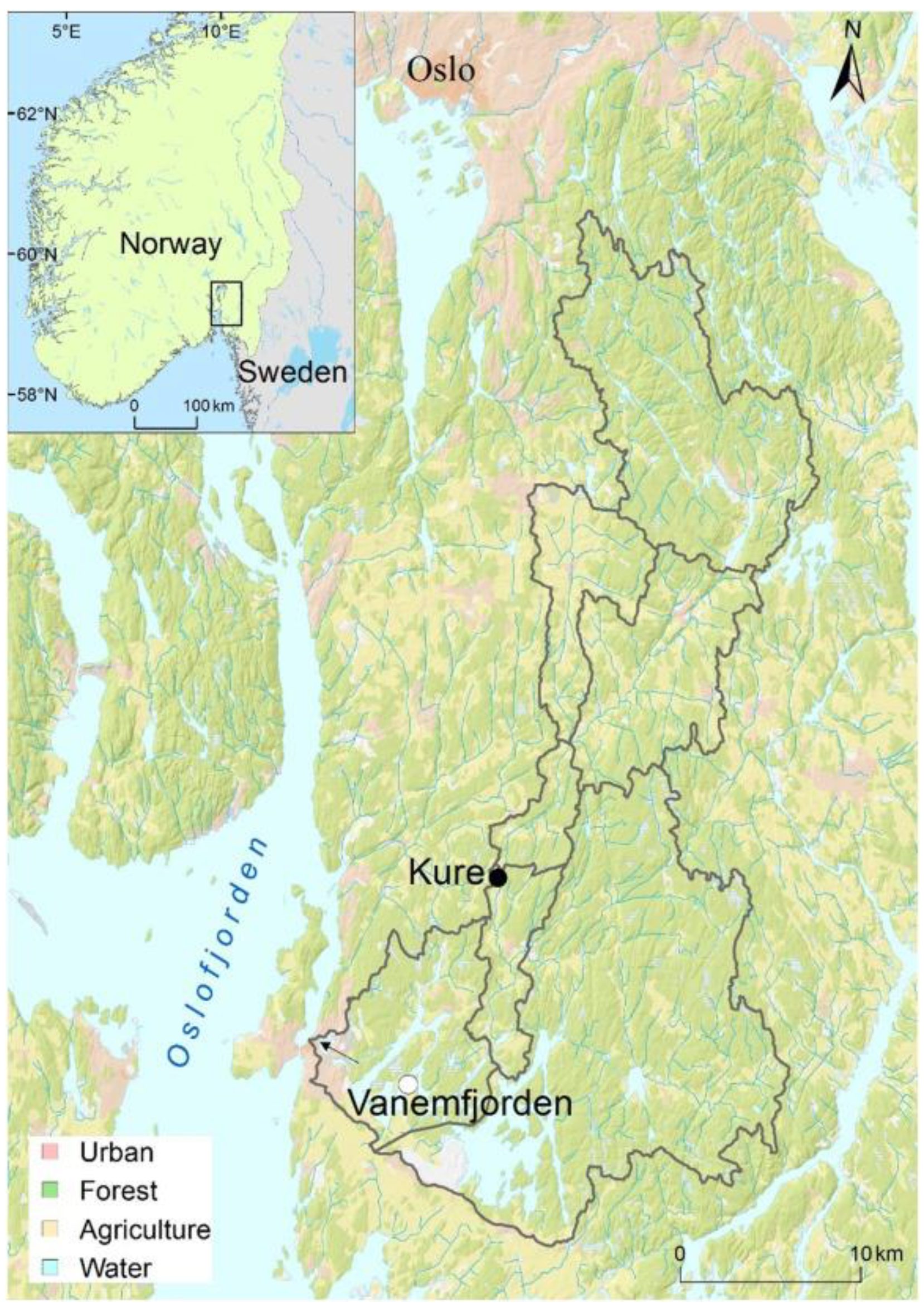
2.1. Case Study

Our case study is the Morsa catchment, consisting of the river Hobøl and lake Vansjø (Figure 2). The key pressures affecting water quality in this catchment are related to agriculture and climate change [23]. The catchment is one of the most agricultural in Norway, although land is still dominated by forestry (78%), with 15% agricultural land and 7% lakes. Agricultural land-use is mainly cereal production (89%), with small areas under grass (9.8%), vegetables (0.6%), and potatoes (<0.1%). Lake Vansjø is made up of two main sub-basins, Storefjorden in the east and Vanemfjorden in the west. Here, we focus on Vanemfjorden, which is shallower (max depth 19 m), has a much higher proportion of agriculture, especially vegetable crops, and is more susceptible to eutrophication and cyanobacterial blooms. All the following references to Lake Vansjø will refer to this basin. Agricultural activities contribute about 48% of the total phosphorus (P) input to the river basin, followed by natural runoff (39%), wastewater treatment plants (5%), and scattered dwellings (8%) [24]. The lake has a long history of eutrophication from at least the 1970s, when systematic monitoring of the lake began. Total P concentrations in Vanemfjorden lie between 20 and 40 μg/L P, above the threshold of 20 μg/L required for good ecological status according to the Water Framework Directive (Table 1) [25]. The lake, and in particular the basin Vanemfjorden, has suffered from toxin-producing cyanobacterial blooms, with bathing bans in place during much of the early 2000s, although these have been less frequent during the last decade [26].
A chain of process-based models has been set up and applied to simulate the key physical and chemical processes of the catchment (PERSiST and INCA-P) and lake (MyLake), all with daily temporal resolution. PERSiST [28] simulated the run-off in the river system, using inputs of catchment characteristics and time series of daily air temperature and precipitation. PERSiST was used to generate time series of soil moisture deficit and hydrologically effective rainfall (the rainfall contributing to runoff), which were then used to drive INCA-P. INCA-P [29] generated predictions of the river’s discharge and material transport, i.e., concentration of suspended solids, soluble reactive P, and total P. MyLake [30] used the predictions from INCA-P in combination with meteorological data to predict variables such as lake temperature, stratification, and concentrations of P fractions. The fraction of particulate organic P (POP) predicted by MyLake is used as a proxy for Chl-a, assuming that phytoplankton has a constant C:P ratio of 106:1 and a constant POP:Chl-a ratio of 1:1 [30]. Hence, this variable has a double role as an abiotic state (POP) predicted by MyLake and a biological indicator used in the lake classification system (Table 1).
This model chain was applied to simulate lake processes in Lake Vansjø for the future storylines defined in the MARS project [23]. The model chain can predict two important indicators of ecological status of lakes: Total P and Chl-a (Table 1). However, ecological status assessment of lakes in Northern Europe should also be based on the phytoplankton community composition, including the seasonal maximum cyanobacteria concentration [31]. Cyanobacteria abundance cannot yet be predicted by MyLake or other lake models that are suitable for Lake Vansjø, to our knowledge. Existing mechanistic lake models that predict cyanobacteria abundance, such as PROTECH [32], are not applicable because they cannot handle thermodynamics of Scandinavian lakes that freeze during winter. Therefore, we used a more empirical modelling approach, Bayesian networks [33,34,35], to link the abiotic model predictions to the most relevant biological indicators and onwards to the ecological status classes.

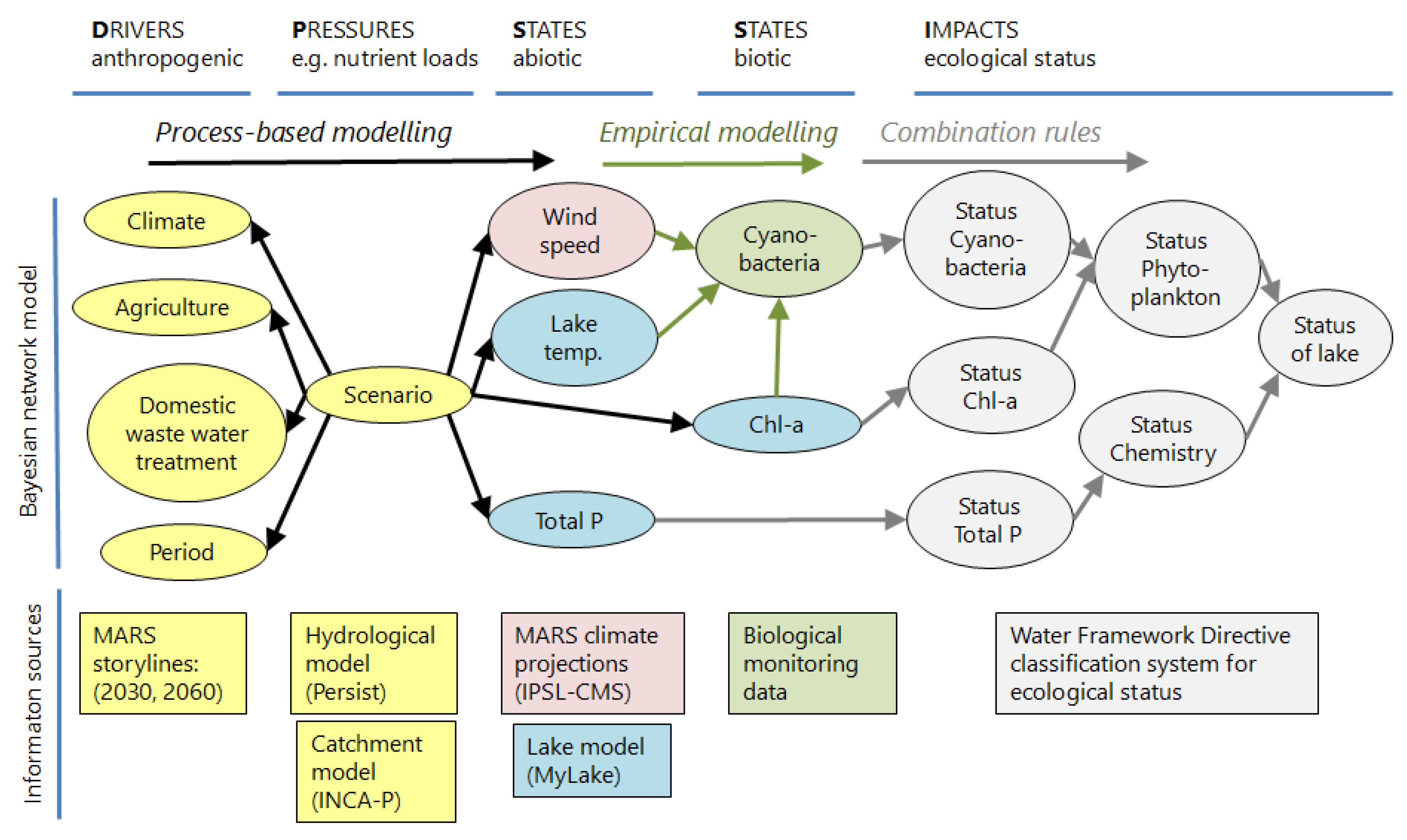
2.2. Bayesian Network as a Meta-Model for Future Storylines

In past EU projects REFRESH and MARS, we applied Bayesian network modelling as a meta-model for linking the outcome of process-based models (abiotic water quality) to biological indicators that are required for assessment of water quality according to the WFD [17,27]. The BN model was set up for Vanemfjorden in Lake Vansjø. (Previous BN models applied in this lake have focused on the less eutrophied Easter basin, Storefjorden) [37,38,39]. The conceptual meta-model for Lake Vansjø and its catchment has five modules (Figure 1):
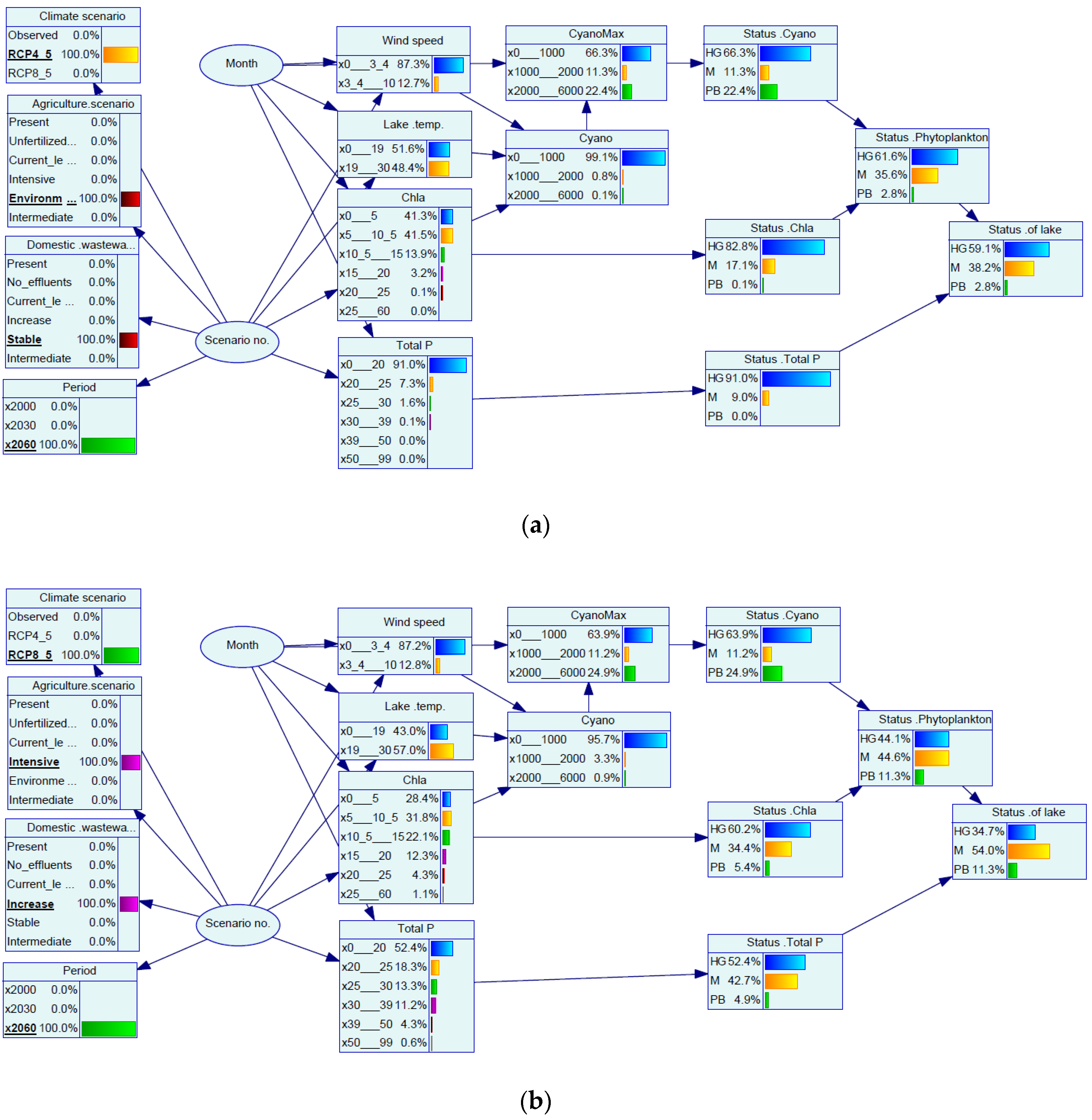
  • climate and management scenarios (yellow nodes),
  • output from the process-based lake model MyLake (blue nodes),
  • climatic data (red nodes),
  • monitoring data from Lake Vansjø (green nodes), and
  • the national classification system for ecological status of lakes (grey nodes).
In the current study, this approach was used to predict ecological status under the future storylines defined in the MARS project [11]. Within MARS, three storylines were constructed to project the impacts of multiple stressors on aquatic ecosystems under alternative plausible future conditions [40]: “Consensus World”, “Fragmented World”, and “Techno World” (Table 2). These storylines comprise multiple combinations of drivers and pressures for a given aquatic system for the current situation, and are shaped by future climatic scenarios (Representative Concentration Pathways-RCPs) and Shared Socioeconomic Pathways (SSPs).
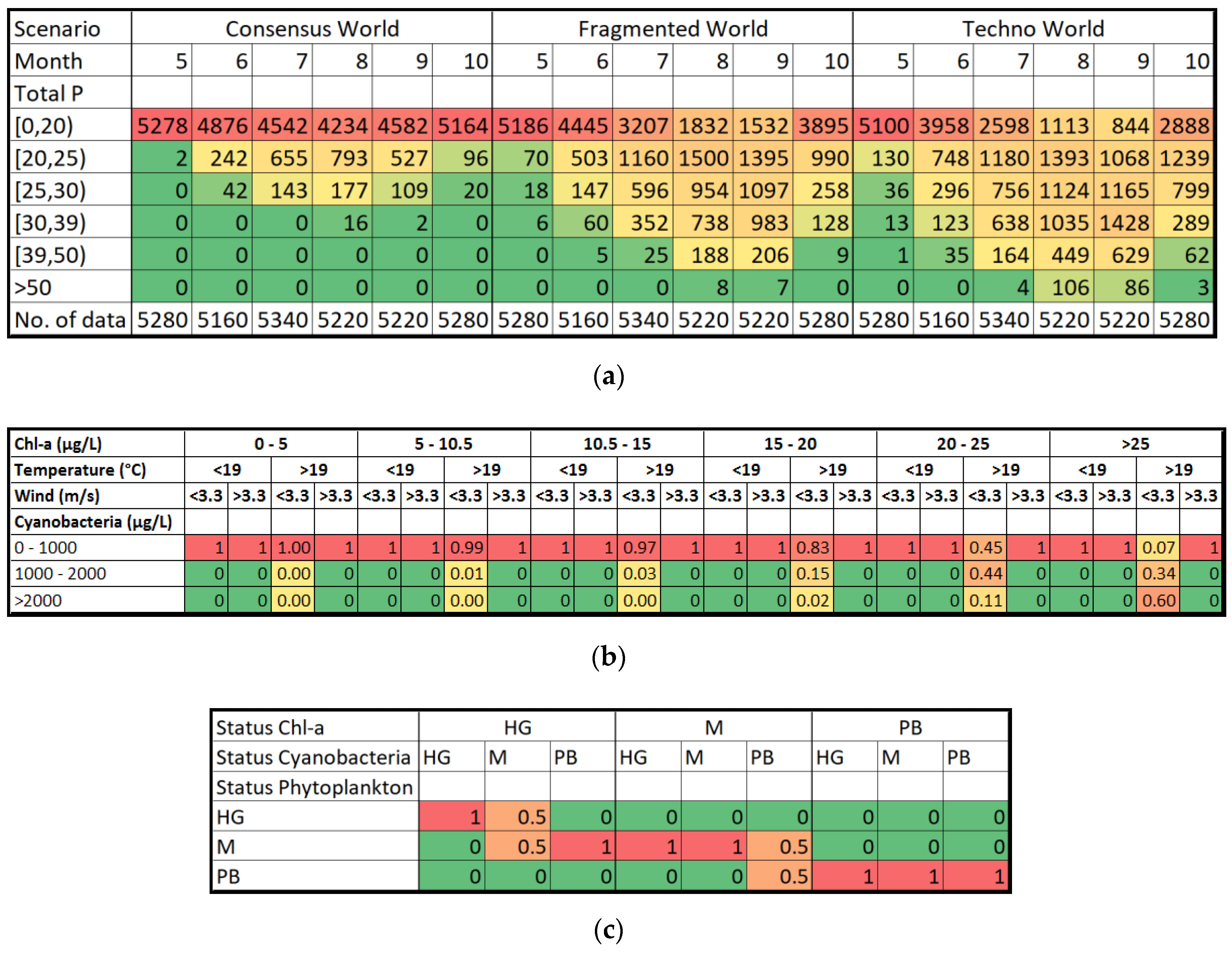
  • Consensus World (RCP4.5 and SSP2): the economy and population keep on growing, but environmental protection is prioritized. This is the best-case scenario for this case study.
  • Fragmented World (RCP8.5 and SSP3) is based upon inequality: each country needs to fight for its own survival and the environment is only protected locally by rich countries.
  • Techno World (RCP8.5 and SSP5) represents a future in which the world will be driven by economy. Policies are focused on enhancing trade and not on the environment. This is the worst-case scenario.
The specific implementation of each story line for the Vansjø catchment (Table 2) was evaluated in discussion with local stakeholders and water managers. This collaboration ensured that the implementation of the story lines would be based on expert knowledge including local pressures, climate impacts, and realistic mitigation measures. In this way, the storylines delivered a qualitative framework and, where possible, quantitative data for catchment and lake model simulations in seven European case study catchments [23].
Based on the downscaling of climate models and storylines to the Morsa catchment, future data were simulated by two climate models, IPSL (from Institut Pierre Simon Laplace) and GFDL (from Geophysical Fluid Dynamics Laboratory), and for the agricultural and water-related scenarios [27]. The future climate data contain daily values of air temperature, precipitation, wind, and other variables on a 0.5° × 0.5° grid, for the period 2006–2095. The process-based model chain provided predicted daily values for variable such as lake temperature, total P, and Chl-a for 25 scenarios in total (Table S16), representing different combinations of climate scenarios, climate models, management scenarios, and periods. For each scenario, MyLake generated 60 sets of simulated data, based on alternative parameter combinations.

2.3. Revised BN Model Structure

The development and application of the original BN model for Lake Vansjø (basin Vanemfjorden) under different scenarios are described by Moe et al. [17] and Couture et al. [27]. The latter version of the BN model took the MyLake outputs lake temperature, TP concentration, and Chl-a concentration as predictor variables.
In this study, the aim was to expand the BN model to more explicitly account for changes in key climatic variables. To achieve this, we explored the relationships between relevant lake monitoring data (lake temperature, Total P, Chl-a, cyanobacteria) and measured meteorological variables (air temperature, precipitation, and wind speed). Other potentially relevant stressor variables for the lake ecosystem, e.g., total nitrogen or water color (humic content), were not considered because these were not included in the process-based model MyLake. Therefore, it was not possible to predict these variables for the different scenarios with the process-based model chain. The process-based model MyLake was originally built for Lake Vansjø [30], assuming that it is a P-limited system, which is common for Northern European lakes. Another potentially relevant variable was Secchi depth, which could be estimated from the process-based lake model output. Secchi depth was nevertheless omitted from the BN model, because it is not used in the classification system for the given lake type (Table 1). The national classification guidance states that current class boundaries are not applicable for lakes with high turbidity, such as Lake Vansjø.
The monitoring data used for this analysis were downloaded from NIVA’s monitoring database through the user interface AquaMonitor (http://www.aquamonitor.no). The following data were included: water temperature (years 1993–1996, 2005–2013), Total P (1990–2013), Chl-a (1990–2013), and biomass of cyanobacteria (2004–2013). Integrated water samples from 0 to 4 m were collected for the chemical and biological analysis. The concentration of cyanobacteria were originally estimated as biovolume (mL/L). For each cyanobacteria species in a sample, the biovolume was estimated as the count of cells per unit water (cells/L) multiplied by the species-specific cell volume (mL/cell). By convention, concentration was reported as biomass (ug/L), assuming that the phytoplankton cells have the same density as water. From 2005 all variables were measured once per week, except for cyanobacteria, which were measured every two weeks. All monitoring data were aggregated to bi-weekly (14-days) average. Only data from the growing seasons months (May to October) were included in the model, in accordance with the national classification system.
Meteorological data were downloaded for the period 2007–2016 from the Norwegian Meteorological Institute (https://www.met.no/). The data included mean daily temperature, total precipitation, and wind speed measured at Rygge (meteorological station no. 17150). The meteorological data were aggregated to the same bi-weekly temporal scale as the monitoring data by average (temperature and wind speed) or by sum (precipitation).
The candidate explanatory variables for cyanobacteria were Chl-a and lake temperature (cf. [17]), as well as the new meteorological variables air temperature, wind speed, and precipitation. All statistical analyses were carried out in R, version 3.5.0 [41]. Relationships between meteorological data and lake monitoring data were explored by linear correlation, scatter plot smoothing, and regression trees. Linear correlation coefficients for all pairs of variables are displayed in the lower left panel of Figure 3, while the upper panel displays the data as scatter plots with smooth regression curves obtained by LOWESS (locally-weighted polynomial regression, [42]). The explanatory variables with highest linear correlation with cyanobacteria were Chl-a (r = 0.78) and lake temperature (r = 0.46). Air temperature had almost as high a correlation (r = 0.38), but also had a high correlation with water temperature (r = 0.89). Air temperature was therefore omitted from the BN model, since lake temperature was already a node in the BN model, and we assumed that lake temperature would have a more direct effect on the biology than air temperature. Although lake (and air) temperature showed smaller linear correlation with cyanobacteria than with Chl-a, the scatter plots indicated a stronger non-linear increase in cyanobacteria with high temperatures than for Chl-a. Conversely, for wind, the scatter plot displayed high cyanobacteria values only at low wind speeds. For precipitation, there was no strong linear correlation (all r < 0.22) or other systematic patterns (Figure 3). The revised candidate set of predictor variables for cyanobacteria were therefore Chl-a, lake temperature, and wind speed.
Discretization of continuous variables into intervals is a crucial step in the development of a traditional BN model with discrete nodes, since the method of discretization may strongly influence the model predictions [43]. Yet there is no consensus on how to select a method for discretization. We applied two main approaches to guide our decision on node intervals: (1) the class boundaries of the national classification system for ecological status of lakes [36] and (2) a statistical approach based on regression tree analysis. The class boundaries of Good/Moderate and Moderate/Poor status (Table 1) were used as intervals for the variables directly related to the quality elements used in the national classification system (Table 1): Total P, Chl-a, cyanobacteria, and CyanoMax. For Total P and Chl-a, a high number of values were simulated by the MyLake model, therefore the number of intervals could be doubled without compromising the parametrization of conditional probability tables (Section 2.4). The number of intervals was increased to six by splitting each of the three intervals at their midpoint.
For the remaining continuous variables (Lake temperature and Wind speed), regression tree analysis (R package Rpart) [44] was used to identify non-linearities and breakpoints in relationships between these variables and cyanobacteria (Figure 4). For lake temperature, the first significant split was at 18.98 °C (Figure 4a). This split gave a good balance of observations in the two branches (both n = 45), and the value 19 °C was chosen as the interval boundary. For wind speed (Figure 4b), the first significant split at 3.4 m/s resulted in one branch with 28 observations (higher wind speed) and one branch with 49 observations.
The selection of method for parametrization of conditional probability tables (CPT) is another critical step in the development of a BN model. In the original BN for Lake Vansjø [17], where the cyanobacteria node had two parent nodes (Chl-a and lake temperature), the CPT of this node was based on counts of observations. However, the addition of one more predictor variable (wind speed) would result in the doubling of the number of cells in the CPT from 18 to 36, and the number of observations (90) would not be sufficient for generating probability distributions merely based on counts. BN software offers other methods of quantifying CPTs based on sparse data, such as the expectation maximation algorithm [45]. Here, we used a statistical method: an ordinal regression method to estimate the probability of the three states of cyanobacteria status with the three parent nodes as predictor variables [46]. Ordinal regression is similar to logistic regression (where the response variable is 0/1), but allows for more than two ranked categories in the response variable (such as the ecological status classes High-Good, Moderate, and Poor-Bad), and estimates the cumulative probability of each state. We used the function “clm” (cumulative logit model) in the R package “ordinal” [47]. Lake temperature and wind were used as categorical predictor variables with two states (low/high) as specified above, while Chl-a was still used as a continuous predictor variable (it was not possible to have all three predictor variables as categorical) (Figure 5).
Comparison of nested ordinal regression models for the response variable cyanobacteria (Table 3) showed that wind speed alone was a better predictor than either Chl-a or lake temperature. The model with the lowest AIC value was no. 5, with Chl-a and wind speed as predictor variables. However, it was only marginally better (difference in AIC was less than 2) than model no. 6, which also contained lake temperature. We therefore chose to include all three variables as parent nodes for cyanobacteria in the revised BN model, to retain the ability for the model to explore effects of future increases in temperature.
The final BN model structure is shown conceptually in Figure 1 and described in Table 4. The Chl-a node is not linked directly to lake temperature and Total P in this model, although Chl-a abundance is commonly influenced by these variables in nature [48]. The reason is that the causal relationships between Total P and water temperature are modelled explicitly by the process-based MyLake model. These relationships are therefore represented implicitly by the arrows connecting the Scenarios and Chl-a nodes. The BN model was re-built in the software GeNIe version 2.2.2016.2 (https://www.bayesfusion.com/), the software chosen for collaborative BN modelling within the MARS project [16].

2.4. Parametrization of Conditional Probability Tables

The discrete probability distributions in the CPTs were obtained by different approaches in the different modules of the BN model (Figure 1) (see [17] for more details).
In Module 3 (climate), the conditional probability distribution of Wind speed (above or below 3.4 m/s) was calculated as the frequency distribution of these two states for each scenario and for each month of the year. In Module 2 (lake model output), likewise, the conditional probability distribution of each child node (Water temperature, Chl-a, and Total P) was calculated as the frequency distribution of this variable for each scenario and for each month. An example of a resulting CPT is shown in Figure 6a.
In Module 4 (biological monitoring data), we used the ordinal regression model for cyanobacteria (Section 2.3) to obtain the probability distribution for the different combinations of the parent nodes, using the predict function (predict.clm). To obtain a single input value for each interval of Chl-a (as required for the predict function), we used the median Chl-a concentration of each Chl-a interval (Figure 3). The resulting CPT for cyanobacteria is shown in Figure 6b. The CPT for CyanoMax (the maximum of cyanobacteria for each year; Table 1) was obtained by counting the number of observed cyanobacteria values in each concentration interval and each season, and calculating the frequency distribution across the corresponding CyanoMax intervals for all of these observations. For example, out of the 34 observations of cyanobacteria concentration below 1000 μg/L in the months May–June, 10 observations (29%) came from a year where the CyanoMax in the same year exceeded 2000 μg/L. Thus, even if the predicted cyanobacteria concentration for a single date in June is below 1000 μg/L, there is still a 29% probability that the CyanoMax value will be >2000 μg/L later that year.
In Module 5 (national classification system), the CPTs for ecological status are implementations of the rules defined by the national classification guidance (see [17]). An example is shown in Figure 6c. The BN assigns the probability of ecological status of the lake given estimates total P, Chl-a, and cyanobacteria abundance, according to the status class boundaries for each variable (Table 2). The ecological status is determined by two biological indicators (Chl-a and cyanobacteria) and one physico-chemical indicator (total P), using the following two combination rules: (1) if the cyanobacteria status is lower than Chl-a status, then the combined phytoplankton status is set to the average of the Chl-a and cyanobacteria. (If the cyanobacteria status is equal to or higher than the Chl-a status, then the cyanobacteria status is not included). (2) If the phytoplankton status is High or Good, and Total P status is lower than the phytoplankton status, then the combined lake status is reduced by one status class. (The status assessment of Chl-a and Total P based on individual months is not strictly correct, since the assessment should be based on the average of observations from the whole period May–October).
The CPTs of all nodes in the revised BN model are available in Supplementary Materials (Tables S1–S15).

2.5. Running the BN Model for Scenarios

The revised BN model was run for two types of scenarios: (1) explorative “what-if” scenarios based on weather conditions, and (2) future climate and management scenarios.

2.5.1. Explorative Scenarios

Four explorative what-if scenarios were defined by the different states of lake temperature (above/below 19 °C) and wind (above/below 3.4 m/s): Cold & Windy, Cold & Calm, Warm & Windy, and Warm & Calm (Table 5). A subset of the BN model (Modules 2–4) were run for these four scenarios in combination with six levels of eutrophication (Chl-a concentration). The purpose was to investigate the response of the cyanobacteria to these stressor combinations, and to identify stressor interactions.

2.5.2. Future Climate and Management Scenarios

In this study, we made use of the future climate and nutrient run-off data provided by the MARS scenarios to predict changes in ecological status under different scenarios for the time horizon 2060 (2050–2070). The BN model was run for the three MARS storylines (Consensus World, Fragmented World, and Techno World), as well as for scenarios with climate change only. Table 6 gives a summary of the output from the climate model and the process-based model chain [27], which served as input for the BN when run for these scenarios.

3. Results and Discussions

3.1. Effects of Explorative What-If Scenarios on Ecological Status

The combined effects of lake temperature, wind speed, and Chl-a concentration on cyanobacteria and phytoplankton status was explored for all possible combinations of the parent nodes, for the month of July. Two examples of combinations are shown in Figure 7: high (a) vs. low (b) wind speed in combination with high lake temperature and intermediate Chl-a concentrations. In all cases, the phytoplankton status was worse than the Chl-a status. This is due to the way phytoplankton status is determined by the Chl-a status in combination with the cyanobacteria status: the cyanobacteria status can contribute to reducing the phytoplankton status, but not improving it (cf. Figure 6c). In these examples, the probability of the seasonal maximum of cyanobacteria (CyanoMax) exceeding 1000 μg/L is always above zero, therefore the probability of high-good phytoplankton status will always be somewhat reduced by the probability of high cyanobacteria biomass.
The predicted probability distributions for cyanobacteria and phytoplankton status are summaries of a representative selection of the what-if scenarios in Figure 8. This figure illustrates that there was a strong interaction between the effects of the three stressors on the cyanobacteria status and the consequences for the total phytoplankton status. When the weather scenario was windy (Figure 8a), the probability of a cyanobacteria bloom is low (probability of Poor-Bad status is 14%). This result is not affected by the Chl-a concentration. The results shown in Figure 8a are also representative for the two scenarios Cold & Windy and Cold & Calm (not shown). In other words, increasing the level of eutrophication should not result in increased risk of cyanobacteria bloom as long as the weather conditions are unfavorable for cyanobacteria (cold and/or windy). For these scenarios, the total phytoplankton status (Figure 8b) mainly reflected the Chl-a concentration. When Chl-a was low (<10.5 µg/L), there was a 18% probability that high CyanoMax (>1000 µg/L) reduced the phytoplankton status from High-Good to Moderate. For intermediate Chl-a concentration (10.5–20 µg/L), there was 10% probability that even higher CyanoMax (>2000 µg/L) reduced the phytoplankton from Moderate to Poor-Bad. For the highest Chl-a concentration (>20 µg/L), the abundance of cyanobacteria could no longer contribute to reducing the combined phytoplankton status, which was already in the worst category (Poor-Bad).
When the weather scenario was Warm & Calm (Figure 8c), which is favorable for cyanobacteria, the probability of a cyanobacteria bloom increased abruptly with Chl-a concentration: the probability of CyanoMax exceeding 2000 µg/L increased from ca. 25% (lowest Chl-a concentration) to ca. 90% (highest Chl-a concentration). The consequences for the combined phytoplankton status (Figure 8d) was most pronounced for the intermediate Chl-a concentration (10.5–20 µg/L): the calm and warm weather conditions resulted in an increase in the probability of Poor-Bad status from ca. 10% to 20%. The lower Chl-a interval represented conditions where cyanobacteria blooms were not likely, while the higher Chl-a interval represented a situation where cyanobacteria blooms were likely but would not affect the already Poor-Bad ecological status.
Many studies of environmental factors promoting cyanobacteria have focused on the effects of nutrients in combination with high temperature [21,49]. The importance of stable water conditions and stratification (stability of the water column) is also well documented (e.g., [50]). A model of cyanobacteria blooms in New South Wales (Australia) suggested that increased stratification is more important than nutrients for cyanobacteria bloom formation [45]. However, predictive models for cyanobacteria have only recently taken into account the role of wind [3]. For example, a predictive model based on high-frequency lake monitoring data of water temperature, light, wind speed, and cyanobacterial fluorescence (a proxy for biomass) was able to successfully predict cyanobacterial fluorescence over the coming days and weeks [51].
In summary, the exploration of weather scenarios show that (1) the combination of high temperature and calm wind will promote high concentrations of cyanobacteria, (2) this stressor interaction has the strongest effect on cyanobacteria when Chl-a concentration is high, (3) but the effect of this stressor combination on the phytoplankton status is highest when Chl-a concentration is intermediate. Note that this assessment only considers the impacts of cyanobacteria in terms of the ecological status, as defined by the Water Framework directive. At higher levels of eutrophication (Chl-a concentrations), there is a higher risk of cyanobacterial blooms affecting ecosystem services such as drinking and bathing water quality [39,52], even if this is not manifested as a further reduction of ecological status.

3.2. Predicted Lake Quality under Future Story Lines

The full BN model was run for the three MARS storylines, as well as for climate and management scenarios separately, for the two time horizons 2030 (2020–2040) and 2060 (2050–2070). Here we present results from the BN model based on the climate model IPSL for the years 2050–2070. The updated probability distributions of all nodes are displayed for examples of the best-case and worst-case storylines: Consensus World (Figure 9a) and Techno World (Figure 9b), run for the month July. A summary of the BN model predictions for selected nodes are shown for a larger number of scenarios in Figure 10: the baseline scenario (i.e., current management practice extended to time horizon 2060), the two climate scenarios and the three storylines.
In the Techno World scenario (Figure 9a), more intensive agriculture and increased wastewater effluents in combination with higher climate gas emissions resulted in higher levels of eutrophication. Compared with the Consensus World scenario, the probability of meeting the management target (High-Good status) for Chl-a was reduced from 84% to 63%, while the corresponding probability for Total P was reduced from 93% to 58%. The climatic variables showed only a weak (and probably insignificant) change between the two storylines: the probability of warm days (lake temperature >19 °C) increased from 41.8% to 43.4%, while the probability of calm days (wind speed <3.4 m/s) was reduced from 86.7% to 81.9%. (The mean wind speed for the whole season, however, showed a slight increase; Table 2).
In contrast, the difference in cyanobacteria status between these storylines only weakly reflected the increase in Chl-a concentration. The BN results indicate that cyanobacteria concentrations show little response to changes in scenarios and storylines. One reason for this apparent lack of response by cyanobacteria is the discretization of the concentration gradient based on the status class boundaries (1000 and 2000 µg/L). The frequency of observed cyanobacteria concentrations >1000 μg/L in the monitoring data is quite low, even for the most favorable environmental conditions. The ordinal regression model is based on relatively few observations (103 samples), of which only 13 samples have cyanobacteria concentration exceeding 1000 µg/L. This implies that the CPT for cyanobacteria is associated with high uncertainty. As a result, the probabilities of different cyanobacteria states do not vary much between different scenarios. A cyanobacteria node with a finer discretization of the interval below 1000 µg/L would likely have displayed a stronger response within this range to increased Chl-a concentrations, even if the probability of blooms would not be affected. In future versions of the model, more sophisticated methods for parametrizing CPTs based on few data [14] could allow for a cyanobacteria node with higher resolution and possibly higher sensitivity to environmental change.
Moreover, the two climate scenarios had little difference in wind speed (Table 2, Figure 10a), therefore the probability distribution of the Wind speed node remained almost unaltered (Figure 9). The wind speeds predicted by the climate model were usually calm (ca. 90% of predicted values <3.4 m/s), while the observed meteorological data for Lake Vansjø had only 56% calm days. This mismatch was probably due to inadequacies in the downscaling of the climate model predictions to the local conditions of Lake Vansjø. Therefore, the stressor interaction between wind and lake temperature seen in exploratory scenarios (Figure 8) did not emerge in full BN runs for different future scenarios (Figure 10). The predicted status class distributions of this model are therefore consistent with the previous model version without wind speed [27]. However, it is still possible to explore alternative metrics of stability based on these meteorological data, such the number of consecutive calm days, which might reveal a stronger response of cyanobacteria to the future wind conditions.
Although cyanobacteria did not show a clear response to the scenarios in the study, this variable still has an important role in the overall status classification of the lake. Across all scenarios, cyanobacteria (Figure 10b) contributed to worsening the status assessed by phytoplankton (Figure 10e), compared to an assessment by Chl-a alone (Figure 10d); the latter assessment is typically the outcome of process-based models [23]. In this BN approach, the cyanobacteria status contributes to a more correct and more protective assessment of the overall response of phytoplankton status, and thereby of total lake status, to the scenarios.
Our model has assumed that the conditional probabilistic relationships among nodes stay the same under future scenarios, which may be violated e.g., when the underlying relationships are non-linear or influenced by other variables. For example, we assumed that the amount of cyanobacteria under future scenarios can be predicted by the increase in Chl-a, temperature, and wind. Interactions between environmental stressors are common in freshwater ecosystems [53], and synergistic interactions between warming and nutrient enrichment have been documented for cyanobacteria in lakes worldwide [54]. In the future, Lake Vansjø might experience longer periods of high temperature and calm weather than those recorded so far, which may potentially have a stronger synergistic effect on the cyanobacteria abundance than is captured in the current CPTs. Moreover, we have not accounted for other environmental conditions that can change with future climate and land use, such as changes in discharge, nitrogen and phosphorus run-off, and humic content. In this respect, the current BN can be considered a conservative model, which is more likely to underestimate than to overestimate changes in lake status under the future scenarios.

3.3. Assessment of the Bayesian Network Modelling Approach

During recent decades, Bayesian network models have been applied to analyze and predict the occurrence of potentially harmful cyanobacteria in lakes and coastal waters in many parts of the world. The examples show a great range of spatial scales, ranging from single case studies of individual lakes (e.g., [38]) to larger sets of lakes [55] and large coastal areas (e.g., [56]). Likewise, the temporal resolution of BN models for cyanobacteria span high-frequency models with real-time data [57] to seasonal forecast [58] and assessment for future decades (this study). This diversity of models suggests that the BN approach is useful for predicting the occurrence and abundance of cyanobacteria, across different scales and systems.
Nevertheless, the application of the BN methodology in the context of environmental management poses many challenges. The traditional non-dynamic networks cannot contain loops, which puts constraints on the ecological processes that can be modelled. Phosphorus and phytoplankton dynamics in lakes are typically dominated by feedback processes [30]. For example, high phytoplankton biomass can reduce the Secchi depth, which can in turn limit further phytoplankton growth due to light limitation. In our study, such feedback loops were handled by dynamic models (INCA-P and MyLake), while the BN summarized the outcome of the catchment and lake processes. Another challenge is the propagation of uncertainty. Although the explicit modelling of uncertainty or variability is a desirable property of BNs, the accumulation of uncertainty along the network means that the final output nodes of interest may show low sensitivity to changes in environmental conditions [46]. While a BN model can incorporate uncertainty for all variables, the predicted probability of a given state of a variable is still typically expressed as a single value, without a distribution or confidence interval. Therefore, it is not straightforward to evaluate the solidity of the calculated probabilities and to decide what should be considered a significant change in probability. Other limitations associated with the use of BNs in environmental science have been discussed elsewhere, e.g., [52,59].
For assessment of the ecological status of surface waters according to the WFD, the BN approach is an important supplement to the existing process-based models, providing an opportunity to include biological elements, as demonstrated in this study. Biological monitoring data are often sparse and costly compared to physico-chemical monitoring data, but theory or expert knowledge of selected biological indicators can be used as a first step to construct causal links (CPTs) between abiotic and biotic responses. This is clearly an added value for use of models in water management, at least in Europe where the WFD requires that assessments are based primarily on biology [8]. Moreover, the WFD requires that potential impacts of climate change are considered in the next cycle (2021–2026) of river basin management plans [9]. Much information can be found on the likely effects of climate change on specific taxonomic groups or environmental processes, but incorporating such information into predictive models remains a challenge. The BN methodology can facilitate the use of such knowledge, manifested as expert judgement of probabilities under given climatic scenarios.
A Bayesian network developed for integrating coastal eutrophication models [46] was able to accommodate a diversity of methods, and allowed for the prediction of more policy-relevant ecosystem attributes. Compared to process-based models, a BN model may be relatively easy to interpret for end users without training in modelling [60]. Therefore, BNs are promising tools for supporting informed decision making and thus the work of water managers [56].
Bayesian models more generally can have many of the benefits of BNs without the loss of information due to the discretization of nodes. For example, a Bayesian seasonal bloom forecast model for the Western Lake Erie Basin was extended to provide new regional predictions to reflect nearshore conditions or regional variations, which are important for local stakeholders [58]. By linking predictive basin-wide models to regional regression estimates the authors were able to better predict potential bloom impacts at scales and in specific areas that allow for better management responses. There is also rapid development within the field of BN modelling, and the more advanced versions such as hybrid BNs (containing continuous and discrete nodes), dynamic BNs, and integrated BNs [14] may overcome some of the shortcomings of traditional BNs. Nevertheless, their strengths will remain in exploration of “what-if” scenarios, and in being able to incorporate both expert knowledge and empirical data [14].

3.4. Conclusions and Outlook

In this paper, we have demonstrated the importance of climatic variables, in particular wind speed, for driving the probability of cyanobacterial blooms. Our explorative scenarios suggest that low wind speed in combination with high temperature reduce the probability of achieving the WFD-defined water management goals of Good ecological status, and to cause further degradation of lakes that have Moderate or worse status. The Bayesian network approach enabled linking of this biological indicator to future climate and management scenarios, for predicting ecological status of our case study lake for the time horizon 2050–2070. Although the class boundaries used for ecological status classification of lake Vansjø are specific for this lake type, the classification system is compliant with the WFD and the class boundaries are intercalibrated with other European lake classification systems [61]. Therefore, this modelling approach can easily be adapted to other lakes for which the same type of information is available.
The link between future climate scenarios and ecological responses in our study was weakened by the mismatch between modelled and observed data on wind speed. This link might be improved by a better downscaling and adjustment of the projected climate data to the catchment region in question, and by using climatic metrics with higher ecological relevance (e.g., the number of consecutive calm days). For further development of the BN model, we will continue to investigate options for parametrizing and updating the conditional probability table for cyanobacteria. For example, hierarchical Bayesian modelling of monitoring and meteorological data from other relevant lakes may provide a more representative CPT.
The discretization of continuous variables for discrete BN models typically lead to loss of precision and should ideally be avoided [43]. A longer-term goal is therefore to transform the model into a continuous-variable BN [62], to make more efficient use of the available information. In the current study, we have taken a first step in this direction, by letting the link from abiotic to biotic variables (cyanobacteria) be based on a statistical model instead of the counts of observations.
This BN model can also be adapted to predict the ecological status and the risk of not achieving management targets for short-term scenarios, such as within the next season. This is the aim of the on-going EU-funded project WATExR (https://watexr.eu/), which focuses on integration of climate seasonal prediction and ecosystem impact modelling for an efficient adaptation of water resources management to increasing climate extreme events. In practice, any forecasting of climatic variables such as wind and temperature for the coming season will have high uncertainty. Nevertheless, we can use for example the best- and worst-case weather projections (temperature and wind) in combination with the most recent monitoring and climate data available (e.g., Chl-a, Total P, precipitation and temperature) to predict a plausible range of outcomes (abundance of cyanobacteria and ecological status). In this way, an adapted version of our model has the potential to support river basin managers in making risk assessments and decisions that account for extreme climatic events.

Supplementary Materials

The following are available online at https://www.mdpi.com/2073-4441/11/9/1767/s1: A file named Tables_BN_Vansjo_2019-08-07.xlsx containing the conditional probability tables of all 15 child nodes in Table 1 as separate sheets. Table S1: Climate scenario, Table S2: Agricultural scenario, Table S3: Domestic wastewater scenario, Table S4: Period, Table S5: Wind speed, Table S6: Lake temperature, Table S7: Chl-a, Table S8: Total P, Table S9: Cyanobacteria, Table S10: CyanoMax, Table S11: Status Cyanobacteria, Table S12: Status Chl-a, Table S13: Status Phytoplankton, Table S14: Status Total P, Table S15: Status of lake. In addition, the file contains a description of the two root notes: Table S16: Scenario no., Table S17: Month.

Author Contributions

Conceptualization, S.J.M. and A.L.S.; Data curation, S.J.M. and S.H.; Formal analysis, S.J.M.; Funding acquisition, R.-M.C. and A.L.S.; Investigation, S.J.M., R.-M.C. and S.H.; Methodology, S.J.M., R.-M.C. and L.J.-B.; Project administration, L.J.-B. and A.L.S.; Software, S.J.M.; Visualization, S.J.M. and R.-M.C.; Writing—original draft, S.J.M. and L.J.-B.; Writing—review and editing, S.J.M., R.-M.C., S.H., L.J.-B. and A.L.S.

Funding

This research was funded by the projects MARS (EU FP7, Theme 6, contract no. 603378) and WATExR (part of ERA4CS, an ERA-NET initiated by JPI Climate, and funded by MINECO (ES), FORMAS (SE), BMBF (DE), EPA (IE), RCN (NO), and IFD (DK), with co-funding by the EU (contract no. 690462)).

Acknowledgments

We thank the participants of the MARS workshop on Bayesian network modelling of catchment case studies for useful discussions, especially Samu Mäntyniemi and David N. Barton.

Conflicts of Interest

The authors declare no conflict of interest. The funders had no role in the design of the study; in the collection, analyses, or interpretation of data; in the writing of the manuscript, or in the decision to publish the results.

References

  1. Gozlan, R.E.; Karimov, B.K.; Zadereev, E.; Kuznetsova, D.; Brucet, S. Status, trends, and future dynamics of freshwater ecosystems in Europe and central Asia. Inland Waters 2019, 9, 78–94. [Google Scholar] [CrossRef]
  2. Jeppesen, E.; Kronvang, B.; Meerhoff, M.; Søndergaard, M.; Hansen, K.M.; Andersen, H.E.; Lauridsen, T.L.; Liboriussen, L.; Beklioglu, M.; Özen, A.; et al. Climate change effects on runoff, catchment phosphorus loading and lake ecological state, and potential adaptations. J. Environ. Qual. 2009, 38, 1930–1941. [Google Scholar] [CrossRef] [PubMed]
  3. Ibelings, B.W.; Fastner, J.; Bormans, M.; Visser, P.M. Cyanobacterial blooms. Ecology, prevention, mitigation and control: Editorial to a CYANOCOST special issue. Aquat. Ecol. 2016, 50, 327–331. [Google Scholar] [CrossRef]
  4. Huisman, J.; Codd, G.A.; Paerl, H.W.; Ibelings, B.W.; Verspagen, J.M.H.; Visser, P.M. Cyanobacterial blooms. Nat. Rev. Microbiol. 2018, 16, 471–483. [Google Scholar] [CrossRef] [PubMed]
  5. Burford, M.A.; Carey, C.C.; Hamilton, D.P.; Huisman, J.; Paerl, H.W.; Wood, S.A.; Wulff, A. Perspective: Advancing the research agenda for improving understanding of cyanobacteria in a future of global change. Harmful Algae 2019. [Google Scholar] [CrossRef]
  6. EC (European Commission). Directive 2000/60/EC of the European Parliament and of the Council of 23 October 2000 Establishing a Framework for Community Action in the Field of Water Policy; Office for Official Publications of the European Communities: Luxembourg, 2000. [Google Scholar]
  7. EEA (European Environment Agency). European Waters. Assessment of Status and Pressures 2018; EEA Report No. 7/2018; Copenhagen, Denmark, 2018. [Google Scholar]
  8. EC (European Commission). Overall Approach to the Classification of Ecological Status and Ecological Potential;Common Implementation Strategy for the Water Framework Directive Guidance Document Number 13; Office for Official Publications of the European Communities: Luxembourg, 2005. [Google Scholar]
  9. EC (European Commission). River Basin Management in a Changing Climate. Common Implementation Strategy for the Water Framework Directive Guidance Document Number 24; Office for Official Publications of the European Communities: Luxembourg, 2009. [Google Scholar]
  10. Carvalho, L.; Mackay, E.B.; Cardoso, A.C.; Baattrup-Pedersen, A.; Birk, S.; Blackstock, K.L.; Borics, G.; Borja, A.; Feld, C.K.; Ferreira, M.T.; et al. Protecting and restoring Europe’s waters: An analysis of the future development needs of the water framework directive. Sci. Total Environ. 2019, 658, 1228–1238. [Google Scholar] [CrossRef]
  11. Hering, D.; Carvalho, L.; Argillier, C.; Beklioglu, M.; Borja, A.; Cardoso, A.C.; Duel, H.; Ferreira, T.; Globevnik, L.; Hanganu, J.; et al. Managing aquatic ecosystems and water resources under multiple stress—An introduction to the MARS project. Sci. Total Environ. 2015, 503, 10–21. [Google Scholar] [CrossRef]
  12. Ferreira, T.; Panagopoulos, Y.; Bloomfield, J.; Couture, R.-M.; Omerod, S.; Stefanidis, K.; Mimikou, M.; Hanganu, J.; Constantinescu, A.; Beklioğlu, M.; et al. Deliverable 4.1: Case Study Synthesis. 2016. Available online: http://www.mars-project.eu/files/download/deliverables/MARS_D4.1_case_study_synthesis.pdf. (accessed on 30 June 2019).
  13. Barton, D.N.; Kuikka, S.; Varis, O.; Uusitalo, L.; Henriksen, H.J.; Borsuk, M.; de la Hera, A.; Farmani, R.; Johnson, S.; Linnell, J.D.C. Bayesian networks in environmental and resource management. Integr. Environ. Assess. Manag. 2012, 8, 418–429. [Google Scholar] [CrossRef]
  14. Marcot, B.G.; Penman, T.D. Advances in bayesian network modelling: Integration of modelling technologies. Environ. Model. Softw. 2019, 111, 386–393. [Google Scholar] [CrossRef]
  15. Moe, S.J. Bayesian models in assessment and management. In Environmental Risk Assessment and Management from a Landscape Perspective; Kapustka, L., Landis, W.G., Johnson, A., Eds.; Wiley’s: Chicago, IL, USA, 2010. [Google Scholar]
  16. Van Geest, G.; Kramer, L.; Buijse, T.; Moe, J.; Couture, R.-M.; Lyche Solheim, A.; Molina-Navarro, E.; Andersen, H.E.; Trolle, D.; Rankinen, K.; et al. D7.2-2: Bayesian Belief Networks: Linking Abiotic and Biotic Data. 2017. Available online: http://www.mars-project.eu/files/download/deliverables/MARS_D7.2_MARS_suite_of_tools_2.pdf (accessed on 30 June 2019).
  17. Moe, S.J.; Haande, S.; Couture, R.-M. Climate change, cyanobacteria blooms and ecological status of lakes: A Bayesian network approach. Ecol. Model. 2016, 337, 330–347. [Google Scholar] [CrossRef] [Green Version]
  18. Carvalho, L.; McDonald, C.; de Hoyos, C.; Mischke, U.; Phillips, G.; Borics, G.; Poikane, S.; Skjelbred, B.; Lyche Solheim, A.; Van Wichelen, J.; et al. Sustaining recreational quality of European lakes: Minimizing the health risks from algal blooms through phosphorus control. J. Appl. Ecol. 2013, 50, 315–323. [Google Scholar] [CrossRef]
  19. Richardson, J.; Miller, C.; Maberly, S.C.; Taylor, P.; Globevnik, L.; Hunter, P.; Jeppesen, E.; Mischke, U.; Moe, S.J.; Pasztaleniec, A.; et al. Effects of multiple stressors on cyanobacteria abundance vary with lake type. Glob. Chang. Biol. 2018, 24, 5044–5055. [Google Scholar] [CrossRef] [Green Version]
  20. Ibelings, B.W.; Vonk, M.; Los, H.F.J.; van der Molen, D.T.; Mooij, W.M. Fuzzy modeling of cyanobacterial surface waterblooms: Validation with NOAA-AVHRR satellite images. Ecol. Appl. 2003, 13, 1456–1472. [Google Scholar] [CrossRef]
  21. Paerl, H.W.; Huisman, J. Blooms like it hot. Science 2008, 320, 57–58. [Google Scholar] [CrossRef]
  22. Woolway, R.I.; Meinson, P.; Nõges, P.; Jones, I.D.; Laas, A. Atmospheric stilling leads to prolonged thermal stratification in a large shallow polymictic lake. Clim. Chang. 2017, 141, 759–773. [Google Scholar] [CrossRef] [Green Version]
  23. Mack, L.; Andersen, H.E.; Beklioğlu, M.; Bucak, T.; Couture, R.-M.; Cremona, F.; Ferreira, M.T.; Hutchins, M.G.; Mischke, U.; Molina-Navarro, E.; et al. The future depends on what we do today-projecting Europe’s surface water quality into three different future scenarios. Sci. Total Environ. 2019, 668, 470–484. [Google Scholar] [CrossRef]
  24. Couture, R.M.; Tominaga, K.; Starrfelt, J.; Moe, S.J.; Kaste, O.; Wright, R.F. Modelling phosphorus loading and algal blooms in a Nordic agricultural catchment-lake system under changing land-use and climate. Environ. Sci. Process. Impacts 2014, 16, 1588–1599. [Google Scholar] [CrossRef] [Green Version]
  25. Skarbøvik, E.; Haande, S.; Bechmann, M.; Skjelbred, B. Vannovervåking i Morsa 2018. Innsjøer, Elver og Bekker: November 2017–Oktober 2018; NIBIO: Høgskoleveien, Norway, 2019. [Google Scholar]
  26. Haande, S.; Lyche Solheim, A.; Moe, J.; Brænden, R. Klassifisering av Økologisk Tilstand i Elver og Innsjøer i Vannområde Morsa iht. Vanndirektivet; Norsk Institutt for Vannforskning: Oslo, Norway, 2011; p. 39. [Google Scholar]
  27. Couture, R.-M.; Moe, S.J.; Lin, Y.; Kaste, Ø.; Haande, S.; Lyche Solheim, A. Simulating water quality and ecological status of Lake Vansjø, Norway, under land-use and climate change by linking process-oriented models with a Bayesian network. Sci. Total Environ. 2018, 621, 713–724. [Google Scholar] [CrossRef]
  28. Futter, M.N.; Erlandsson, M.A.; Butterfield, D.; Whitehead, P.G.; Oni, S.K.; Wade, A.J. Persist: The precipitation, evapotranspiration and runoff simulator for solute transport. Hydrol. Earth Syst. Sci. Discuss. 2013, 10, 8635–8681. [Google Scholar] [CrossRef]
  29. Wade, A.J.; Whitehead, P.G.; Butterfield, D. The integrated catchments model of phosphorus dynamics (INCA-P), a new approach for multiple source assessment in heterogeneous river systems: Model structure and equations. Hydrol. Earth Syst. Sci. Discuss. 2002, 6, 583–606. [Google Scholar] [CrossRef]
  30. Saloranta, T.M.; Andersen, T. MyLake—A multi-year lake simulation model code suitable for uncertainty and sensitivity analysis simulations. Ecol. Model. 2007, 207, 45–60. [Google Scholar] [CrossRef]
  31. Lyche Solheim, A.; Phillips, G.; Drakare, S.; Free, G.; Järvinen, M.; Skjelbred, B.; Tierney, D.; Trodd, W. Northern Lake Phytoplankton Ecological Assessment Methods. Water Framework Directive Intercalibration Technical Report; Poikane, S., Ed.; Jrc-Report eur 26503 en; Publications Office of the European Union: Brussels, Belgium, 2014. [Google Scholar]
  32. Elliott, J.A. The seasonal sensitivity of cyanobacteria and other phytoplankton to changes in flushing rate and water temperature. Glob. Chang. Biol. 2010, 16, 864–876. [Google Scholar] [CrossRef]
  33. Aguilera, P.A.; Fernández, A.; Fernández, R.; Rumí, R.; Salmerón, A. Bayesian networks in environmental modelling. Environ. Model. Softw. 2011, 26, 1376–1388. [Google Scholar] [CrossRef]
  34. Varis, O.; Kuikka, S. Learning Bayesian decision analysis by doing: Lessons from environmental and natural resources management. Ecol. Model. 1999, 119, 177–195. [Google Scholar] [CrossRef]
  35. Chen, S.H.; Pollino, C.A. Good practice in Bayesian network modelling. Environ. Model. Softw. 2012, 37, 134–145. [Google Scholar] [CrossRef]
  36. Direktoratsgruppen Vanndirektivet. Veileder 2:2018 Klassifisering av Miljøtilstand i Vann. Økologisk og Kjemisk Klassifiseringssystem for Kystvann, Grunnvann, Innsjøer og Elver. Available online: http://www.vannportalen.no/globalassets/nasjonalt/dokumenter/veiledere-direktoratsgruppa/Klassifisering-av-miljotilstand-i-vann-02-2018.pdf (accessed on 30 June 2019).
  37. Barton, D.N.; Saloranta, T.; Bakken, T.H.; Lyche Solheim, A.; Moe, J.; Selvik, J.R.; Vagstad, N. Using Bayesian network models to incorporate uncertainty in the economic analysis of pollution abatement measures under the Water Framework Directive. Water Supply 2005, 5, 99–104. [Google Scholar] [CrossRef]
  38. Barton, D.N.; Saloranta, T.; Moe, S.J.; Eggestad, H.O.; Kuikka, S. Bayesian belief networks as a meta-modelling tool in integrated river basin management—Pros and cons in evaluating nutrient abatement decisions under uncertainty in a Norwegian river basin. Ecol. Econ. 2008, 66, 91–104. [Google Scholar] [CrossRef]
  39. Barton, D.N.; Andersen, T.; Bergland, O.; Engebretsen, A.; Moe, J.; Orderud, G.; Tominaga, K.; Romstad, E.; Vogt, R. Eutropia—Integrated valuation of lake eutrophication abatement decisions using a Bayesian belief network. In Applied System Science; Routledge: London, UK, 2014. [Google Scholar]
  40. Faneca Sanchez, M.; Duel, H.; Sampedro, A.A.; Rankinen, K.; Holmberg, M.; Prudhomme, C. Deliverable 2.1—Four Manuscripts on the Multiple Stressor Framework; Part 4: Report on the MARS scenarios of future changes in drivers and pressures with respect to Europe’s water resources. 2015. Available online: http://www.mars-project.eu/files/download/deliverables/MARS_D2.1_Four_manuscripts_on_the_multiple_stressor_framework.pdf (accessed on 30 June 2019).
  41. R Core Team. R: A Language and Environment for Statistical Computing. R Foundation for Statistical Computing; Scientific Research: Vienna, Austria, 2018; Available online: http://www.R-project.Org/ (accessed on 30 June 2019).
  42. Cleveland, W.S. LOWESS: A program for smoothing scatterplots by robust locally weighted regression. Am. Stat. 1981, 35, 54. [Google Scholar] [CrossRef]
  43. Nojavan A, F.; Qian, S.S.; Stow, C.A. Comparative analysis of discretization methods in Bayesian networks. Environ. Model. Softw. 2017, 87, 64–71. [Google Scholar] [CrossRef]
  44. Therneau, T.; Atkinson, B.; Ripley, B. Rpart: Recursive Partitioning and Regression Trees. R Package Version 4.1-9. 2015. Available online: http://cran.r-project.org/package=rpart (accessed on 30 June 2019).
  45. Williams, B.J.; Cole, B. Mining monitored data for decision-making with a Bayesian network model. Ecol. Model. 2013, 249, 26–36. [Google Scholar] [CrossRef]
  46. Borsuk, M.E.; Stow, C.A.; Reckhow, K.H. A Bayesian network of eutrophication models for synthesis, prediction, and uncertainty analysis. Ecol. Model. 2004, 173, 219–239. [Google Scholar] [CrossRef]
  47. Christensen, R.H.B. Ordinal—Regression Models for Ordinal Data. R Package Version. 2015. Available online: https://cran.r-project.org/web/packages/ordinal (accessed on 30 June 2019).
  48. Phillips, G.; Pietiläinen, O.P.; Carvalho, L.; Solimini, A.; Lyche Solheim, A.; Cardoso, A.C. Chlorophyll–nutrient relationships of different lake types using a large European dataset. Aquat. Ecol. 2008, 42, 213–226. [Google Scholar] [CrossRef]
  49. Elliott, J.A. Is the future blue-green? A review of the current model predictions of how climate change could affect pelagic freshwater cyanobacteria. Water Res. 2012, 46, 1364–1371. [Google Scholar] [CrossRef] [Green Version]
  50. Wagner, C.; Adrian, R. Cyanobacteria dominance: Quantifying the effects of climate change. Limnol. Oceanogr. 2009, 54, 2460–2468. [Google Scholar] [CrossRef]
  51. Kehoe, M.J.; Ingalls, B.P.; Venkiteswaran, J.J.; Baulch, H.M. Successful forecasting of harmful cyanobacteria blooms with high frequency lake data. bioRxiv 2019, 674325. [Google Scholar] [CrossRef]
  52. Landuyt, D.; Broekx, S.; D’Hondt, R.; Engelen, G.; Aertsens, J.; Goethals, P.L.M. A review of Bayesian belief networks in ecosystem service modelling. Environ. Model. Softw. 2013, 46, 1–11. [Google Scholar] [CrossRef]
  53. Birk, S.; Chapman, D.; Carvalho, L.; Spears, B.M.; Andersen, H.E.; Argillier, C.; Auer, S.; Baattrup-Pedersen, A.; Banin, L.; Beklioğlu, M.; et al. Are millennial freshwater ecosystems under more complex stress? Nat. Ecol. Evol. 2019. in review. [Google Scholar]
  54. Kosten, S.; Huszar, V.L.M.; Bécares, E.; Costa, L.S.; Donk, E.; Hansson, L.-A.; Jeppesen, E.; Kruk, C.; Lacerot, G.; Mazzeo, N.; et al. Warmer climates boost cyanobacterial dominance in shallow lakes. Glob. Chang. Biol. 2012, 18, 118–126. [Google Scholar] [CrossRef]
  55. Rigosi, A.; Hanson, P.; Hamilton, D.P.; Hipsey, M.; Rusak, J.A.; Bois, J.; Sparber, K.; Chorus, I.; Watkinson, A.J.; Qin, B.; et al. Determining the probability of cyanobacterial blooms: The application of Bayesian networks in multiple lake systems. Ecol. Appl. 2015, 25, 186–199. [Google Scholar] [CrossRef]
  56. Lehikoinen, A.; Helle, I.; Klemola, E.; Mäntyniemi, S.; Kuikka, S.; Pitkänen, H. Evaluating the impact of nutrient abatement measures on the ecological status of coastal waters: A Bayesian network for decision analysis. Int. J. Multicriteria Decis. Mak. 2014, 4, 114–134. [Google Scholar] [CrossRef]
  57. Jiang, P.; Liu, X.; Zhang, J.; Te, S.H.; Gin, K.Y.H. Latent variable structured Bayesian network for cyanobacterial risk pre-control. In Proceedings of the 2018 IEEE International Conference on Industrial Engineering and Engineering Management (IEEM), Bangkok, Thailand, 16–19 December 2018. [Google Scholar]
  58. Manning, N.F.; Wang, Y.-C.; Long, C.M.; Bertani, I.; Sayers, M.J.; Bosse, K.R.; Shuchman, R.A.; Scavia, D. Extending the forecast model: Predicting Western Lake Erie harmful algal blooms at multiple spatial scales. J. Gt. Lakes Res. 2019, 45, 587–595. [Google Scholar] [CrossRef]
  59. Uusitalo, L. Advantages and challenges of Bayesian networks in environmental modelling. Ecol. Model. 2007, 203, 312–318. [Google Scholar] [CrossRef]
  60. Marcot, B.G.; Steventon, J.D.; Sutherland, G.D.; McCann, R.K. Guidelines for developing and updating Bayesian belief networks applied to ecological modeling and conservation. Can. J. For. Res. 2006, 36, 3063–3074. [Google Scholar] [CrossRef]
  61. Poikane, S.; Birk, S.; Böhmer, J.; Carvalho, L.; de Hoyos, C.; Gassner, H.; Hellsten, S.; Kelly, M.; Lyche Solheim, A.; Olin, M.; et al. A hitchhiker’s guide to European lake ecological assessment and intercalibration. Ecol. Indic. 2015, 52, 533–544. [Google Scholar] [CrossRef]
  62. Qian, S.S.; Miltner, R.J. A continuous variable Bayesian networks model for water quality modeling: A case study of setting nitrogen criterion for small rivers and streams in Ohio, USA. Environ. Model. Softw. 2015, 69, 14–22. [Google Scholar] [CrossRef]
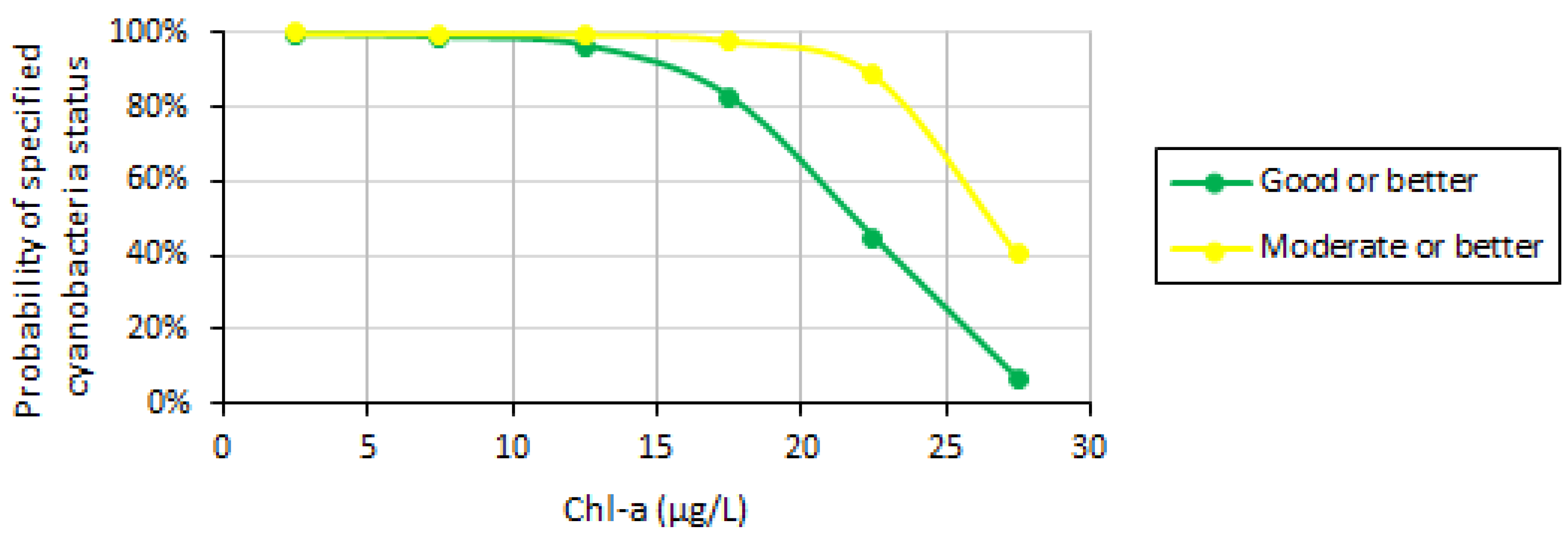
Figure 1. Simplified illustration of the Bayesian network (BN) model for Lake Vansjø, embedded in the conceptual framework of the MARS (Managing Aquatic ecosystems and water Resources under multiple Stress) project. Oval nodes are variables in the BN model; boxes show the sources of data and other information. The BN model has five modules, which can be mapped to the DPSIR framework (Figure 1): (1) Climate and management scenarios (yellow nodes; Drivers); (2) output from the process-based lake model MyLake (blue nodes; Pressures and abiotc States); (3) climatic data (red nodes; Pressures or abiotic States), (4) monitoring data from Lake Vansjø (green nodes; biotic States); and (5) the national classification system for ecological status of lakes (grey nodes; Impacts). The set of arrows pointing to a node represents the conditional probability table for this node.
Water 11 01767 g001
Figure 2. Location and land-use distribution in the Vansjø-Hobøl catchment. The MyLake model is evaluated at the Vanemfjorden station (open circle), while Kure is the main river monitoring site. A black arrow indicates the outlet of the lakes to the Oslo fjord. (After [27]).
Water 11 01767 g002
Figure 3. Exploratory analysis of candidate variables for the Bayesian network model. The main response variable of interest is cyanobacteria. New predictor variables compared to [17] are the meteorological variables air temperature, wind speed, and precipitation. The lower left panel displays the correlation coefficient (r) of each variable pair, with font size proportional to r. The upper right panel displays the scatter plot with a smoothed regression curve.
Water 11 01767 g003
Figure 4. Regression tree analysis showing significant changes in cyanobacteria abundance along each of the explanatory variables (a) Lake temperature (°C) and (b) Wind speed (m/s). The numbers below each branch display the deviance and the number of observations.
Water 11 01767 g004
Figure 5. Illustration of the cumulative link model with three response categories for the status of cyanobacteria (High-Good, Moderate, or Poor-Bad), given lake temperature >19 °C and wind speed <3.4 m/s. The green curve shows the probability of cyanobacteria status being Good or better (CyanoMax < 1000 µg/L); the yellow curve shows the cumulative probability of status Moderate or better (CyanoMax < 2000 µg/L).
Water 11 01767 g005
Figure 6. Examples of conditional probability tables (CPTs) parameterized by different approaches. (a) CPT based on counts of data: Chl-a conditionally on Scenario (MARS storyline, see Table 4) and Month. (b) CPT based on a statistical model: for cyanobacteria conditionally on temperature, wind, and Chl-a. (c) CPT based on a combination rule: status of phytoplankton conditionally on Chl-a and cyanobacteria. The color code is used to visualize the gradient of probabilities from 0% (green) to 100% (red), which can be particularly helpful when the probability tables are parameterized by counts (a).
Water 11 01767 g006
Figure 7. BN model runs for two explorative scenarios (see Table 5): (a) warm and windy weather, and (b) warm and calm weather; both with intermediate Chl-a concentration (15–20 µg/L), for July. The change from windy to calm weather results in increased probability of cyanobacteria abundance exceeding 1000 µg/L (from 0% to 17% probability). State names: "x0__3.4" represents the interval 0–3.4. Status codes: HG = High-Good; M = Moderate, PB = Poor-Bad. Note: the bar colors are automatically selected by the software (GeNIe) and do not represent any color code.
Water 11 01767 g007
Figure 8. Examples of results from exploratory scenarios of weather conditions (Table 5) and Chl-a concentrations. The two weather scenarios Warm & Windy (a,b) and Warm & Calm (c,d) are combined with three intervals of Chl-a concentration: 0–10.5 µg/L (High-Good status), 10.5–20 µg/L (Moderate status), and >20 µg/L (Poor-Bad status). The left panel (a,c) shows the probability distribution of cyanobacteria status; the right panel (b,d) shows the probability of phytoplankton status, which combines Chl-a status and cyanobacteria status (cf. the combination rule in Figure 6c). Note that the results shown in the upper panel are also representative for the two weather scenarios Cold & Calm and Cold & Windy.
Water 11 01767 g008
Figure 9. BN model runs for two MARS storylines (see Table 2) for the time horizon 2060 (2050–2070): (a) Consensus World and (b) Techno World. Note that the worsening of lake status (lower probability of High-Good) in the Techno World storyline is mainly driven by nutrient concentrations rather than climatic variables. For more details, see Figure 7.
Water 11 01767 g009
Figure 10. Predicted probability distributions for selected nodes of the BN model of Lake Vansjø: (a) Wind speed, (b) Cyanobacteria status, (c) Lake temperature, (d) Chl-a status, (e) Phytoplankton status, (f) Total P and (g) Lake status (ordered according to the nodes’ positions in Figure 1). Projections for the future climate scenarios and storylines using the IPSL climate model are shown, for the 20-year period 2050–2070 (months May–October). Color codes: Temperature: blue = Cold (<19 °C), red = Warm (≥19 °C). Wind speed: blue = calm (<3.4 m/s), red = windy (≥3.4 m/s). Status nodes: green = High-Good, yellow = Moderate, brown = Poor-Bad. Cyanobacteria concentration: green = <1000, yellow = 1000−2000, brown = >2000 (μg/L). Future scenarios and storylines: BL = extended baseline, 4.5 = climate scenario, RCP4.5, 8.5 = climate scenario RCP8.5, CW = Consensus World, FW = Fragmented World, TW = Techno World.
Water 11 01767 g010
Table 1. Boundaries of status classes (all in μg/L) for biological and chemical elements included in the BN model, according to the Norwegian classification system, for lakes of type L-N8a (large, lowland, moderately calcareous, humic) [36].
VariableGood/ModerateModerate/Poor
Chl-a10.520
CyanoMax10002000
Total P2039
Table 2. Downscaling of the MARS storylines focusing on agricultural and water-related development for the Lake Vansjø catchment (Morsa). All storylines assume an extension of the growing season by two months. RCP: representative concentration pathway. WWTPs: wastewater treatment plants. After [23].
StorylineClimate ScenarioAgricultural DevelopmentWater-Related Development
Consensus WorldRCP4.510% of grassland converted to forest;
30% shift from vegetables and crops to unfertilized grasslands;
50% decrease in fertilization;
50% decrease in erosion
50% decrease in effluent from scattered dwellings and WWTPs
Fragmented World 1RCP8.55% of forest converted to grassland;
30% of grassland converted to arable land;
15% increase in fertilization;
15% increase in erosion
25% increase in effluent from scattered dwellings and WWTPs
Techno World 1RCP8.510% of forest areas converted to grassland;
60% of grassland converted to arable land;
30% increase in fertilization;
30% increase in erosion;
40% increase in effluent from scattered dwellings and WWTPs
1 Fragmented World and Techno World have different interpretations in Couture et al. [27] and Mack et al. [23]. We follow the labelling used by Couture et al. [27].
Table 3. Model comparison of ordinal regression models with cyanobacteria as response variable and candidate predictor variables Chl-a (continuous), Lake temperature (binary), and Wind speed (binary). AIC: Akaike’s Information Criterion. Lower AIC values indicate a better model.
Model No.Explanatory VariablesNumber of Obs.AIC
1Chl-a10791.54
2Lake temperature90117.9
3Wind speed9081.4
4Chl-a + Lake temperature9070.7
5Chl-a + Wind speed7755.9
6Chl-a + Lake temperature + Wind speed7356.4
Table 4. Overview of nodes in the Bayesian network model. More details on the states are described by [17]. For “Classification system”, see Table 1. For “MARS storylines”, see Table 2.
Node GroupNode LabelState TypesNo. of StatesSource of Probability Table
ScenariosScenario no.Numbers25(Root node)
Climate scenarioCategories3MARS storylines
Agriculture scenarioCategories4MARS storylines
Domestic wastewater scenarioCategories4MARS storylines
Period
(time horizon)
Numbers3MARS storylines
MonthCategories6(Root node)
ClimateWind speedIntervals (unit: m/s)2Count of data (simulated)
Process-based lake modelLake temperatureIntervals (unit: °C) 2Count of data (simulated)
Chl-aIntervals (unit: µg/L)6Count of data (simulated)
Total PIntervals (unit: µg/L)6Count of data (simulated)
Biological monitoring dataCyanobacteriaIntervals (unit: µg/L)3Statistical model
CyanoMaxIntervals (unit: µg/L)3Classification system
Ecological statusStatus CyanobacteriaOrdered categories3Classification system
Status Chl-aOrdered categories3Classification system
Status PhytoplanktonOrdered categories3Classification system
Status Total POrdered categories3Classification system
Status of lakeOrdered categories3Classification system
Table 5. Explorative what-if scenarios for cyanobacteria defined by weather conditions.
VariableLow State NameLow IntervalHigh State Name High Interval
Wind speedCalm<3.4 m/sWindy>3.4 m/s
Lake temperatureCold<19 °CWarm>19 °C
Table 6. Overview of process-based model predictions for selected MARS scenarios and storylines. For each scenario, the table shows mean values (and standard deviations) of variables predicted by climate model IPSL (wind) or lake model MyLake (lake temperature, Total P, and Chl-a) for months May–October, time horizons 2030 and 2060 respectively. Scenarios codes: BL = extended baseline, 4.5 = climate scenario RCP4.5, 8.5 = climate scenario RCP8.5, CW = Consensus World, FW = Fragmented World, TW = Techno World (see Table 2).
ScenarioClimateAgriculture ScenarioWastewater ScenarioWind (m/s)Lake Temperature (°C)Total P (µg/L)Chl-a (µg/L)
CodeName20302060203020602030206020302060
BLExtended baselineCurrentCurrent Current 2.16 (0.48)2.17 (0.55)14.8 (4.8)14.9 (4.7)16.7 (6.0)14.1 (5.6)8.3 (4.5)6.3 (3.7)
4.5RCP4.5RCP4.5Current Current 2.13 (0.54)2.11 (0.53)17.4 (4.7)18.4 (4.5)17.6 (5.3)15.9 (5.2)8.7 (4.0)7.2 (3.5)
8.5RCP8.5RCP8.5Current Current 2.08 (0.46)2.05 (0.51)17.6 (4.9)19.2 (4.4)17.1 (5.3)16.0 (5.0)8.6 (4.1)7.3 (3.5)
CWConsensus WorldRCP4.5EnvironmentalStable2.13 (0.54)2.11 (0.53)17.4 (4.7)18.4 (4.5)14.1 (4.1)12.4 (3.5)7.6 (3.7)6.2 (3.0)
FWFragmented WorldRCP8.5IntermediateIntermediate2.08 (0.46)2.05 (0.51)17.6 (4.9)19.2 (4.4)19.1 (6.2)18.3 (6.1)9.2 (4.3)8.0 (3.9)
TWTechno WorldIntensiveIncrease21.4 (7.3)21.1 (7.5)9.9 (4.7)9.0 (4.3)

