Improving the Accuracy of Hydrodynamic Simulations in Data Scarce Environments Using Bayesian Model Averaging: A Case Study of the Inner Niger Delta, Mali, West Africa

Abstract

In this paper, the study area was the Inner Niger Delta (IND) in Mali, West Africa. The IND is threatened by climate change, increasing irrigation, and dam operations. 2D hydrodynamic modelling was used to simulate water levels, discharge, and inundation extent in the IND. Three different digital elevation models (DEM) (SRTM, MERIT, and a DEM derived from satellite images were used as a source of elevation data. Six different models were created, with different sources of elevation data and different downstream boundary conditions. Given that the performance of the models varies according to the location in the IND, the variable under consideration and the performance criteria, Bayesian Model Averaging (BMA) was used to assess the relative performance of each of the six models. The BMA weights, along with deterministic performance measures, such as the Nash Sutcliffe coefficient (NS) and the Pearson’s correlation coefficient (r), provide quantitative evidence as to which model is the best when simulating a particular hydraulic variable at a particular location. After the models were combined with BMA, both discharge and water levels could be simulated with reasonable precision (NS > 0.8). The results of this work can contribute to the more efficient management of water resources in the IND.

1. Introduction

The Inner Niger Delta (IND) is the second-largest wetland in Africa, and its maximum inundated area can exceed 30,000 km² during wet years [1]. Its main water sources are the Niger and Bani Rivers, which enter the study area at Ké-Macina and Sofara, respectively, flowing through the Delta over several hundred kilometers, before both exit at Diré (Figure 1). The maximum inundation area shrinks to around 10,000 km² in dry years [2] under the combined impacts of climate variability, irrigation withdrawals, and dam operation. The IND faces many environmental challenges due to upstream water interventions on the river system, as well as high precipitation variability.

The IND is considered as a hub of human activities, including agriculture, fishing, transport, and tourism. The Delta plays an important role in promoting sustainable development for food security, water management, and the environment. Some upstream dams and irrigation structures are already in place, while more are at the planning stage. The infrastructures aim to increase economic development and food security. However, damming a river often implies a transfer of benefits from the downstream to the upstream regions. Thus, damming the main course or branches of the Niger River can impact on food security, ecology, and the environment as a whole by altering flow and inundation patterns. The operation of existing dams, such as Sélingué, Markala, and Talo has already modified flow patterns in the Delta, and planned dams, such as Fomi and Djenné, may exacerbate the changes. Figure 2 shows the location of existing and planned dams/reservoirs upstream of IND. Zwarts and Frerotte [1] have shown that on average, 9% of the total flood extent area has been lost due to the effects of the Selingue and Markala dams. Liersch et al. [3] anticipated an average reduction of 24% flood extent compared to the natural condition due to the combined effect of existing and planned water infrastructures in the watershed. The situation may get worse due to increased evaporation as a result of global warming [4]. However, changes in precipitation are uncertain [5] where some models project a wetter, and others a drier future in the Upper Niger basin [6]. A lower flow rate, in combination with a smaller flood plain, will most probably affect crop yields, fisheries, livestock, biodiversity, and environmental flow. To understand the possible impacts of these future changes on ecosystems and livelihoods, a realistic simulation of water levels, flow velocity, and inundations are required.

Concerns about the hydrologic regime alterations in the watershed have triggered interest in ecosystem services and environmental health, especially in the IND area. The evaluation of ecosystem health requires the knowledge of relevant hydraulics parameters under altered flow scenarios. Such knowledge can only be achieved using hydrodynamic modelling. Unfortunately, previous attempts to develop a hydrodynamic model of the IND were only partially successful. For instance, Neal et al. [7] applied LISFLOOD-FP [8], a raster-based sub-grid model, but model results were affected by the low-resolution (about 1 km) structured grid and simplified assumptions about the solution of the St. Venant equation. Dadson et al. [9] applied a one-dimensional model with 25 km grids, and presented the inundation as a fraction of the cells which did not show the variability of inundation. Haag [10] applied the D-Flow FM [11,12], a shallow-water solver based on the finite-volume method on an unstructured grid to study the flood in the delta, and ended up having an imperfect simulation of water level, where inundation resulted from poor calibration efforts.

This study is an attempt to develop a working hydrodynamic model for the IND in support of ecosystems studies in the area. The modelling was done using TELEMAC 2D [13], a finite-element computer program suite that solves shallow-water equations using the finite element method. Given the lack of accurate digital elevation models of the study area, two global digital elevation models were considered: the Shuttle Radar Topography Mission (SRTM) [14], and the Multi-Error-Removed Improved-Terrain (MERIT DEM) [15]. However, the elevation accuracy of the DEMs makes their use in hydrodynamic modelling challenging. Rodriguez et al. [16] reported an elevation error (standard deviation) of about 4.68 m of SRTM DEM in Africa. Yamazaki et al. [15] reported a relative vertical height error of about 2 m of MERIT DEM for 58% of the land mapped by the DEM. A third DEM was therefore derived using the waterline method [17,18,19].

Downstream boundary conditions were imposed by prescribing rating curves either in the form of discharge as a function of water level or water level as a function of discharge. Inflows in the domain were a combination of measurements and simulations using a Soil Water Assessment Tools (SWAT) hydrological model [20] of the Upper Niger Basin. The combination of all available DEMs and downstream conditions led to a total of six models with different performances in simulating discharges, water levels, and inundation extents. Bayesian Model Averaging (BMA) [21] was used to combine the outputs of these six models to get improved results and identify the best individual models that could be used to simulate water levels and discharges with relatively high performance.

The paper is organized as follows: Section 1 contains the background and objective of the study; Section 2 presents the materials and methods, which includes available data, topographic data derivation, river network, bathymetric data, floodplain friction, adjustment of the elevation of SRTM and MERIT DEM, model setup, model calibration, and the theory of BMA; Section 3 deals with calibration results, BMA prediction, validation results, inundation extent, and performance of global DEMs; and finally, some concluding remarks complete the study.

2. Materials and Methods

2.1. Available Data

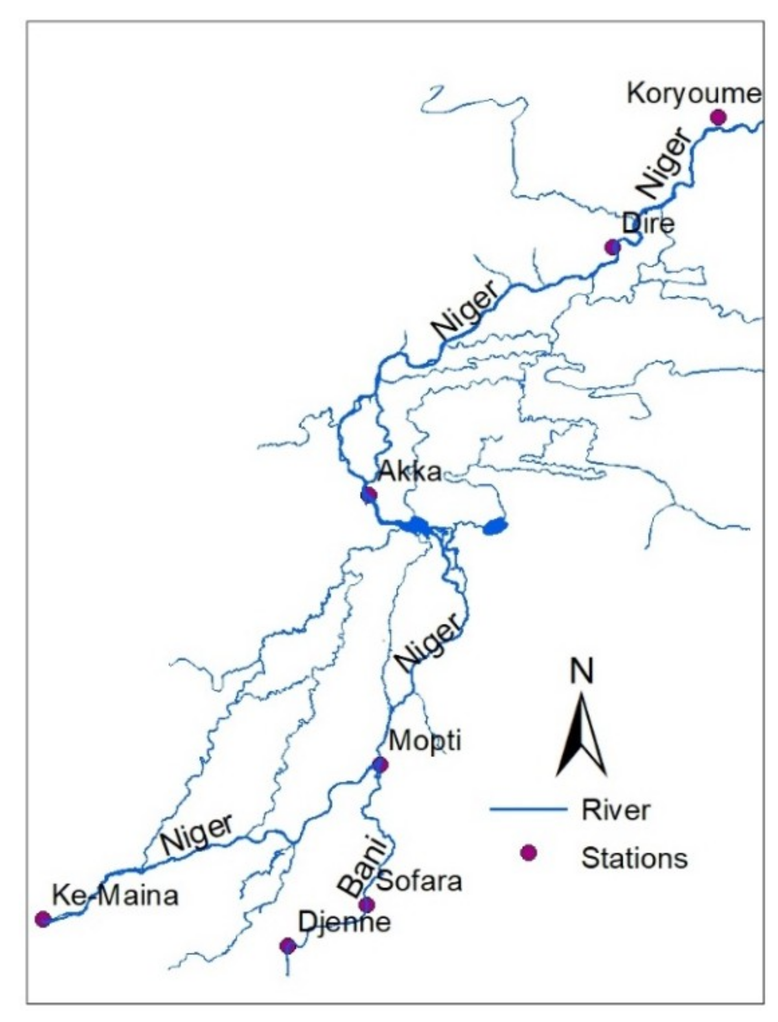
2.1.1. Discharge and Water Level

Water levels and discharge at Ké-Macina, Sofara, Mopti, Akka, and Diré, as well as a rating curve at Diré were obtained from the Malian hydrometric services (Direction Nationale de l’Hydraulique, DNH). Water level data have been referenced to Institut national de l’information’s (IGN) datum. Water entered into the study area at KeMacina and Sofara through the Niger and Bani rivers, respectively. Mopti is located downstream of the confluence of the Bani and Niger rivers. Akka is situated almost at the middle of the study area, along the Niger River. Water drains the system at Dire station.

2.1.2. Topographic Data Sources

The SRTM DEM has been available at a resolution of one arc-second (about 30 m) since 2014. It is a widely used DEM: Biancamaria et al., Schumann et al., and Neal et al. [7,22,23] used SRTM gridded data for hydraulic modelling of the Ob in western Siberia, the Scioto River in the eastern U.S., and the Niger River (Inner Niger Delta) in Mali, respectively. The SRTM elevation data used in this study were downloaded from https://earthexplorer.usgs.gov/.

The MERIT DEM is available at three arc-sec resolutions (about 90 m), and was derived from SRTM and AW3D-30 m [24] by removing multiple error components, such as absolute bias, stripe noise, speckle noise, and tree height bias [15]. The MERIT DEM was used by Hawker et al. and Archer et al. [25,26] for the flood modelling study of the Ba catchment, Fiji. The MERIT DEM was downloaded from http://hydro.iis.u-tokyo.ac.jp/~yamadai/MERIT_DEM/.

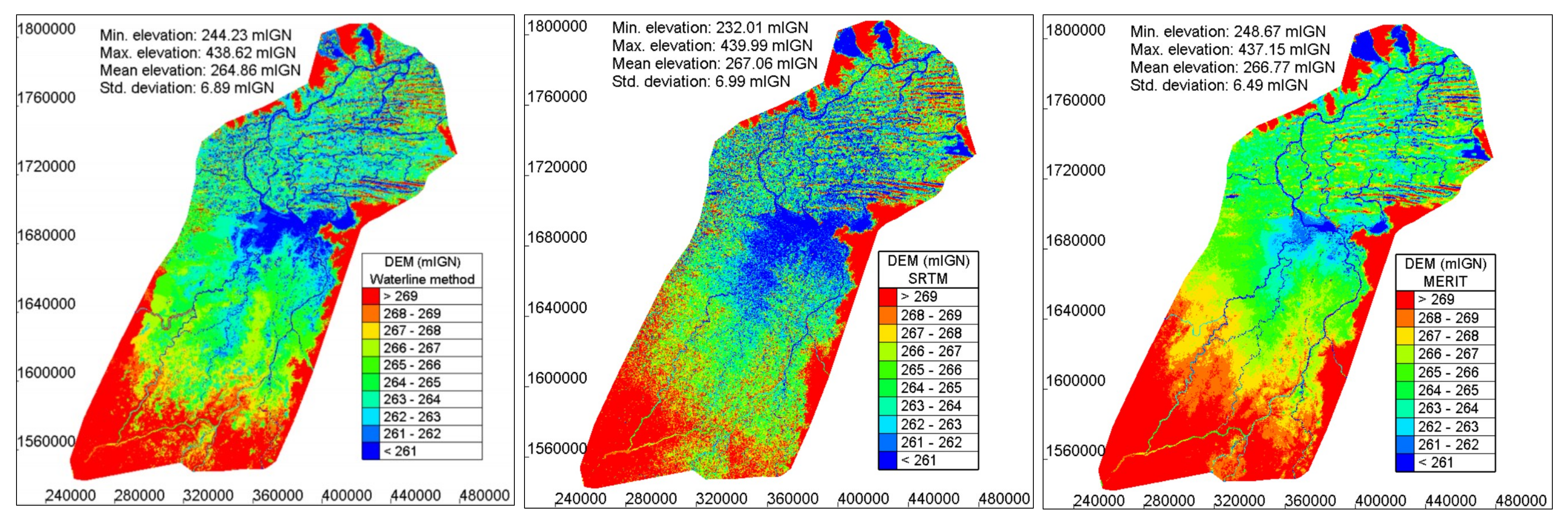
2.1.3. DEM Derivation Using the Waterline Method

An additional DEM was developed using the waterline method from the combined uses of the water extent map derived from Landsat satellite images by Zwart et al. [2] and water level data collected on particular dates. The waterline method involves determining the horizontal position of the land–water boundary from a time series of remotely sensed images taken during different periods, and then superimposing on this boundary the heights relative to a datum.

The procedure is as follows:

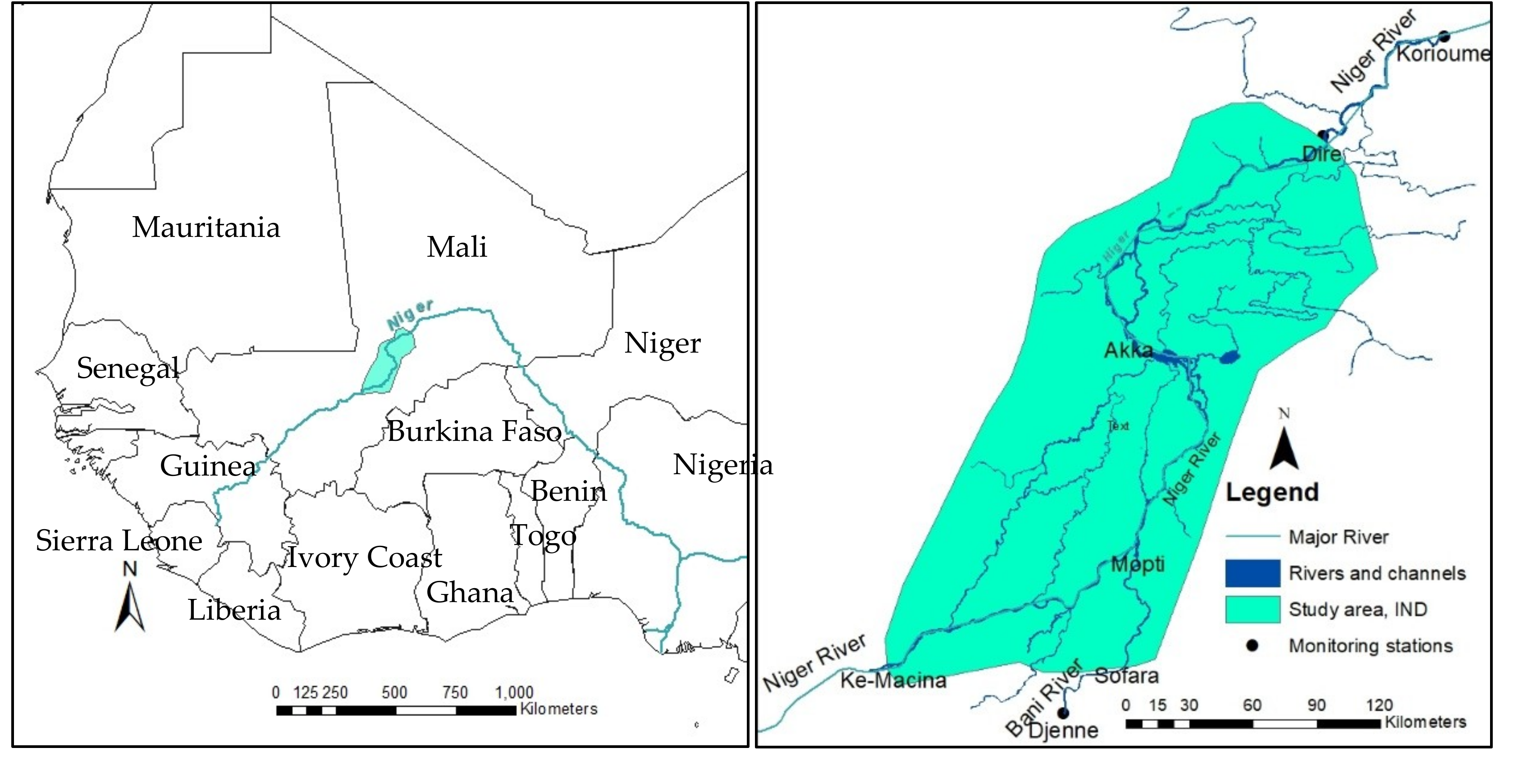
• Seven inundation extent polygons derived from Landsat satellite images by Zwarts et al. [2] for dates 5 July 1985, 10 June 2001, 8 August 1984, 28 July 2001, 25 October 1984, 16 October 2001, and 28 November 1999 were selected to represent the range of possible water elevations in the Inner Delta.
• For each of the seven flood inundation maps, water levels at Ké-Macina, Mopti, Akka, and Diré were used to calculate the slope of the water surface along principal flow paths between Ké-Macina and Akka, between Mopti and Akka, and between Akka and Diré. In the absence of additional information, it was further assumed that the water level variation between any two stations is linear.
• A series of orthogonal lines were drawn at 30 m intervals along principal flow paths.
• It was assumed that water levels along these lines are constant. Therefore, an elevation value could be set at the intersection points between water extent polygon and the orthogonal lines.
• At the end of the process, an altitude was estimated for each point within the flood extent polygons.
• Areas outside the larger polygon were populated using SRTM elevation data.
• GIS was used to interpolate the elevation data inside the study area.

The mean elevation of the Waterline DEM, SRTM, and MERIT DEM were 264.86 m, 267.06 m, and 266.77 m, respectively (Figure 3).

2.1.4. Satellite Imagery

This study makes use of the water extent maps derived from Landsat images by Zwarts et al. [2]. Zwarts et al. [2] processed Landsat 5 TM images captured on 24 different dates spanning from 1984 to 2003, and derived 24 water extent maps for the study area. The images provide evidence of the water extents of inundation areas, along with known water levels at Mopti, Akka, and Diré. The inundation extent obtained from the images on 28 July 2001 and 16 October 2001 are shown in Figure 4.

To validate the simulated inundation, a series of Moderate Resolution Imaging Spectroradiometer (MODIS) images were processed to derive the inundation extent. A summary of the satellite data usage is given in

Table 1. Satellite images used in the study.

Image Source/Name	Satellite	Path/Row	Purpose	Date Captured	Resolution
Several images from Zwart et al. [2]	Landsat 5 TM	197/49 and 197/50	Model setup, Calibration	1984 to 2001	30 m
MOD09A1.A2008241 MOD09A1.A2008281 MOD09A1.A2009017	MODIS	-	Model validation	28 August 2008 7 October 2008 17 January 2009	500 m

.

We used two spectral indices to separate water pixels from non-water pixels. The indices are the Modified Normalized Difference Water Index (MNDWI) [27] and the Normalized Difference Moisture Index (NDMI) [28].

MNDWI and NDMI indexes are expressed as follows:

$$\mathrm{MNDWI}=\frac{\mathrm{Green}-\mathrm{MIR}}{\mathrm{Green}+\mathrm{MIR}}$$

(1)

$$\mathrm{MDMI}=\frac{\mathrm{NIR}-\mathrm{MIR}}{\mathrm{NIR}+\mathrm{MIR}}$$

(2)

For MODIS images, Green, NIR, and MIR represent reflectance from Band 4 (545 nm–565 nm), Band 2 (841 nm to 876 nm), and Band 6 (1628 nm to 1652 nm), respectively. The study makes use of the finding by Ogilvie et al. [29] on the threshold value of NDMI and MNDWI. They analyzed MODIS images to study the spatial and temporal dynamics of floods across the Niger Inner Delta over the period of 2000–2011. Water was classified when the pixel had a threshold value of 0.15 for NDMI, and for the MNDWI, classifying pixels above the threshold of −0.34 was considered a flooded area.

2.2. River Network

The river network was derived from the inundation extent map derived from a Landsat image on 8 July 1985 by Zwarts et al. [2]. Only major rivers and channels were extracted. Small channels, especially at the northern part of the delta, could not be taken into consideration due to their haphazard geometry and complex meandering. Figure 5 shows the delineated river network used in the model.

2.3. Channel Geometry

The bed elevation of river sections at Ké-Macina, Mopti, Akka, and Diré was approximated using hydraulic geometry equations proposed by Leopold and Maddock [30]. Hydraulic geometry relationships are a series of power laws that relate river width (w), depth (d), and velocity (v) to discharge. These functions are:

$$w=a{Q}^b$$

(3)

$$d=c{Q}^f$$

(4)

$$v=k{Q}^m$$

(5)

Here, a, c, and k are coefficients, and b, f, and m are exponents with $b+f+m=1, \mathrm{and}$

$$a\times c\times k=1.$$

Empirical values of the hydraulic geometry coefficients and exponents derived by Hey and Thorne [31] for Gravel-Bed Rivers in Britain were used in this study. Hey and Thorne [31] found that a = 3.67, b = 0.45, c = 0.33, and f = 0.35 were a fair representation of hydraulic geometry. The same coefficients were used by Neal et al. [7] in the IND.

Leopold [32] suggested taking the bankfull discharge for the analysis, as it is related to channel morphology. The bankfull discharge is often assumed to be the discharge, with a return period of about 1.5 years.

Table 2. Bed elevation of the Niger River at Ke-Macina, Mopti, Akka, and Dire.

Monitoring Stations	Bankfull Discharge (m3/s)	Bankfull Stage (mIGN)	Bankfull Depth (m)	Bed Elevation (mIGN)
KeMacina	3518.00	274.31	5.81	268.50
Mopti	2340.00	266.42	5.04	261.38
Akka	1816.00	262.81	4.61	258.20
Dire	1760.00	261.45	4.56	256.89

shows the river bed elevation at KeMacina, Mopti, Akka, and Dire. Elevations of other points in between the sections were calculated assuming a linear variation along the longitudinal direction.

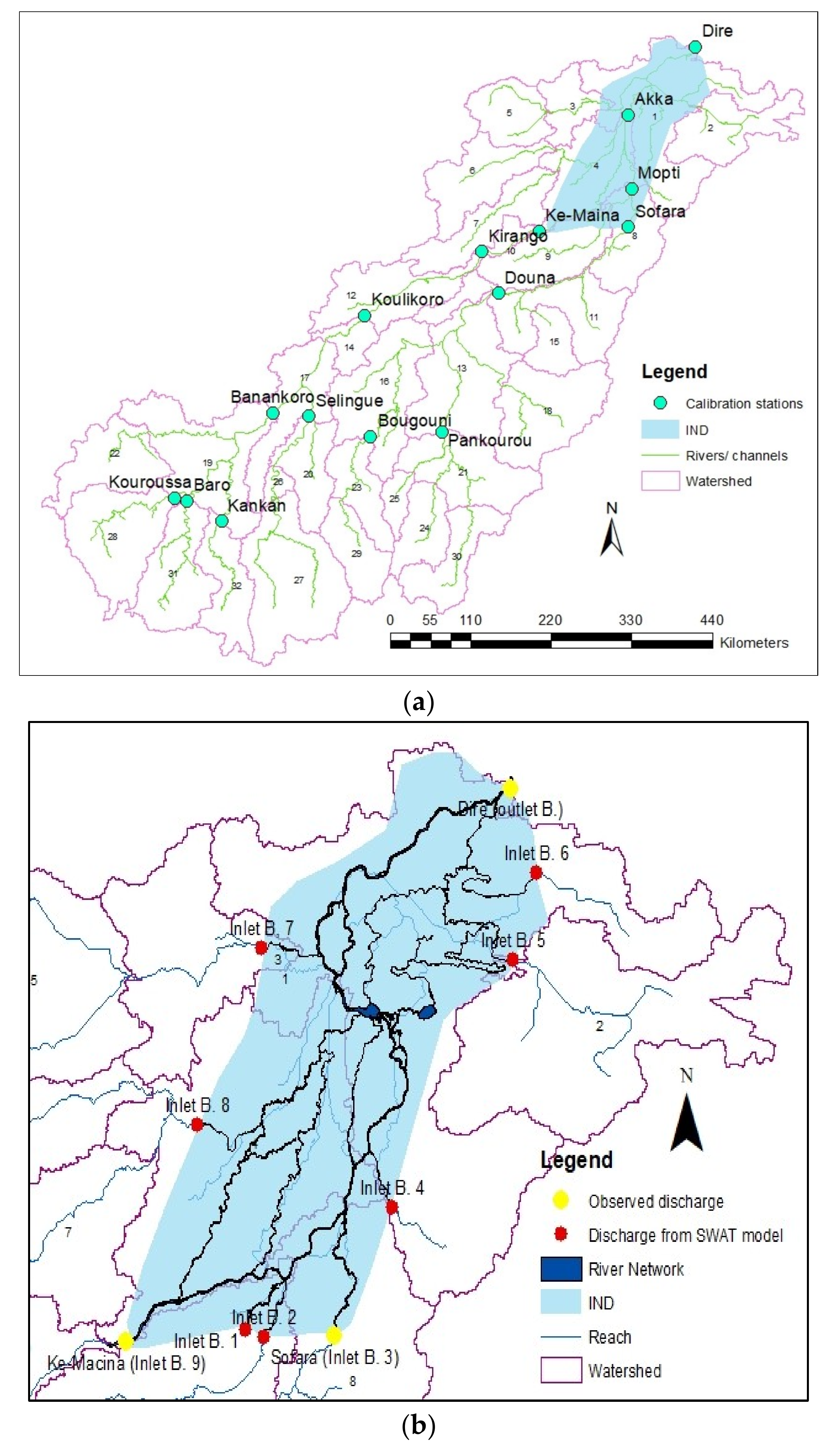
2.4. Estimation of Inflow at Ungauged Inlets

Observed streamflow time series were available only at two inlets of the hydrodynamic model domain, namely Ke-Macina and Sofara. Streamflow at the seven other inlets was generated by local precipitation that generate ephemeral streams which ultimately end up in the IND. These ungauged inflows were estimated using a SWAT model of the upper Niger and Bani Rivers basins developed in a previous project [33]. SWAT is a process-based and spatially semi-distributed hydrological model. In the SWAT model, the whole watershed is divided into multiple sub-basins, and each sub-basin is divided into several Hydrological Responsible Units (HRUs) that consist of unique homogeneous combinations of soil, land use, and topographic features in each sub-basin [34]. The hydrological cycle simulated by the SWAT model is based on the water balance equation [35]:

$$S{W}_t=S{W}_0+{\displaystyle \sum }_{i=1}^{i=0}\left(R_{day}-Q_{surf}-E_a-W_{perc}-Q_{gw}\right)$$

(6)

where $S{W}_t$, $S{W}_0$ are the final and initial soil water content (mm/d), respectively; t is the time (day); $R_{day}$ is the precipitation(mm/d); $Q_{surf}$ is the runoff (mm/d); $E_a$ is the evapotranspiration (mm/d); $W_{perc}$ is the percolation (mm/d); and $Q_{gw}$ is the return flow (mm/d). The SWAT model implements multiple options for the description of hydrological processes, such as the Soil Conservation Service (SCS) curve number method [36] for runoff calculation and the Penman-Monteith [37] method for the estimation of potential evapotranspiration. The details on SWAT modelling tools can be found from Arnold et al., [20], Arnold et al. [33], and Neitsch et al. [35].

The SWAT model of the UNB contains 32 sub-watersheds (Figure 6a). The model was calibrated and validated using streamflow from 14 hydrometric stations listed in

Table 3. Calibration and validation performance of the Soil Water Assessment Tools (SWAT) model.

Monitoring Station	Latitude	Longitude	NS at Calibration	NS at Validation
Kankan	10.38	−9.31	0.65	0.8
Baro	10.51	−9.72	0.68	0.73
Kouroussa	10.64	−9.88	0.68	0.78
Banankoro	11.68	−8.67	0.86	0.9
Sélingué	11.64	−8.24	0.45	0.64
Koulikoro	12.85	−7.56	0.87	0.93
Kirango	13.69	−6.08	0.86	0.82
Ké-Macina	13.95	−5.36	0.9	0.91
Bougouni	11.39	−7.45	0.77	0.78
Pankourou	11.44	−6.58	0.74	0.6
Douna	13.21	−5.9	0.79	0.9
Mopti	14.49	−4.21	0.8	0.78
Akka	15.4	−4.24	0.87	0.84
Diré	16.27	−3.39	0.9	0.75

, along with the calibration and validation performance. The performance criteria used in the calibration and validation process is NS. Sensitivity analysis was performed to select the parameters to use for calibration: CN2 (SCS runoff curve number for moisture condition II), RCHRG_DP (Deep aquifer percolation fraction), and RES_K (Hydraulic conductivity of the reservoir bottom, mm/hr) which were tuned during calibration. The Sequential Uncertainty Fitting program, SUFI-2 [38] was used for calibration purposes. A detailed description of the model used in this study can be found in Seidou [33] and Maiga [39].

The calibrated SWAT model was forced with observed climate data, and the discharge from surrounding watersheds was assumed to enter the area where the main channel crosses the boundary of the study area (red dots in Figure 6b). Yellow dots in Figure 6b indicates observed discharge stations. The formulas used to calculate inflows into the hydrodynamic model domain from the SWAT model outputs are provided in

Table 4. Inflows into the hydrodynamic model domain from the SWAT model outputs.

Inlet Point Location	SWAT Model Subbasin(s)	Remarks
Inlet boundary 1 (Inlet B. 1)	Watershed 9	60% of the outflow of watershed 9
Inlet boundary 2 (Inlet B. 2)	Watershed 9	40% of the outflow of watershed 9
Inlet boundary 4 (Inlet B. 4)	Watershed 1	0.2126 * (Inflow of watershed 1-Outflow of watershed 1)
Inlet boundary 5 (Inlet B. 5)	Watershed 2	Outflow of watershed 2
Inlet boundary 6 (Inlet B. 6)	Watershed 1	0.125 * (Inflow of watershed 1-Outflow of watershed 1)
Inlet boundary 7 (Inlet B. 7)	Watershed 3	Outflow of watershed 3
Inlet boundary 8 (Inlet B. 8)	Watershed 6 and watershed 7	Outflow of watershed 6 + Outflow of watershed 7

* 0.2126 and 0.125 are the fractions of watershed 1 that lie outside the study area in each case.

.

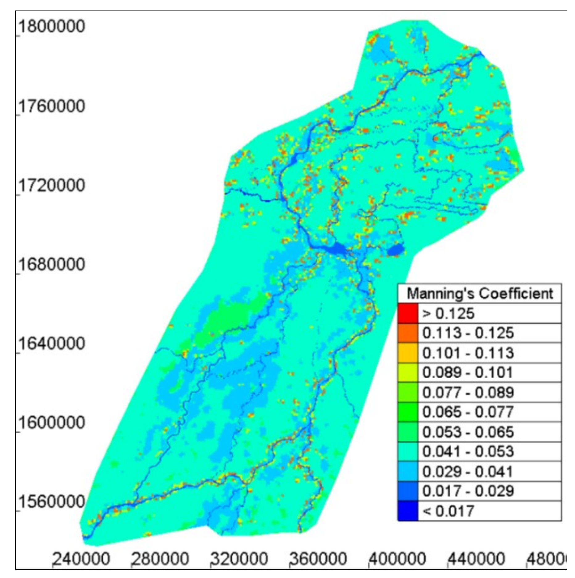
2.5. Floodplain Friction

The Manning roughness coefficient was derived from the USGS Global Land Cover Characterization [40] database following Asante et al. [41]. Figure 7 shows the distributed Manning’s roughness coefficient at the IND.

2.6. Hydrodynamic Model Setup

The hydrodynamic modelling was performed using TELEMAC 2D, a hydrodynamic model used worldwide. TELEMAC-2D solves the depth-integrated Shallow Water Equations (SWEs) using the finite element method on an irregular mesh.

In TELEMAC 2D, the SWE’s are solved using a fractional step method [42], whose main principle is that the hyperbolic and parabolic parts of the SWE’s should be treated separately. The solution comprises two steps: a solution of advection terms, and the solution of the propagation, diffusion, and source terms. Several schemes are available for the advection step, where the Method of Characteristics has been applied to solve the advection of u and v. The Streamline Upwind Petrov-Galerkin (SPUG) method [43] has been applied to solve the advection of h in the continuity equation. Variational formulations and space discretization transform the continuous equations into a linear triangular element, where the dependent variables u, v, and h are expanded using equal order interpolation functions. In the second step, the propagation, diffusion, and source terms are coupled through an implicit time scheme, and the resulting linear system is solved with a variant of the conjugate gradient method [44].

2.6.1. Mesh Generation

The entire domain was discretized using a system of irregular triangular elements. In the channel mesher, the rivers and channels were discretized separately, and in the combined mesher, the river and flood plain were joined together to form a combined mesh. The combined mesh has 220,289 nodes and 438,716 elements. The smallest length of the elements is about 50 m, and maximum length is about 844 m.

2.6.2. Model Boundary Conditions

The model has ten liquid boundaries. Nine of the liquid boundaries are inlets, while the last one is an outlet boundary. The location of liquid boundaries is shown in Figure 6b. Time-varying discharges were used to prescribe flows at the inlet boundaries. Among the nine inlets, two are fed with the measurement, and seven comes from the output of a SWAT model. The downstream boundary is prescribed with two types of rating (stage-discharge) curves, where the Type (1) rating curve is in the form of water level as a function of discharge, and the Type (2) rating curve is in the form of discharge as a function of water level. We used a relaxation parameter to the Type 1 rating curve to possibly obtain a stable simulation of water level and discharge free from oscillation, as suggested by Hervouet [13]. Relaxation to the rating curve gives rise to the possibility of a smoothly varying boundary condition, which may otherwise trigger instabilities [13].

Rainfall was not included in the hydrodynamic model, because local rainfall has some effect on IND flood magnitude. The IND is in a semi-arid area, and most of the water flowing in it comes from a very humid region in Guinea, 600–900 km upstream. The headwaters’ annual rainfall can go up to 1750 mm. However, in IND, average annual rainfall varies between 200 mm/yr at the downstream and 500 mm/yr at the upstream [2]. We did account for precipitation and evaporation on the watershed through the SWAT model, but chose not to include precipitation directly on the water body. Zwarts [45] found that local rainfall was too limited to influence the flood height in IND.

The authors acknowledge that constant evaporation has a lot of limitations, but the estimation of evaporation in the IND is an ongoing debate, with multiple papers published on the topic, and rather diverging estimates. Evaporation varies between 160 and 240 mm per month, with an average of 200 mm per month [2]. Ogilvie et al. [29] found evaporation rates were between 4 mm/day and 7 mm/day over the years 2008–2009.

Given the huge uncertainty in the estimated evaporation and the fact that our main purpose was flood wave propagation, we believe that the choice of constant evaporation had little impact on the results. The authors are considering the inclusion of dynamic precipitation and evaporation in the model that involves modifications of the TELEMAC 2D routines.

2.6.3. Initial Conditions

An introductory simulation was performed with prescribed constant discharges at each inlet, as well as a constant prescribed elevation at the outlet boundary to obtain the initial condition for subsequent runs. The simulation time step was set as 60 sec. It was selected in such a way so that it would not produce any instability on the simulation. It is to be noted that the courant number gives the impression of the stability of the model to perform the calculation. The courant number of the simulation was kept below 4. Manning’s friction coefficient, as discussed in the previous section, was assigned to the nodes. The Manning coefficient at the floodplain was constant during simulation. However, the Manning’s coefficient at the river channel was considered variable, and tuned during calibration.

2.6.4. Model Configurations

Given that three elevation data sets were available and that there were two possibilities for downstream boundary conditions to be set (by prescribing a rating curve in one of the following forms: discharge as a function of water level—type 1 or water level as a function of discharge—type 2), we obtained total of six different hydrodynamic models (

Table 5. Configuration of the six models.

Model Number	Elevation Data	Downstream Boundary Condition
Model 1	Merit DEM	Rating curve in the form of water level as a function of discharge, R = 0.02
Model 2	Merit DEM	Rating curve in the form of discharge as a function of water level
Model 3	SRTM DEM	Rating curve in the form of water level as a function of discharge, R = 0.02
Model 4	SRTM DEM	Rating curve in the form of discharge as a function of water level
Model 5	Waterline DEM	Rating curve in the form of water level as a function of discharge, R = 0.02
Model 6	Waterline DEM	Rating curve in the form of discharge as a function of water level

). Prescribing Type 1 boundary conditions often leads to resonances or uncontrollable oscillations because of the feedback of the level on the local discharge. To address the issue, the developers of TELEMAC 2D estimated water levels at time t as a weighted average of the water level, corresponding to the discharge prescribed at time t and the water level corresponding to the discharge prescribed at time t − 1. The weight of the water levels corresponding to the prescribed discharge at time t is called the relaxation coefficient (R). The developers of TELEMAC 2D recommend a value of R between 0.01 and 1.0 to smoothly prescribe discharges. In this paper, the value of R has been set to its default value of 0.02.

Ogilvie et al. [29] found that the years 2001–2002 and 2008–2009 experienced relatively few clouds. Our study used these two periods as the calibration and validation period, respectively. MODIS and Landsat images during the months of September–February were considered for extracting water extent, as these months showed fewer clouds than the other months [29]. The periods between 1 July 2001 to 28 February 2002, and from 1 July 2008 to 28 February 2009 were thus chosen for calibration and validation, respectively.

2.7. Calibration

In flood modelling, the roughness coefficient is typically used as a calibration parameter [46]. It is commonly recognized that friction varies in space, and that the precision of simulation can be improved through calibration and the use of effective friction coefficients [47,48]. The model was calibrated by changing the Manning coefficients in the reaches of the Niger river: KeMacina to Mopti (slope = 0.052 m/km), Mopti to Akka (slope = 0.029 m/km), and Akka to Dire (slope = 0.007 m/km). The Manning coefficient in the other reaches was assumed to be constant (0.02). As discussed before, the Manning coefficient of the floodplain was derived from GLCC. The calibration period of the model was chosen as July 2001–February 2002. The simulation results were evaluated by Pearson’s correlation coefficient (r) and Nash-Sutcliffe coefficients (NS) at Akka and Mopti. Pearson’s correlation coefficient (r) and Nash-Sutcliffe coefficients (NS) are described in the following equations:

$$r=\frac{{{\displaystyle \sum }}_{i=1}^n\left(x_i-\overline{x}\right)\left(y_i-\overline{y}\right)}{\sqrt{{{\displaystyle \sum }}_{i=1}^n{\left(x_i-\overline{x}\right)}^2}\sqrt{{{\displaystyle \sum }}_{i=1}^n{\left(y_i-\overline{y}\right)}^2}}$$

(7)

$$NS=1-\frac{{{\displaystyle \sum }}_{i=1}^n{\left(x_i-y_i\right)}^2}{\sqrt{{{\displaystyle \sum }}_{i=1}^n{\left(x_i-\overline{y}\right)}^2}}$$

(8)

Here, x represents the observed, and y the simulated value of a variable. $\overline{x}$ and $\overline{y}$ are the averages of the observed and simulated values, respectively.

Models 1, 3, and 5 (Table 5) were calibrated for discharge and water level, and the calibration parameters were used for Models 2, 4, and 6, respectively.

After having a good calibration of the models against discharge and water level, we moved to further adjust the waterline DEM with respect to the inundated area. Adjustment was made on the elevation data to match the observed inundation area. Inundation extent maps by Zwarts et al. [2] on 28 July 2001, 25 October 1984, and 16 October 2001, which represent small, medium, and high flooded areas corresponding to 166 cm, 331 cm, and 432 cm water heights at Akka, respectively, were chosen for this purpose. The model was run for 1984–1985 with same parameter and Manning’s coefficient. Underprediction, agreement, and overprediction areas were calculated by comparing simulated and observed inundation. Over- and under-predicted areas were those areas that were not supposed to submerge or dry in real cases. Simulated water depth at the overpredicted and underpredicted areas were extracted from the simulation result. The topography of the areas where inundation was overpredicted was adjusted by adding the water depth with the elevation at the grid points, and vice versa. This process continued until a good match was obtained between observed and simulated inundation.

2.8. Bayesian Model Averaging

Bayesian model averaging (BMA) is a statistical procedure used to infer a consensus prediction by weighing individual predictions based on their probabilistic likelihood measures. A BMA which assesses the performance of a model using its likelihood of predicting the observation is called the model’s marginal likelihood, or Bayesian Model Evidence (BME) [49]. The BME is often normalized and transformed into model weights. The better the model, the higher its evidence, hence its weight. A BMA’s outcomes have more skill and reliability than the original ensemble members generated by competing models [50,51]. Several authors [51,52] applied BMA to combine hydrological simulations. For instance, Zhu et al. [53] applied BMA for flood prediction and uncertainty estimation of flood event predictions. Beckers et al. [54] applied BMA to a set of water-level forecast models used in the Flood Forecasting and Warning System for Rhine and Meuse rivers.

In this study, we applied BMA to the predicted water level and discharge by the six models developed in this paper, with the expectation that these models’ outputs will be combined into a robust prediction. BMA was applied at each location (Akka and Mopti) and for each variable. Therefore, the combined model would be different according to the location and variable of interest. A brief description of the methodology is given below, as per Hoeting et al. [21]

If $\Delta$ is the quantity of interest, then its posterior distribution, given data $D$, is

$$\mathrm{pr}\left(\Delta |D\right)={\displaystyle \sum }_{k=1}^K\mathrm{pr}(\Delta |M_k,D)\mathrm{pr}\left(M_k|D\right)$$

(9)

This is an average of the posterior distributions under each of the models considered, weighted by their posterior model probability. In Equation (9), $M_1,\dots ,M_k$ are the models considered. The posterior probability for model $M_k$ is given by:

$$\mathrm{pr}\left(M_k|D\right)=\frac{\mathrm{pr}\left(D|M_k\right)\mathrm{pr}\left(M_k\right)}{{{\displaystyle \sum }}_{l=1}^K\mathrm{pr}\left(D|M_l\right)\mathrm{pr}\left(M_l\right)}$$

(10)

where

$$\mathrm{pr}\left(D|M_k\right)={{\displaystyle \int }}^{\text{}}\mathrm{pr}(\left(D|{\theta }_k,M_k\right)\mathrm{Pr}(\left({\theta }_k|M_k\right)d{\theta }_k$$

(11)

$\mathrm{pr}\left(D|M_k\right)$ is the integrated likelihood of model $M_k$, ${\theta }_k$ is the vector of parameters of model $M_k$ (e.g., for regression $\theta =\left(\beta ,{\sigma }^2\right)), \mathrm{Pr}\left({\theta }_k|M_k\right)$ is the prior density of ${\theta }_k$ under model $M_k$, $\mathrm{pr}\left(D|{\theta }_k,M_k\right)$ is the likelihood, and $\mathrm{pr}\left(M_k\right)$ is the prior probability that $M_k$ is the true model. $\mathrm{pr}\left(M_k|D\right)$ is also known as the BMA weight $w_k$, and the sum of $w_k$ is equal to 1, that is, ${{\displaystyle \sum }}_{k=1}^K{w}_k=1.$

The Bayesian Model Evidence ($BME$) is defined as:

$$BM{E}_k=\mathrm{pr}\left(D|M_k\right)\mathrm{pr}\left(M_k\right)$$

(12)

The posterior mean and variance of $\Delta$ are calculated as follows:

Mean:

$$E\left[\Delta |D\right]={\displaystyle \sum }_{k=0}^K{\widehat{\Delta }}_k\mathrm{pr}\left(M_k|D\right)$$

(13)

Variance:

$$Var\left[\Delta |D\right]={{\displaystyle \sum }}_{k=0}^K\left(Var\left[\Delta |D, M_k\right]+ {\widehat{\Delta }}^2{}_k\right) \mathrm{pr}\left(M_k|D\right)-E{\left[\Delta |D\right]}^2$$

(14)

where [55,56]

$${\widehat{\Delta }}_k=E\left[\Delta |D,M_k\right].$$

(15)

The successful implementation of the BMA requires estimates of the weights, $w_k$ and standard deviationsof the conditional probability density function (pdfs) of the ensemble members. Their values can be estimated through the maximum likelihood method [51].

Let

$$\theta =\left\{w_k,{\sigma }_k,k=1,\dots K\right\}.$$

(16)

The logarithmic likelihood function can be approximated as follows:

$$l\left(\theta \right)={\displaystyle \sum }_{t=1}^{T}log\left({\displaystyle \sum }_{k=1}^K{w}_k {\mathrm{pr}}_k\left(\Delta |M_k,D\right)\right)$$

(17)

Equation (17) cannot be solved analytically for $\theta$. The BMA weights can be calculated by two approaches, such as the Markov Chain Monte Carlo (MCMC) [57] algorithm and Expectation-Maximization (EM) [58] algorithm. We applied the EM algorithm, as recommended by Raftery et al. [51], to get the optimum value of $\theta$.

3. Results and Discussion

3.1. Calibration Results

The calibration performance of all models is shown in

Table 6. Correlation (r) and Nash-Sutcliffe (NS) coefficients for simulated discharge and water level at the calibration.

Models	Discharge				Water Level
	Mopti		Akka		Mopti		Akka
	NS	r	NS	R	NS	r	NS	r
Model 1	0.975	0.996	0.879	0.944	0.984	0.992	0.946	0.988
Model 2	0.975	0.995	0.863	0.983	0.984	0.999	0.941	0.992
Model 3	0.954	0.995	0.908	0.983	0.951	0.999	0.907	0.992
Model 4	0.954	0.995	0.871	0.974	0.954	0.999	0.915	0.986
Model 5	0.956	0.994	0.958	0.986	0.981	0.997	0.871	0.998
Model 6	0.956	0.994	0.945	0.983	0.981	0.997	0.838	0.994

.

The results in Table 6 show that the downstream boundary condition affects model performance. Although the NS of discharge and water level at Mopti has no variation, the model performance varies in Akka in the simulating discharge and water level. Models 1, 3, and 5 generally performed better than Models 2, 4, and 6 in terms of NS. Results suggest that prescribing the downstream boundary condition, ‘water levels as a function of discharge (Type 1)’, leads to better simulations than prescribing the boundary, ‘discharge as a function of water level (Type 2)’. The authors speculate that providing a Type 1 boundary condition leads to better results. The reason seems to the use of the relaxation coefficient (R), as described in Section 2.6.4, which smooths out the solution, but introduces some errors in the algorithm.

Models have been ranked in order of decreasing performance when simulating discharge (resp. water levels) in

Table 7. Model ranking based on performance (NS and r) for discharge at Mopti and Akka.

Hydrometric Station	MOPTI				AKKA
Variable	Discharge				Discharge
d/s Boundary Condition	Type 1 a	Type 1	Type 2 b	Type 2	Type 1	Type 1	Type 2	Type 2
Performance Criteria	NS	r	NS	r	NS	r	NS	r
Best models/associated DEM	MERIT d (M1 c)	MERIT (M1)	MERIT (M2)	MERIT (M2) and SRTM(M4)	Waterline (M5)	Waterline (M5)	Waterline (M6)	Waterline (M6) and MERIT(M2)
Second model/corresponding DEM	Waterline (M5)	SRTM (M3)	Waterline (M6)	-	SRTM (M5)	SRTM (M3)	SRTM (M4)	-
Third model/Corresponding DEM	SRTM (M3)	Waterline (M5)	SRTM (4)	Waterline (M6)	MERIT (M1)	MERIT (M1)	MERIT (M2)	SRTM (M4)

^a Type 1: d/s Boundary condition—water level as a function of discharge; ^b Type 2: d/s Boundary condition—discharge as a function of water level; ^c M1, M2…: Model 1 and Model 2 and so on; ^d MERIT DEM.

(resp.

Table 8. Model ranking based on performance (NS and r) for water level at Mopti and Akka.

Hydrometric Station	MOPTI				AKKA
Variable	Water Level				Water Level
Boundary Condition	Type 1 a	Type 1	Type 2 b	Type 2	Type 1	Type 1	Type 2	Type 2
Performance Criteria	NS	r	NS	r	NS	r	NS	r
Best model/associated DEM	MERIT d (M1 c)	SRTM (M3)	MERIT (M2)	MERIT (M2) and SRTM (M4)	MERIT (M1)	Waterline (M5)	MERIT (M2)	Waterline (M6)
Second model/corresponding DEM	Waterline (M5)	Waterline (M5)	Waterline (M6)	Waterline (M6)	SRTM (M3)	SRTM (M3)	SRTM (M4)	MERIT (M2)
Third model/Corresponding DEM	SRTM (M3)	MERIT (M1)	SRTM (M4)		Waterline (M5)	MERIT (M1)	Waterline (M6)	SRTM (M4)

^a Type 1: d/s Boundary condition—water level as a function of discharge; ^b Type 2: d/s Boundary condition—discharge as a function of water level; ^c M1, M2...: Model 1 and Model 2 and so on, ^d MERIT DEM.

). While models built on MERIT DEM generally performed well, the order of the models can change according to the boundary condition, the location (Akka or Mopti), the performance measure (r or NS), and finally, the variable under investigation. The results are in line with the findings of Pappenberger et al. [59] that the boundary condition is a source of uncertainty.

3.1.1. BMA Weights

The BMA weights calculated in the calibration period (2001–2002) for each of the six models are given in

Table 9. Bayesian Model Averaging (BMA) weights of the models.

Model	BMA Weight to Obtain Discharge		BMA Weight to Obtain Water Level
	Mopti	Akka	Mopti	Akka
Model 1	0.0002	0.1177	0.3650	0.9602
Model 2	0.7931	0.0000	0.1820	0.0000
Model 3	0.1417	0.0000	0.0001	0.0000
Model 4	0.0000	0.0000	0.0000	0.0398
Model 5	0.0614	0.8823	0.3320	0.0000
Model 6	0.0017	0.0000	0.1200	0.0000

.

The fact that the best-performing model depends on several factors was an incentive to use Bayesian Model Averaging (BMA) at each location for each variable to get a location-specific combination of models exploiting the relative strength of the available models. For instance, the combined BMA simulation of discharge at Akka relies on Model 1 (weight = 0.1177) and Model 5 (0.8823), and almost completely ignores Models 2, 3, 4, and 6 (wight = 0.0000 each); the combined BMA simulation of water level at the same location relies more on Model 1 (weight = 0.9602) and Model 4 (0.0398) than on Models 2, 3, 5, and 6 (wight = 0.0000 each). BMA allows the end-user to have a robust estimate of key parameters by varying the weight according to location and variable of interest. If one location and one variable are more important for the end-user and resources are not available to run six models in parallel, the BMA weights will help them identify which model to maintain.

One of the assumptions in the BMA approach is that BMA weights should reflect relative model skill. BMA weights were highly correlated with model performance statistics [52]. Model weights and BME are probabilistic model performance measures, and both are typically associated in the context of BMA [60], as shown in Equation (12). On the other hand, NS, “r”, daily root mean square error (DRMS), and daily absolute error (DABS) are used for deterministic model performance measurements. Previous authors [52,53] used performance statistics such as Nash-Sutcliffe (NS), DRMS, or DABS to examine the consistency of the BMA predictions in terms of their weight. In this exercise, we compared model performance in term of NS and “r” with their BMA weight.

If we compare the highest NS values in Table 5 with the highest BMA weight in Table 6, we can see that the highest NS value corresponds to the highest BMA weight, though the “r” values give a mixed picture. The high correlation between NS statistics and BMA weight confirms one of the central assumptions of the BMA scheme, that better-performing models receive higher weights [52]. BMA weights provide an additional means to assess the relative credibility of the six models. If we take NS statistics and BMA weight together, Model 1 was found to perform well in simulating water levels at Mopti and Akka, and Model 2 is better in simulating discharge at Mopti. Finally, Model 5 outperformed the others in simulating discharge at Akka. Thus, we considered Models 1, 2, and 5 to be the best three among the six models.

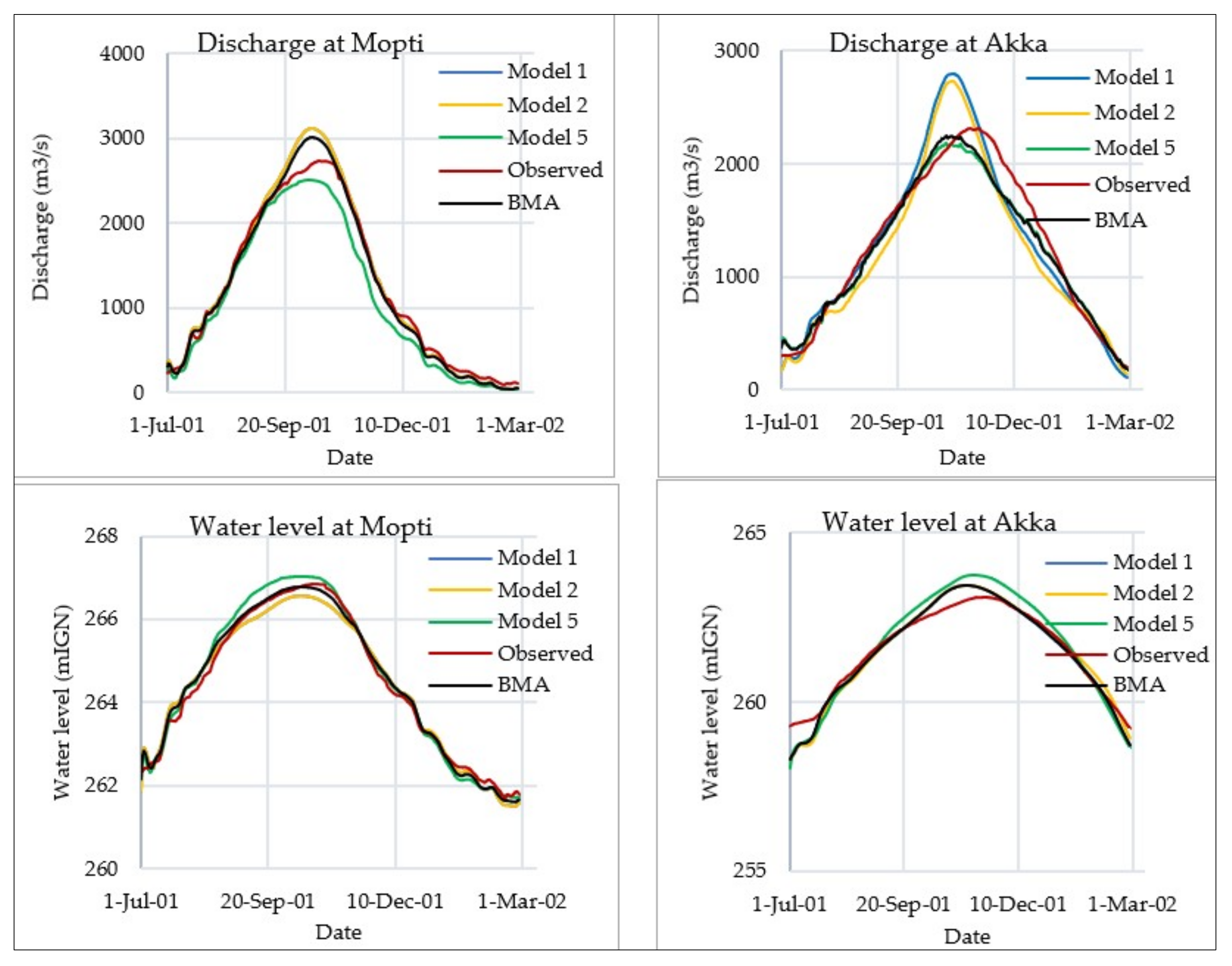
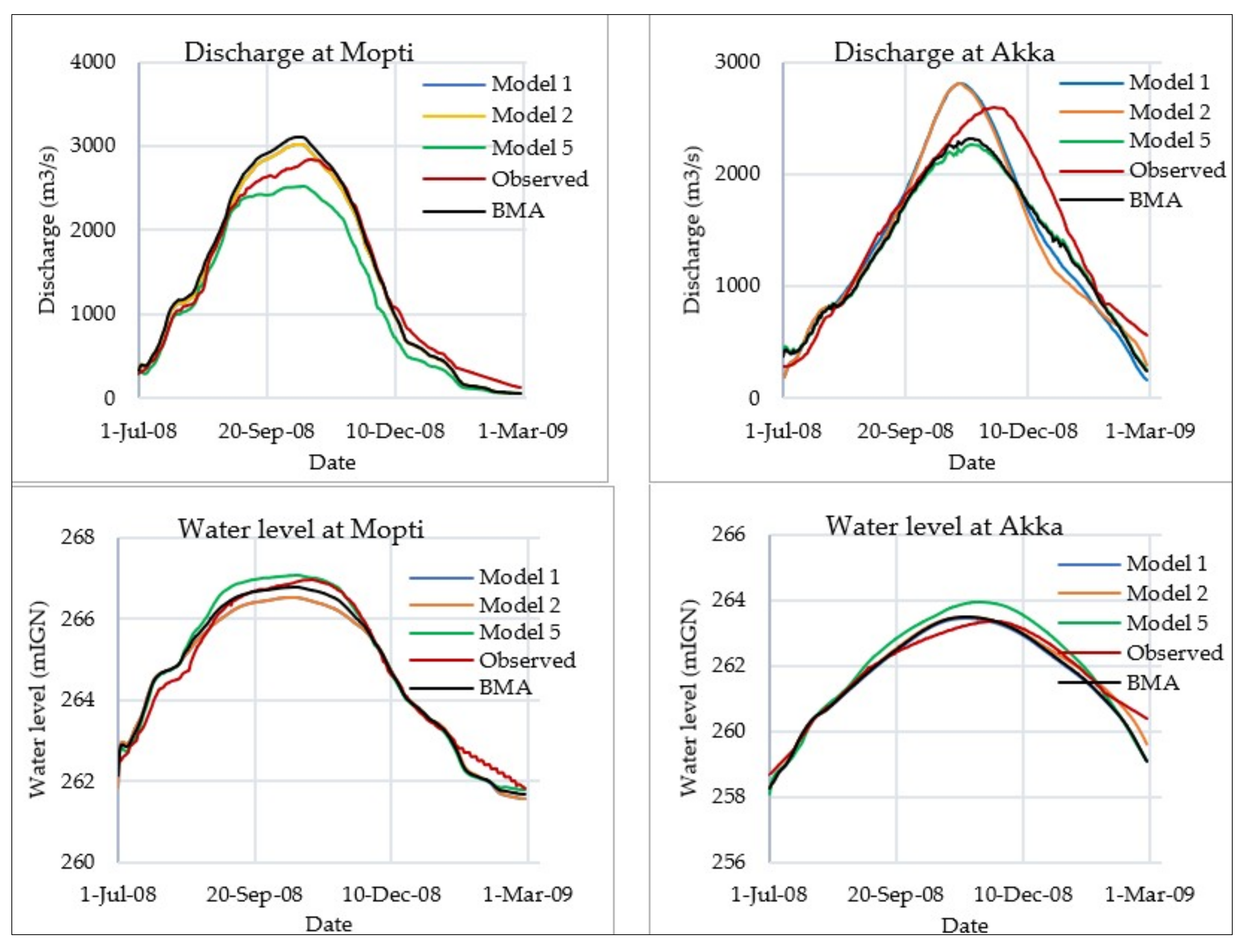
3.1.2. BMA Estimates of Water Levels and Discharge in the Calibration Period

The models were combined based on their respective weight values, as shown in Table 6. The maximum weights of the value of the individual model was found to contribute more to the resultant forecast. For instance, the BMA forecast of discharge at Mopti mainly comes from the combination of Model 2 and Model 3 with 79.31% and 14.17%, respectively, from their simulated discharge. A comparison of the discharge and water level from the best individual models, as well as the BMA prediction at the stations, are given in Figure 8.

The BMA estimate of discharge and water level at the monitoring stations is shown in Figure 8, where there seems to be a good match between observed values (red) and BMA predictions (black). The highest NS values (Figure 9) confirms that BMA outperforms each best individual model.

3.2. Hydrodynamic Models Validation

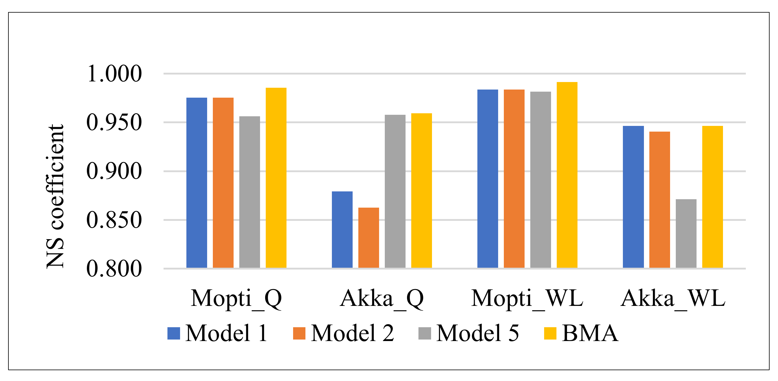
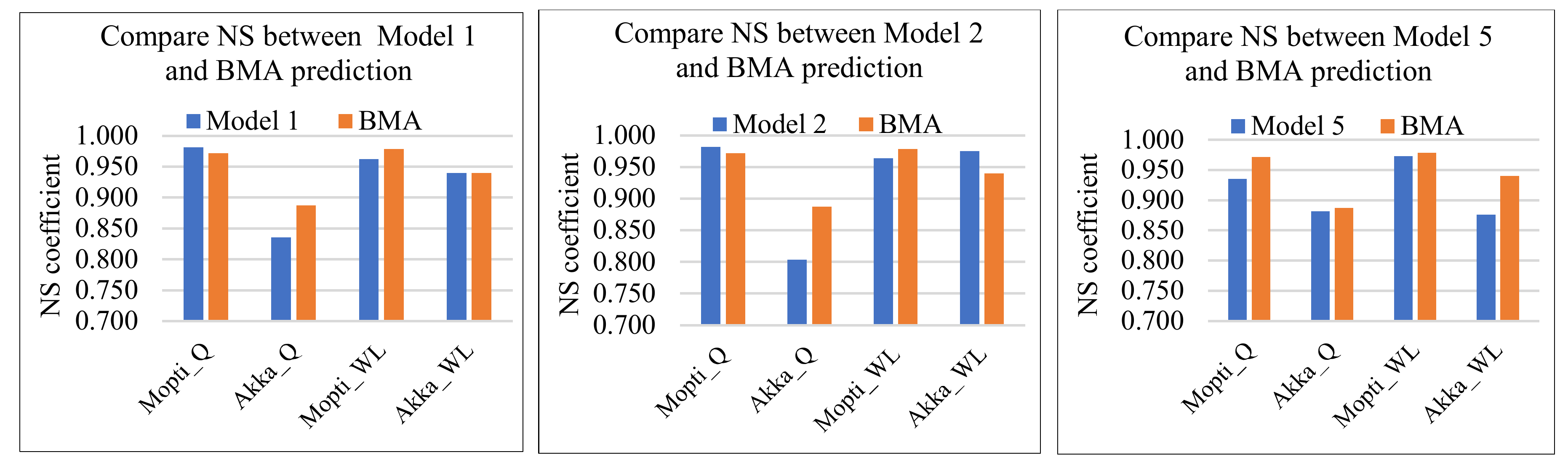
The model results were validated using the 2008–2009 discharge, water levels, and water extent. Each of the models was run with inflows of 2008–2009 at the model inlets keeping the same parameters as obtained at the calibration.

Table 10. Correlation (r) and NS coefficients for simulated discharge and water level in the validation period.

Models	Discharge				Water Level
	Mopti		Akka		Mopti		Akka
	NS	r	NS	R	NS	r	NS	r
Model 1	0.982	0.995	0.836	0.918	0.962	0.984	0.940	0.992
Model 2	0.982	0.995	0.803	0.979	0.964	0.997	0.975	0.994
Model 3	0.939	0.995	0.830	0.979	0.933	0.997	0.917	0.994
Model 4	0.939	0.995	0.800	0.975	0.939	0.997	0.953	0.996
Model 5	0.935	0.990	0.882	0.976	0.973	0.993	0.876	0.988
Model 6	0.935	0.990	0.857	0.975	0.974	0.993	0.881	0.995
BMA	0.972	0.995	0.887	0.972	0.978	0.990	0.940	0.983

summarizes the NS and “r” statistics of the model simulations.

3.3. BMA Validation

The weights obtained from the calibration periods were used to compute BMA predictions for the validation period. The performance statistics, including NS and “r”, were again employed to examine the consistency of the BMA predictions. A comparison of NS statistics between BMA and each of the models 1, 2, and 5 are shown in Figure 10.

Discharge and water levels simulated by Models 1, 2, and 5 have been compared to BMA estimates in Figure 11. The figure shows a good match between observed values (red) and BMA predictions (black).

It can be seen that the BMA predictions perform better than the best individual in most of the cases. Minor degradation of NS statistics also took place; for instance, BMA performance in the validation is slightly worse than that of Models 1 and 2 in predicting discharge at Mopti and the water level at Akka, respectively. Although there is some minor degradation in the performance when the BMA result is compared with the best individual models, BMA is generally superior to that of the individual models, which is consistent with previous studies [52,61]. The improvement due to BMA is relatively low when NS is close to 1, as there is then little room for improvement. When the NS is low, like in the simulation of discharge at Akka (Figure 9 and Figure 10), the improved accuracy is much more obvious. The use of BMA for estimating both variables is, therefore, preferable to the use of individual model simulations. This feature of BMA is particularly interesting in data-scarce environments, such as Mali, where the only available information often comes from global sources with rather coarse resolutions.

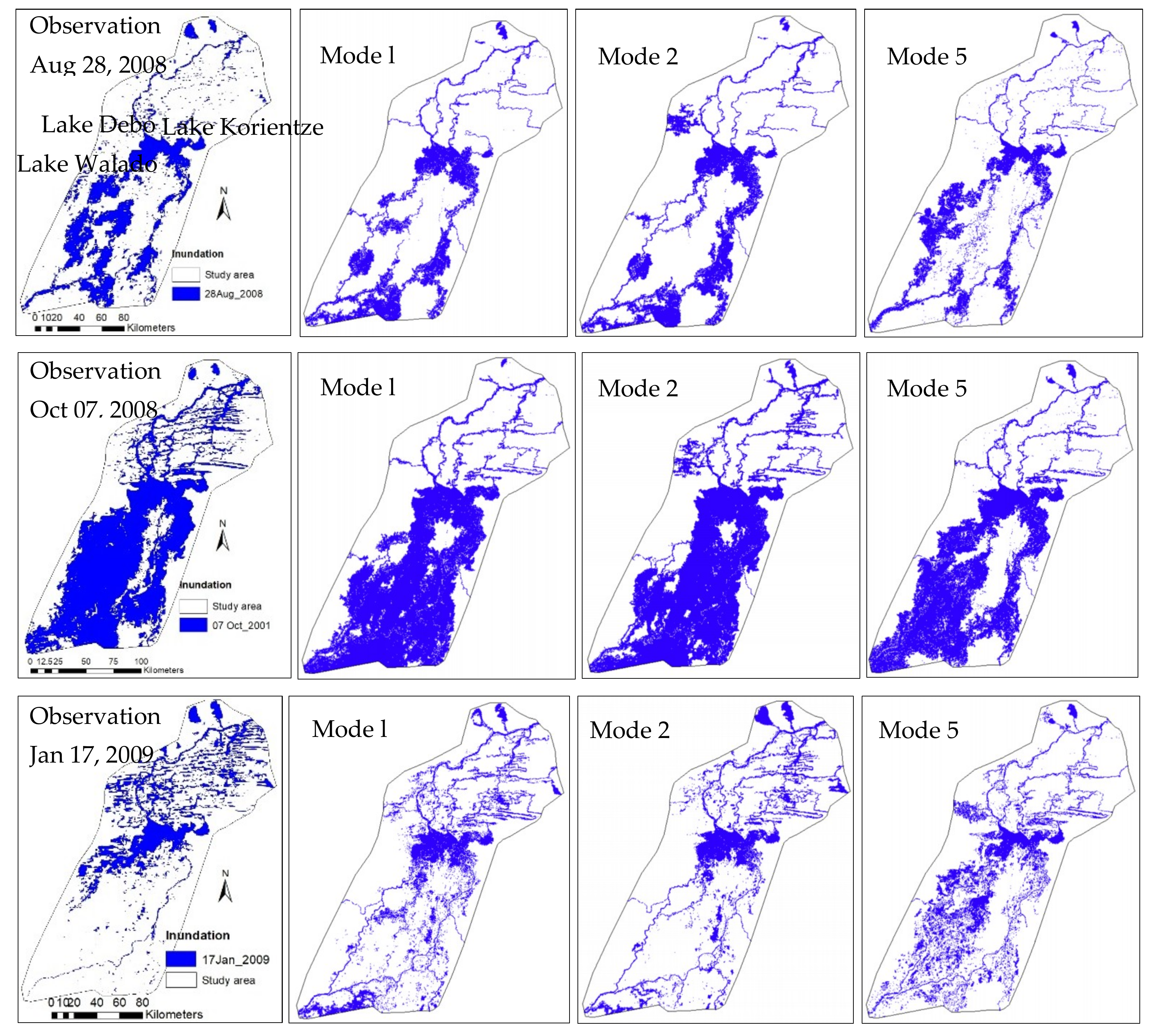
3.4. Simulated Inundation Extent from Best Individual Models

This section provides a brief comparison between simulated and satellite-derived inundation extents for 2008–2009. Only the best individual models (Models 1, 2, and 5), as obtained from Section 3.1.1, are considered in the comparison. The reference inundation extents were derived from MODIS imagery for three days, representing the rising, peak, and recession limb of the 2008–2009 hydrograph. These images were taken on 28 August 2008, 7 October 2008, and 17 January 2009. The inundation extent simulated with Models 1, 2, and 5 along with the satellite-derived inundation extent is shown in Figure 12. The simulated inundation in the central part of the study area, containing Lakes Walado, Debo, and Korientze, shows better agreement with the observed inundation for Model 5 for almost all the three days. The flood extent between KeMacina and Akka on 28 August was better simulated by Model 5 than Models 1 and 2. The inundation pattern simulated by Model 5 also closely matched with the observed inundation on 7 October.

It was also found that, while Model 5 performed well in reproducing the inundation extent of 28 August 2008 and 7 October 2008, it performed poorly in reproducing the inundation extent of 17 January 2009 (receding flood), especially in the area between Ke-Macina and Akka. The simulations show water in interconnecting channels that seem to be dry in the satellite images. This, however, has to be interpreted with care, as the coarse resolution of the MODIS images (500 m) does not allow the detection of narrow channels.

Based on the above facts, we can consider Model 5 to be the best in terms of simulating inundation. It is worth mentioning here that among the individual models, Model 5 was calibrated against inundation obtained from Landsat images captured in the 2001–2002 season. This probably makes this particular model the best among the participating models in simulating inundation extent.

3.5. Potential Usages of the Developed Model

The IND is a complex floodplain that is used by 1.5 million people, where there is little information about floodplain dynamics. Simple empirical equations are used to link water levels at key stations to inundation extents, and flood forecasting is done using linear regressions [62]. A hydrodynamic model, even if not perfect, provides more insight into the flood dynamics, and will be more useful for decision making. The model developed here will be later used to replace or improve the empirical relationships currently used by local authorities, and to develop a process-based flood forecasting model.

4. Conclusions

In this study, six different hydrodynamic models of the Inner Niger Delta (IND) in Mali were developed using three different DEMs and two different downstream boundary conditions. The elevation data came from two global DEMS (SRTM and MERIT), as well as a DEM derived from satellite imagery and water level observations using waterline methods. Given the data scarcity in the area, a considerable amount of input data, such as bathymetry, the river network, friction coefficient, and inundation extent were derived from secondary sources, leading to a high level of uncertainty in the simulations. The six models which were developed showed unequal performances in simulating water levels, discharges, and floodplain extent, with none of them outperforming the others in all fronts. It was found that specifying the boundary condition (water levels as a function of discharge) led to better results. The reason for this seems to the use of the relaxation coefficient in the algorithm of the stage-discharge curve. Overall, the MERIT DEM was the best DEM among the ones considered in this paper, as it is a processed DEM by removing errors from SRTM. Bayesian Model Averaging (BMA) was used to produce a more robust estimate of water levels and discharges. BMA also helped to identify which individual models had the highest value for an end-user who is more interested in a particular location in the IND and a particular hydraulic variable.

References

1. Zwarts, L.; Frerotte, J. Water Crisis in the Inner Niger Delta (Mali), Causes, Consequences, Solutions; A&W-Report 1832; Altenburg & Wymenga Ecologisch Onderzoek: Feanwâlden, The Netherlands, 2012. [Google Scholar]
2. Zwarts, L.; Van Beukering, P.; Kone, B.; Wymenga, E. The Niger, a Lifeline. Effective Water Management in the Upper Niger Basin. RIZA, Lelystad/Wetlands International, Sévaré; Institute for Environmental studies (IVM): Amsterdam, The Netherlands; A&W Ecological Consultants: Veenwouden, Mali, The Netherlands, 2005. [Google Scholar]
3. Liersch, S.; Fournet, S.; Koch, H. Assessment of Water Management and Climate Change Impacts on the Water Resources in the Upper Niger and Bani River Basins; BAMGIRE Programme Final Report; Potsdam Institute for Climate Impact Research: Potsdam, Germany; Wetlands International: Mali, The Netherlands, 2019. [Google Scholar]
4. CDKN. The IPCC’s Fifth Assessment Report: What’s in It for Africa? Overseas Development Institute/Climate and Development Knowledge Network: London, UK, 2014; 35p, Available online: https://cdkn.org/wp-content/uploads/2014/04/AR5_IPCC_Whats_in_it_for_Africa.pdf (accessed on 14 January 2019).
5. USAID. Climate Risk in Mali: Country Risk Profile. Available online: https://www.climatelinks.org/sites/default/files/asset/document/Mali_CRP_Final.pdf (accessed on 12 January 2019).
6. Liersch, S.; Fournet, S.; Koch, H.; Djibo, A.G.; Reinhardt, J.; Kortlandt, J.; Van Weert, F.; Seidou, O.; Klop, E.; Baker, C.; et al. Water resources planning in the Upper Niger River basin: Are there gaps between water demand and supply? J. Hydrol. Reg. Stud. 2019, 21, 176–194. [Google Scholar] [CrossRef]
7. Neal, J.; Schumann, G.; Bates, P. A subgrid channel model for simulating river hydraulics and floodplain inundation over large and data sparse areas. Water Resour. Res. 2012, 48, W11506. [Google Scholar] [CrossRef]
8. Bates, P.D.; de Roo, A. A simple raster-based model for flood inundation simulation. J. Hydrol. 2000, 236, 54–77. [Google Scholar] [CrossRef]
9. Dadson, S.J.; Ashpole, I.; Harris, P.; Davies, H.N.; Clark, D.B.; Blyth, E.; Taylor, C.M. Wetland inundation dynamics in a model of land surface climate: Evaluation in the Niger inland delta region. J. Geophys. Res. 2010, 115, D23114. [Google Scholar] [CrossRef]
10. Haag, A.V. Coupling A Large-Scale Hydrological Model to a High-Resolution Hydrodynamical Model, A Study of Floods within the Niger Inner Delta as a First Step towards a Potential Global Application. Master’s Thesis, Department of Physical Geography and Faculty of Geoscience, Utrecht University, Utrecht, The Netherlands, 2015. [Google Scholar]
11. Kernkamp, H.W.J.; van Dam, A.; Stelling, G.S.; de Goede, E.D. Efficient scheme for the shallow water equations on un-structured grids with application to the Continental Shelf. Ocean Dynam. 2011, 61, 1175–1188. [Google Scholar] [CrossRef]
12. Deltares. D-Flow Flexible Mesh, User Manual, draft version; Deltares: Delft, The Netherlands, 2015. [Google Scholar]
13. Hervouet, J.M. Hydrodynamics of Free Surface Flows Modelling with the Finite Element Method; Wiley: New York, NY, USA, 2007. [Google Scholar]
14. NASA JPL. NASA Shuttle Radar Topography Mission Global 1 arc second, NASA EOSDIS Land Processes DAAC. 2013. Available online: https://earthexplorer.usgs.gov/ (accessed on 1 September 2016).
15. Yamazaki, D.; Ikeshima, D.; Tawatari, R.; Yamaguchi, T.; O’Loughlin, F.; Neal, J.C.; Sampson, C.C.; Kanae, S.; Bates, P.D. A high accuracy map of global terrain elevations. Geophys. Res. Lett. 2017, 44, 5844–5853. [Google Scholar] [CrossRef]
16. Rodríguez, E.; Morris, C.S.; Belz, J.E. A global assessment of the SRTM performance. Photogramm. Eng. Remote Sens. 2006, 72, 249–260. [Google Scholar] [CrossRef]
17. Cracknell, A.P.; Hayes, L.W.B.; Keltie, G.F. Remote sensing of the Tay Estuary using visible and near infra-red data: mapping of the inter-tidal zone. Proc. R. Soc. Edinb. 1987, 92B, 223–236. [Google Scholar]
18. Ramsey, E.W. Monitoring Flooding in coastal wetlands by using radar imagery and ground-based measurements. Int. J. Remote Sens. 1995, 16, 2495–2502. [Google Scholar] [CrossRef]
19. Mason, D.C.; Davenport, I.J.; Flather, R.A.; Gurney, C. A digital elevation model of the inter-tidal areas of the Wash, England, produced by the waterline method. Int. J. Remote Sens. 1998, 9, 1455–1460. [Google Scholar] [CrossRef]
20. Arnold, J.G.; Srinivasan, R.; Muttiah, R.S.; Williams, J.R. Large area hydrologic modeling and assessment—Part 1: Model development. J. Am. Water Resour. Assoc. 1998, 34, 73–89. [Google Scholar] [CrossRef]
21. Hoeting, J.A.; Madigan, D.; Raftery, A.E.; Volinsky, C.T. Bayesian model averaging: A tutorial. Stat. Sci. 1999, 14, 382–417. [Google Scholar]
22. Schumann, G.J.-P.; Andreadis, K.M.; Bates, P.D. Downscaling coarse grid hydrodynamic model simulations over large domains. J. Hydrol. 2014, 508, 289–298. [Google Scholar] [CrossRef]
23. Biancamaria, S.; Bates, P.; Boone, A.; Mognard, N. Large-scale coupled hydrologic and hydraulic modelling of the Ob river in Siberia. J. Hydrol. Elsevier 2009, 379, 136–150. [Google Scholar] [CrossRef] [Green Version]
24. JAXA. ALOS World 3D-30m (AW3D30), Version 2, Global Digital Surface Model, Earth Observation Research Center (EORC), Japan Aerospace Exploration Agency. 2018. Available online: https://www.eorc.jaxa.jp/ALOS/en/aw3d30/index.htm (accessed on 10 September 2017).
25. Hawker, L.; Bates, P.; Neal, J.; Rougier, J. Perspectives on Digital Elevation Model (DEM) Simulation for Flood Modeling in the Absence of a High-Accuracy Open Access Global DEM. Front. Earth Sci. 2018, 6, 233. [Google Scholar] [CrossRef]
26. Archer, L.; Neal, J.C.; Bates, P.C.; House, J.I. Comparing TanDEM-X data with frequently-used DEMs for Flood inundation modelling. Water Resour. Res. 2018. [Google Scholar] [CrossRef]
27. Xu, H. Modification of normalized difference water index (NDWI) to enhance open water features in remotely sensed imagery. Int. J. Remote Sens. 2006, 27, 3025–3033. [Google Scholar] [CrossRef]
28. Wilson, E.H.; Sader, S.A. Detection of forest harvest type using multiple dates of Landsat TM imagery. Remote Sens. Environ. 2002, 80, 385–396. [Google Scholar] [CrossRef]
29. Ogilvie, A.; Belaud, G.; Delenne, C.; Bailly, J.; Bader, J.; Oleksiak, A.; Ferry, L.; Martin, D. Decadal monitoring of the Niger Inner Delta flood dynamics using MODIS optical data. J. Hydrol. Elsevier 2015, 523, 368–383. [Google Scholar] [CrossRef] [Green Version]
30. Leopold, L.B.; Maddock, T.J. The hydraulic geometry of stream channels and some physiographic implications. U.S. Geol. Surv. Prof. Pap. 1953, 252, 1–57. [Google Scholar]
31. Hey, R.D.; Thorne, C.R. Stable channels with mobile gravel beds. J. Hydraul. Eng. 1986, 112, 671–689. [Google Scholar] [CrossRef]
32. Leopold, L.B. A View of the River: Cambridge, Mass; Harvard University Press: Cambridge, MA, USA, 1994. [Google Scholar]
33. Seidou, O. Development of Models and Tools in Support of the BAMGIRE Program; Final Report; Wetlands International and University of Ottawa: Ottawa, ON, Canada, 2019. [Google Scholar]
34. Arnold, J.G.; Moriasi, D.N.; Gassman, P.W.; Abbaspour, K.C.; White, M.J.; Srinivasan, R.; Jha, M.K. SWAT: Model use calibration, and validation. Trans. Asabe 2012, 55, 1491–1508. [Google Scholar] [CrossRef]
35. Neitsch, S.L.; Arnold, J.G.; Kiniry, J.R.; Williams, J.R. Soil and Water Assessment Tool, Theoretical Documentation: Version 2005; USDA Agricultural Research Service and Texas A&M Blackl and Research Center: Temple, TX, USA, 2005.
36. USDA Soil Conservation Service. National Engineering Handbook; Section 4, Hydrology; US Government Printing Office: Washington, DC, USA, 1972.
37. Monteith, J.L. Evaporation and environment. In The State and Movement of Water in Living Organisms; Fogg, G.F., Ed.; Cambridge University Press: Cambridge, UK, 1965; pp. 205–234. [Google Scholar]
38. Abbaspour, K.C. User Manual for SWAT-CUP, SWAT Calibration and Uncertainty Analysis Programs; Swiss Federal Institute of Aquatic Science and Technology, Eawag: Dübendorf, Switzerland, 2007; Available online: https://www.eawag.ch/de/abteilung/siam/software/ (accessed on 16 June 2017).
39. Maiga, F. Hydrological Impacts of Irrigation Schemes and Dams Operation in the Upper Niger Basin and Inner Niger Delta. Master’s Thesis, University of Ottawa, Ottawa, ON, Canada, 2019. [Google Scholar]
40. Loveland, T.R.; Reed, B.C.; Brown, J.F.; Ohlen, D.O.; Zhu, Z.; Yang, L.; Merchant, J.W. Development of a global land cover characteristics database and IGBP DISCover from 1 km AVHRR data. Int. J. Remote Sens. 2000, 21, 1303–1330. [Google Scholar] [CrossRef]
41. Asante, K.O.; Artan, G.A.; Pervez, S.; Bandaragoda, C.; Verdin, J.P. Technical Manual for the Geospatial Stream Flow Model (GeoSFM): U.S. Geological Survey Open-File Report; U.S. Geological Survey: Reston, VI, USA, 2008; 65p. Available online: https://pubs.usgs.gov/of/2007/1441/pdf/ofr2008-1441.pdf (accessed on 21 September 2018).
42. Marchuk, G.I. Methods of Numerical Mathematics; Springer: New York, NY, USA, 1975; 316p. [Google Scholar]
43. Brookes, A.N.; Hughes, T.J.R. Streamline Upwind/Petrov-Galerkin formulations for convection dominated flows with particular emphasis on the incompressible Navier-Stokes Equations. Comput. Methods Appl. Mech. Eng. 1982, 32, 199–259. [Google Scholar] [CrossRef]
44. Bates, P.D.; Anderson, M.G.; Hervouet, J.-M.; Hawkes, J.C. Investigating the behavior of two-dimensional finite element models of compound channel flow. Earth Surf. Process. Landf. 1997, 22, 3–17. [Google Scholar] [CrossRef]
45. Zwarts, L. Will the Inner Niger Delta Shrivel up due to Climate Change and Water Use Upstream? A&W Rapport 1537; Altenburg & Wymenga Ecologisch Onderzoek: Feanwâlden, The Netherlands, 2010. [Google Scholar]
46. Woodhead, S.; Asselman, N.; Zech, Y.; Soares-Frazao, S.; Bates, P.; Kortenhaus, A. Evaluation of Inundation Models; FLOODsite Report T08-07-01. 2007. Available online: https://ecapra.og/sites/default/files/documents/Flood%20Inundation%20Modelling.pdf (accessed on 6 August 2019).
47. Aronica, G.; Hankin, B.; Beven, K. Uncertainty and equifinality in calibrating distributed roughness coefficients in a flood propagation model with limited data. Adv. Water Resour. 1998, 22, 349–365. [Google Scholar] [CrossRef]
48. Pappenberger, F.; Beven, K.; Horritt, M.; Blazkova, S. Uncertainty in the calibration of effective roughness parameters in HEC-RAS using inundation and downstream level observations. J. Hydrol. 2005, 302, 46–69. [Google Scholar] [CrossRef]
49. Schöniger, A.; Wöhling, T.; Nowak, W. Model selection on solid ground: Rigorous comparison of nine ways to evaluate Bayesian model evidence. Water Resour. Res. 2014, 50, 9484–9513. [Google Scholar] [CrossRef]
50. Madigan, D.; Raftery, A.E.; Volinsky, C.; Hoeting, J. Bayesian model averaging. In Proceedings of the AAAI Workshop on Integrating Multiple Learned Models, Portland, OR, USA, 4–5 August 1996; pp. 77–83. [Google Scholar]
51. Raftery, A.E.; Gneiting, T.; Balabdaoui, F.; Polakowski, M. Using Bayesian model averaging to calibrate forecast ensembles. Mon. Weather Rev. 2005, 133, 1155–1174. [Google Scholar] [CrossRef]
52. Duan, Q.; Ajami, N.K.; Gao, X.; Sorooshian, S. Multi-model ensemble hydrologic prediction using Bayesian model averaging. Adv. Water Res. 2007, 30, 1371–1386. [Google Scholar] [CrossRef] [Green Version]
53. Zhu, R.; Zheng, H.; Wang, E.; Zhao, W. Multi-Model Ensemble Simulation of Flood Events using Bayesian Model Averaging. In Proceedings of the 20th International Congress on Modelling and Simulation, Adelaide, Australia, 1–6 December 2013. [Google Scholar]
54. Beckers, J.V.L.; Sprokkereef, E.; Roscoe, K.L. Use of Bayesian Model Averaging to Determine Uncertainties in River Discharge and Water Level Forecasts. In Proceedings of the 4th International Symposium on Flood Defence: Managing Flood Risk, Reliability and Vulnerability, Toronto, ON, Canada, 6–8 May 2008. [Google Scholar]
55. Raftery, A.E. Bayesian Model Selection in Structural Equation Models. In Testing Structural Equation Models; Bollen, K.A., Long, J.S., Eds.; Sage: Beverly Hills, CA, USA, 1993; pp. 163–180. [Google Scholar]
56. Draper, D. Assessment and propagation of model uncertainty. J. R. Stat. Soc. Ser. B 1995, 57, 45–97. [Google Scholar] [CrossRef]
57. Vrugt, J.A.; Diks, C.G.; Clark, M.P. Ensemble bayesian model averaging using markov chain monte carlo sampling. Environ. Fluid Mech. 2008, 8, 579–595. [Google Scholar] [CrossRef]
58. McLachlan, G.J.; Krishnan, T. The EM Algorithm and Extensions; Wiley: New York, NY, USA, 1997. [Google Scholar]
59. Pappenberger, F.; Matgen, P.; Beven, K.J.; Henry, J.B.; Pfister, L.; Fraipont, P. Influence of uncertain boundary conditions and model structure on flood inundation predictions. Adv. Water 2006, 29, 1430–1449. [Google Scholar] [CrossRef]
60. Guthke, A.; Höge, M.; Nowak, W. Bayesian model evidence as a model evaluation metric, Geophysical Research Abstracts, Volume 19, EGU2017-PREVIEW, EGU General Assembly. 2017. Available online: https://meetingorganizer.copernicus.org/EGU2017/EGU2017-13390-1.pdf (accessed on 8 August 2019 ).
61. Vrugt, J.A.; Robinson, B.A. Treatment of uncertainty using ensemble methods: Comparison of sequential data assimilation and Bayesian Model Averaging. Water Resour. Res. 2007, 43, W01411. [Google Scholar] [CrossRef]
62. OPIDIN. Forecast Tool to Predict the Inundations in the Inner Niger Delta. Available online: https://www.opidin.org/en/home (accessed on 9 August 2019).
Figure 1. Location map of the study area, the Inner Niger Delta, Mali, West Africa.
Water 11 01766 g001
Figure 2. Hydrodynamic model domain, along with dams and reservoirs in the Upper Niger basin.
Water 11 01766 g002
Figure 3. Digital elevation model derived from the waterline method (left), Shuttle Radar Topography Mission (SRTM) (middle), and Multi-Error-Removed Improved-Terrain (MERIT DEM) (right).
Water 11 01766 g003
Figure 4. Satellite Images of inundation extents of the Delta on 28 July 2001 (left) and 16 October 2001 (right) (Source: Zwarts, et al., 2005).
Water 11 01766 g004
Figure 5. River network for the model.
Water 11 01766 g005
Figure 6. (a) Extent of the SWAT model with calibration stations (Source: Seidou, 2019) and (b) locations of the liquid boundaries in the hydrodynamic model.
Water 11 01766 g006
Figure 7. Manning’s coefficient at the floodplain of Inner Niger Delta (IND).
Water 11 01766 g007
Figure 8. Comparison of discharge (top) and water level (bottom) of the best models and BMA.
Water 11 01766 g008
Figure 9. Comparison of the Nash-Sutcliffe (NS) coefficient of BMA and the three best individual models.
Water 11 01766 g009
Figure 10. Comparison of NS coefficient of BMA to each of Models 1,2, and 5.
Water 11 01766 g010
Figure 11. Comparison of discharge (top) and water level (bottom) from the best individual models and BMA prediction at the validation.
Water 11 01766 g011
Figure 12. Inundation extent on 28 August 2008 (left panel), 7 October 2008 (middle), and 17 January 2009 (right panel).
Water 11 01766 g012