Article

The Spatiotemporal Variability of Evapotranspiration and Its Response to Climate Change and Land Use/Land Cover Change in the Three Gorges Reservoir

1
State Key Laboratory of Simulation and Regulation of Water Cycle in River Basin, China Institute of Water Resources and Hydropower Research, Beijing 100038, China
2
Department of Hydraulic Engineering, Tsinghua University, Beijing 100084, China
3
School of Water Conservancy Engineering, North China University of Water Resources and Electric Power, Zhengzhou 450011, China
*
Author to whom correspondence should be addressed.
Water 2019, 11(9), 1739; https://doi.org/10.3390/w11091739
Submission received: 15 July 2019 / Revised: 8 August 2019 / Accepted: 19 August 2019 / Published: 21 August 2019
(This article belongs to the Special Issue Effects of Climate Change on Water Resources)

Abstract

:
Evapotranspiration (ET) has undergone profound changes as a result of global climate change and anthropogenic activities. The construction of the Three Gorges Reservoir (TGR) has led to changes in its land use/land cover (LUCC) and local climate, which in turn has changed ET processes in the TGR region. In this paper, the CLM4.5 land surface model is used to simulate and analyze the spatiotemporal variability of ET between 1993 and 2013. Four experiments were conducted to quantify the contribution rate of climate change and LUCC to changes in ET processes. The results show that the climate showed a warming and drying trend from 1993 to 2013, and the LUCC indicates decreasing cropland with increasing forest, grassland, water bodies and urban areas. These changes increased the mean annual ET by 13.76 mm after impoundment. Spatially, the vegetation transpiration accounts for the largest proportion in ET. The decreasing relative humidity and increasing wind speeds led to an increase in vegetation transpiration and ground evaporation, respectively, in the center of the TGR region, while the LUCC drove changes in ET in water bodies, urban areas and high-altitude regions in the TGR region.

1. Introduction

Evapotranspiration (ET) is one of the vital links in the water and energy balance between the land surface and atmosphere. ET occurs through the mutual transfer of water and energy between soil, vegetation and the atmosphere [1] and interacts with the climate system. Climate change affects the water cycle process and can lead to changes in ET [2], while changes in ET can also adversely affect the climate across local and regional scales [3,4]. In recent years, the terrestrial ecosystem has undergone vast changes as a result of the increasing impact of anthropogenic activities which have led to the intensification of global climate change. The urbanization and the construction of large scale hydraulic engineering projects has led to a reduction of vegetation coverage and the excessive felling of trees. The exploitation of forest resources has led to a sharp decline in forest areas and the overuse of water resources has caused persistent drought and desertification in some areas. These and other anthropogenic activities have resulted in a series of climatic and ecological environmental issues [5], which have caused the attention of governments and scientific researchers. As a critical element of ecosystems and the global climate system, the study on ET and its response to climate change and land use/land cover (LUCC) is critical to understand how climate change and human activities influence the energy balance processes and the water cycle in terrestrial ecosystems.
The Three Gorges Project was started in 1994 and began impoundment in June 2003. The water table of the reservoir reached 135 m in June 2003, 156 m in October 2006, and 175 m in October 2010 [6]. The Three Gorges Project has brought economic and social benefits to the region such as flood control, power generation and shipping, and the Three Gorges Reservoir (TGR) is a unique region formed after the Three Gorges Project was carried out in China. With the construction and operation of the TGR, a series of far-reaching changes have taken place in the land use/land cover of the region. In addition, the main projects such as resettlement, urban relocation and the development of supporting facilities, have caused further pressure on the local ecosystem and climate system [7]. According to Reder et al., the temperature in the TGR will increase by at least 1 °C under the RCP 4.5 and 8.5 scenarios. However, the changes in precipitation are more complicated, with a decrease in the dry season and an increase in the rainy season [8]. The water cycle process in the TGR is also likely to change greatly. Therefore, taking the TGR as an example, can not only improve our understanding of ET in the water cycle and energy balance processes in the region, but also provide decision supports for water resource allocation and management, and it is of great significance for maintaining the ecological security and the sustainable development of the social economy under the changing environment.
In recent years, extensive efforts have been carried out to understand the spatiotemporal variability of ET under a changing climate. This work mainly used statistical methods to detect the abrupt point of climate change, and then analyze the variation trend of ET before and after the abrupt point [9]. One type of research focuses on reference ET [10], calculated using the Penman-Monteith equation [11,12], and another focuses on the actual ET. Since actual ET data is difficult to obtain through observation, a water balance model [13,14] or remote sensing model [15] are usually used to indirectly obtain the actual ET. The effect of LUCC on ET is typically assessed using a land surface model and inputting different land use types into the model for sensitivity experiments [16,17,18,19]. At present, a small amount of work has been done to simultaneously consider the impact of climate change and LUCC on ET [20,21]. A more common approach is to combine meteorological data with remote sensing data to analyze the relationship between various meteorological factors, land use types and ET [22], and to separate the contribution rate of climate change and LUCC to changes in ET [23,24]. However, these statistical methods lack understanding of intrinsic mechanisms associated with ET and are, therefore, difficult to apply in new situations. Therefore, this study aims to perform multiple sets of numerical simulation experiments using the CLM4.5 land surface model to: (1) Analyze the variability of climatic factors and land use/land cover; (2) characterize the spatial and temporal variability of ET in the TGR region from 1993 to 2013; (3) quantify individual contributions of climate change and LUCC to the variability of ET.

2. Materials and Methods
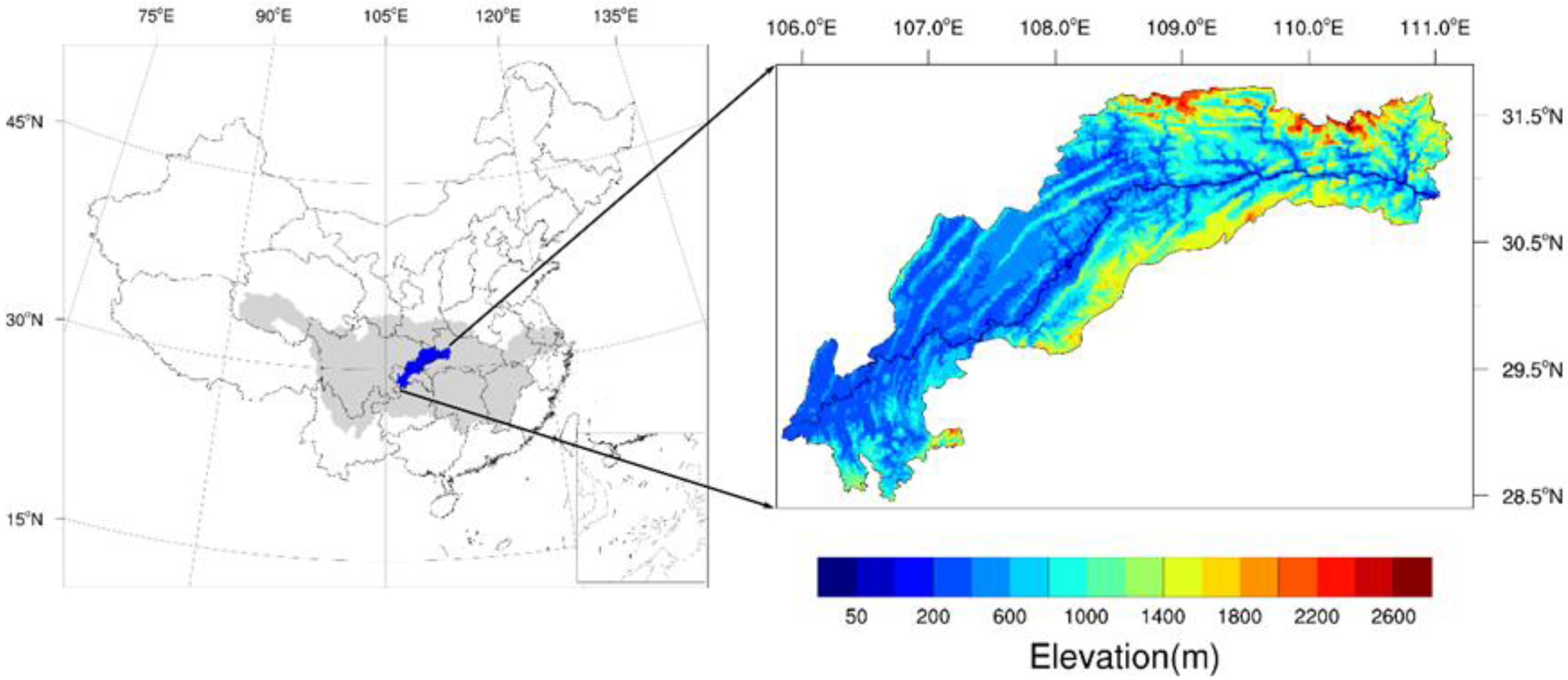
2.1. Study Area

The TGR region refers to the catchment area between the dam site and the end of the backwater of the reservoir after the successful impoundment of the TGR. Located at the end of the upper reaches of the Yangtze River Basin (28.46°–31.73° N, 105.84°–111.13° E), the TGR region is shaped like a narrow strip. It covers a total area of 59,326 km2 with a main channel length of 658 km. As the TGR region is situated at the intersection of three tectonic units, the Daba fold belt, the Eastern Sichuan fold belt, and the Sichuan-Hubei-Hunan-Guizhou uplifted belt, the terrain is undulating, and the height difference is approximately 1000–1500 m. The climate, which is affected by the canyon topography, is characterized by warm winters, early springs, hot summers, and late autumns, and generally has high humidity and often clouds and fogs. The annual average temperature is 15–18 °C and the vertical change in temperature is rapid. The rainfall is abundant in the region all year round although the summer rainfall accounts for 40% of the average annual precipitation of approximately 1150.26 mm. The land use types in the region are mainly farmland, woodland, and grassland. With a continuous rise in the flooding line in the region and the subsequent resettlement, migration, and reconstruction of towns and supporting facilities, the land use/land cover in the region has undergone frequent changes. The TGR region is shown in Figure 1.

2.2. Data

The data used in this study include atmospheric forcing data and surface data required to run the land surface model and remote sensing data to validate the simulation results. The China Meteorological Forcing Dataset [25], with a temporal resolution of 3 h and a horizontal spatial resolution of 0.1 degree, was used to drive the land surface model. The dataset was produced by merging a variety of data sources including China Meteorological Administration station data, TRMM satellite precipitation analysis data, GLDAS data, GEWEX-SRB radiation data, and Princeton forcing data [26]. The dataset includes seven elements, near surface air temperature, near surface air pressure, near surface air specific humidity, near surface wind speed, surface downward shortwave radiation, surface downward longwave radiation, and a precipitation rate. A 30 m × 30 m ASTER GDEM was used for watershed delineation and stream network formation. The plant function types (PFTs) data reflects the land use/land cover of the study area. Since the land use/land cover changed dramatically before and after the impoundment of the TGR region, the PFTs of 2000 and 2010 were selected to represent the land use/land cover before and after impoundment of the region. A one km China land cover classification map [27] was used for 2000, while the MODIS Land Cover Product MCD12Q1 [28,29] was selected with a spatial resolution of 500 m for 2010. Since the PFTs classification of the MCD12Q1 and the community land model (CLM) is different, the PFTs and climatic factor rules [30] were used for the conversion. The soil database of China for land surface modeling [31] with a spatial resolution of 30 × 30 arc-seconds was used to create the physical and chemical soil parameters for the land surface model. The remote sensing data of the MOD16 monthly ET [32,33] with a spatial resolution of 1 km was used to validate the simulation results. For the convenience of model simulation and validation, all data were converted to 0.01 degree.

2.3. Methods

2.3.1. Description of CLM4.5

The community land model (CLM) 4.5 was developed by the National Center for Atmospheric Research [34], and it is the land component of the community earth system model (CESM) 1.2.0 [35]. The CLM4.5 is a process-based model that simulates biogeophysical and biogeochemical processes. The biogeophysical processes include radiation, momentum, sensible heat and latent heat flux exchange between the land surface and atmosphere, heat transfer in soil and snow, and water cycle processes including precipitation, interception, infiltration, evapotranspiration, and runoff [36]. Biogeochemical processes include vegetation photosynthesis, vegetation phenology, and carbon and nitrogen cycles [37]. A nested subgrid hierarchy is used to represent the spatial surface heterogeneity in the model. Each grid is composed of multiple landunits, columns and PFTs. A landunit is the first subgrid level to capture the widest spatial patterns of subgrid heterogeneity. The second subgrid level is a column, which is used to characterize the potential variability in the soil and snow state variables within a landunit. The third subgrid level involve PFTs, which mainly represent the differences in the biophysical and biogeochemical parameters between broad categories of plants. The model is simulated independently at each subgrid level, and each subgrid level has its own diagnostic variables. For the process of ET, it is partitioned into transpiration, managed by stoma physiology and photosynthesis, and evaporation, which can be further divided into ground evaporation and canopy evaporation according to land use/land cover [38,39].
The four indexes, namely the coefficient of determination (R2), the root mean squared error (RMSE), the absolute error (BIAS) and the Nash-Sutcliffe efficiency coefficient (NSE) were adopted to assess the performance of the CLM4.5 model [40,41]. The R2 represents the goodness of fit between the simulated and observed ET. The RMSE reflects the degree of dispersion. The BIAS measures the degree of deviation, and the NSE describes the predictive power of the model. The formulas are shown as follows:
y i = a S i + b
R 2 = i = 1 N ( y i O ¯ ) 2 i = 1 N ( O i O ¯ ) 2
R M S E = i = 1 N ( S i O i ) 2 n
B I A S = i = 1 N ( S i O i )
N S E = 1.0 i = 1 N ( O i S i ) 2 i = 1 N ( O i O ¯ ) 2
where, a is the slope of linear regression line, b is the intercept of linear regression line, Oi is the observed ET, Si is the simulated ET, O ¯ is the average observed ET, and N is the number of time series.

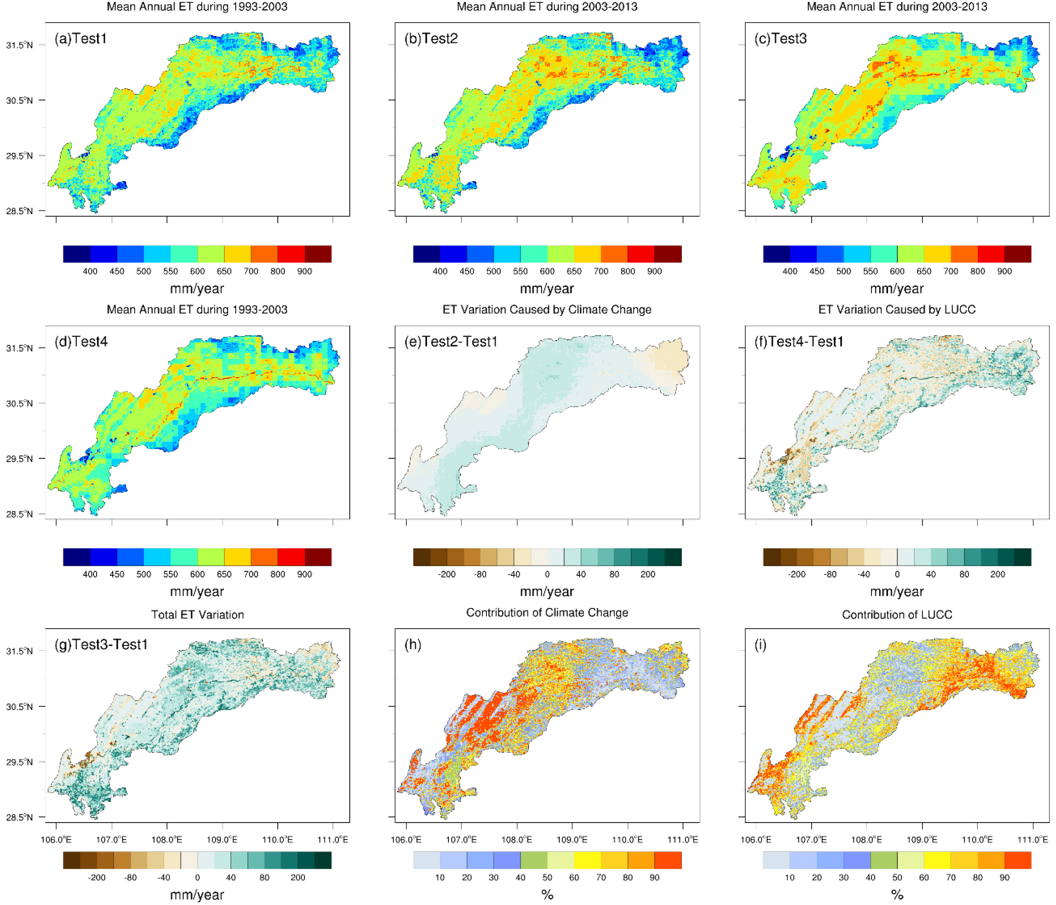
2.3.2. Experimental Design

In order to study the spatiotemporal variability of ET before and after the impoundment, 10 years before and after the beginning of impoundment in June 2003, that is June 1993 to May 2013, was taken as the research period. The spatial resolution was set to 0.01 degree and the output frequency was 24 h to obtain the finer resolution simulated results. It was assumed that climate change and LUCC were the two factors that caused the variation of ET. The formula could be expressed as follows:
Δ E T t o t a l = Δ E T c l i m a t e + Δ E T L U C C
C c l i m a t e = Δ E T c l i m a t e Δ E T t o t a l
C L U C C = Δ E T L U C C Δ E T t o t a l
where, Δ E T t o t a l is the total variation in ET, Δ E T c l i m a t e is the variation caused by climate change, Δ E T L U C C is the variation caused by LUCC, C c l i m a t e is the contribution rate of climate change and C L U C C is the contribution rate of LUCC.
As shown in Table 1, four simulation tests using CLM4.5 were conducted to explore the response of ET to climate change and LUCC. Test 1 simulated the actual situation from June 1993 to May 2003. Test 2 simulated ET from June 2003 to May 2013 under the land use/land cover condition in 2000. Test 3 simulated the actual situation from June 2003 to May 2013. Test 4 simulated the ET from June 1993 to May 2003 under the land use/land cover condition in 2010. According to Formulas (6)–(8), the difference between Test 2 and Test 1 is the variability in ET caused by climate change. The difference between Test 4 and Test 1 represents the variability in ET caused by LUCC, while the difference between Test 3 and Test 1 gives the total variability in ET.
Before the four tests, two spin-ups of 50 years were performed using the CLM4.5 model to provide a balanced climatology. They were driven by the atmospheric forcing data from June 1983 to May 1993 for five times under the land use/land cover condition in 2000 and 2010, respectively. For the four tests, Test 1 used the final state in May 1993 under the land use/land cover condition in 2000 as the initial condition, and Test 2 used the final state of Test 1 as the initial condition. Similarly, Test 4 used the final state in May 1993 under the land use/land cover condition in 2010 as the initial condition and Test 3 used the final state of Test 4 as the initial condition.

2.3.3. Trend Analysis

A linear regression equation was adopted to assess the trend of annual ET and climatic factors for the period June 1993–May 2013 of the TGR region. The formula is shown as follows:
y = a x + b
where, x is the year, y is the annual ET and climatic factors, a and b are the slope and intercept respectively.
A positive value of a shows an increasing trend, whereas a negative value of a shows a decreasing trend. The t-test at the confidence level of 0.05 was used for the linear regression equation to further analyze the significance of the variation trend [42]. The formula is shown as follows:
t = b i = 1 n ( y i y i ¯ ) 2 n 2 i = 1 n ( x i x ¯ ) 2
where, n is the number of years, i is the serial number of the year. If t is greater than 2.086, the trend is significant, otherwise it is not significant.

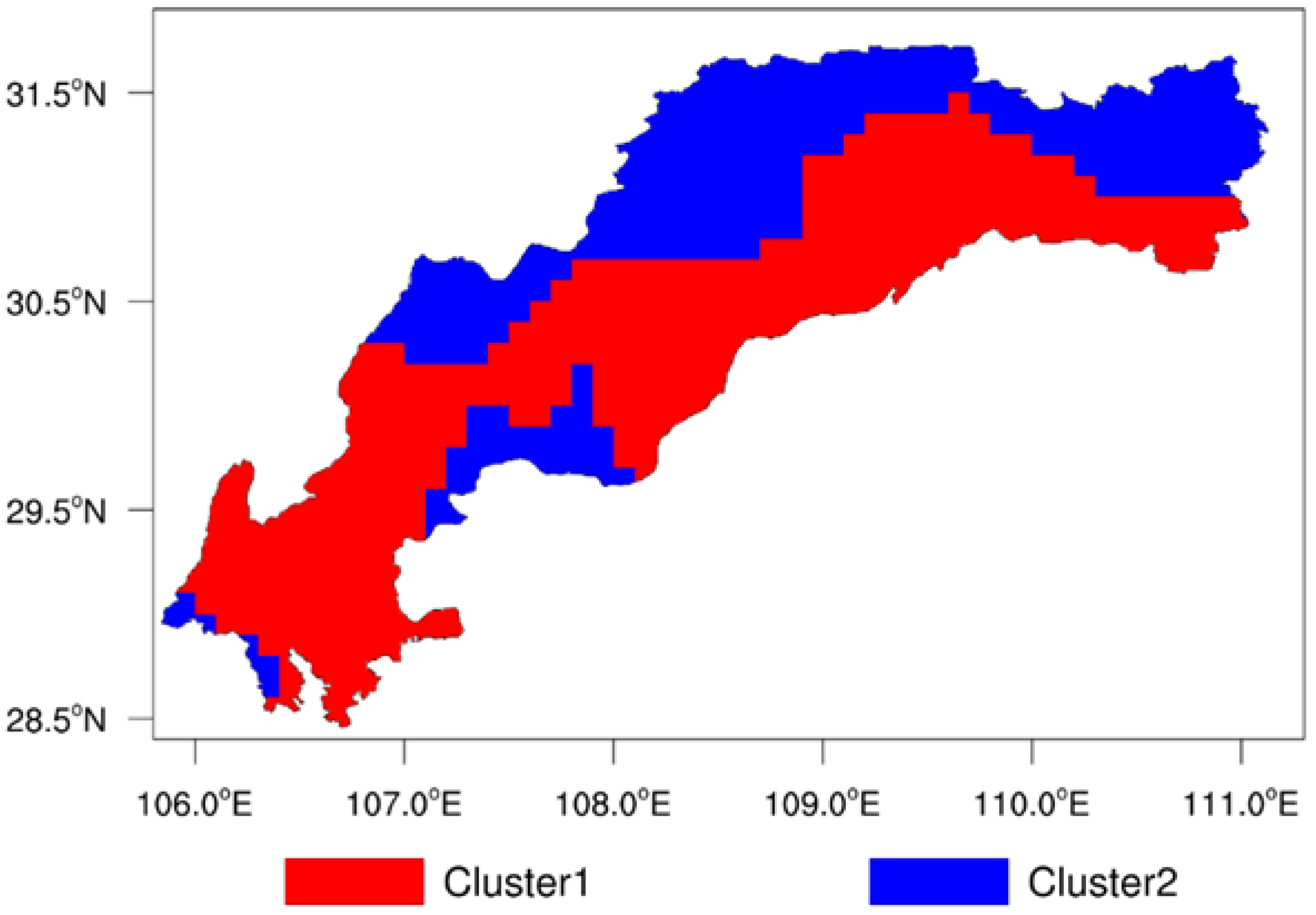
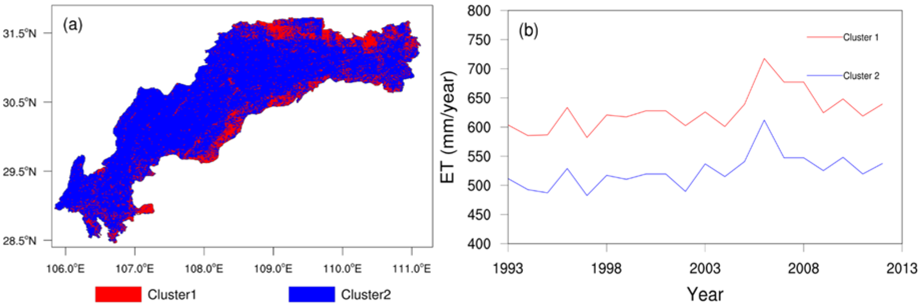
2.3.4. k-Means Clustering Algorithm

The k-means algorithm is a typical distance-based clustering algorithm with simple principle and fast calculation speed [43]. In this paper, this method is used to analyze the variation of ET over the grids with similar climatic conditions. The method assumes that the original data set is {x1, x2, …, xn}, and each xi is a d-dimensional vector. The purpose of k-means clustering is to divide the original data set into k classes S = {S1, S2, …, Sk} for a given number of classifications k (kn). The steps of the k-means algorithm are as follows:
(1)
k data were randomly selected from all data samples as the initial cluster center.
(2)
Calculate the distance of other data to each cluster center and divide them into the nearest cluster.
(3)
The center points of all sample data in each cluster are used to represent each cluster center.
(4)
Repeat steps (2) and (3) until the center point of each cluster is unchanged or reaches the set number of iterations.

3. Results

3.1. Trend in LUCC and Cliamte Change

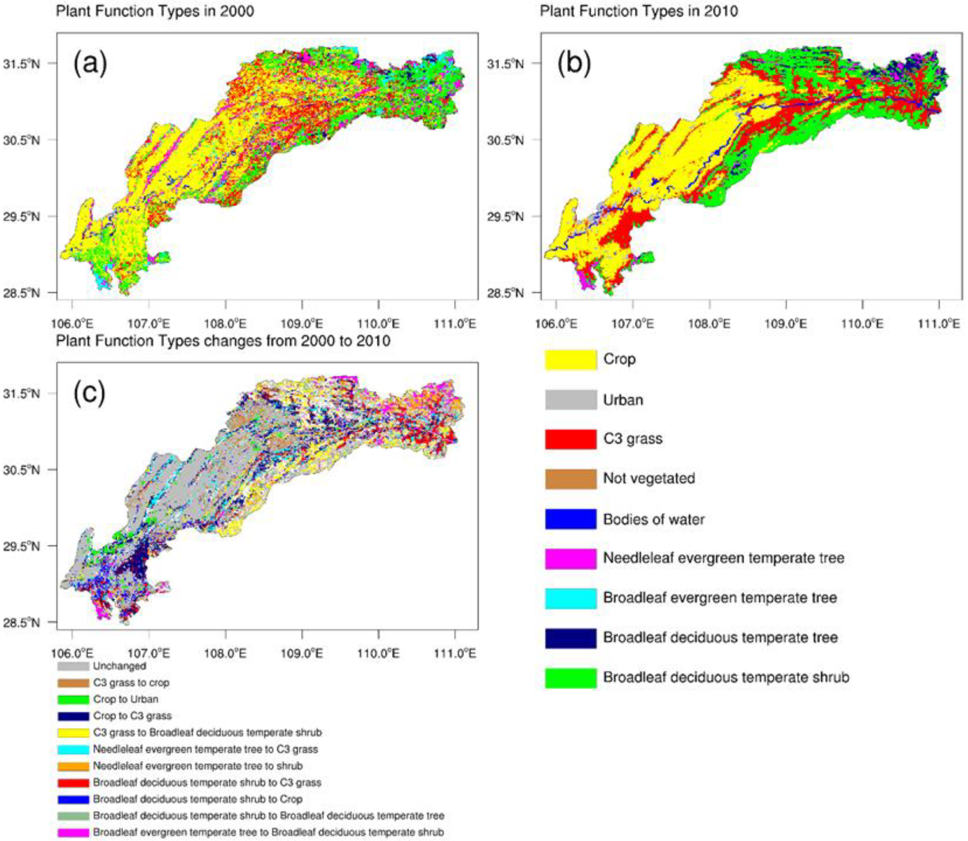
3.1.1. Variation in Land Use/Land Cover

In the CLM4.5 model, the PFTs were used to represent land use/land cover. Figure 2 shows the distribution and conversion of the PFTs in the TGR region in 2000 and 2010. The main PFTs in 2000 were cropland, broadleaf deciduous temperate shrub, C3 grass, and needleleaf evergreen temperate tree. Among them, cropland accounted for the largest proportion (47.41%) and was distributed in flat regions on the left bank of the TGR region. Broadleaf deciduous temperate shrubs accounted for 20.64% and was distributed in the mountainous regions above 1000 m which was at the head and tail of the TGR region. The C3 grass and needleleaf evergreen temperate trees accounted for 15.15% and 8.6%, respectively and were distributed in the mountainous regions at an altitude of 600–1000 m. By 2010, the four main PFTs accounted for 38.86%, 26.65%, 23.42% and 2.48%, respectively. The PFTs had undergone major changes during the past 10 years with cropland decreasing by 8.55%. Resettlement, relocation and supporting facilities for construction were the main reasons for this reduction. During this period, due to the impact of the policy of returning farmland to forests (grass), the ecological environment of the TGR region significantly improved and the cropland continued to decrease. As a result, the forest and grassland increased significantly, with broadleaf deciduous temperate shrubs increasing by 6.01% and C3 grass increasing by 8.27%. The impoundment of the reservoir had inundated some of the vegetation along the river, resulting in an increase in water bodies by 0.51%. At the same time, due to the acceleration of urbanization, the urban areas also increased by 1.92%.

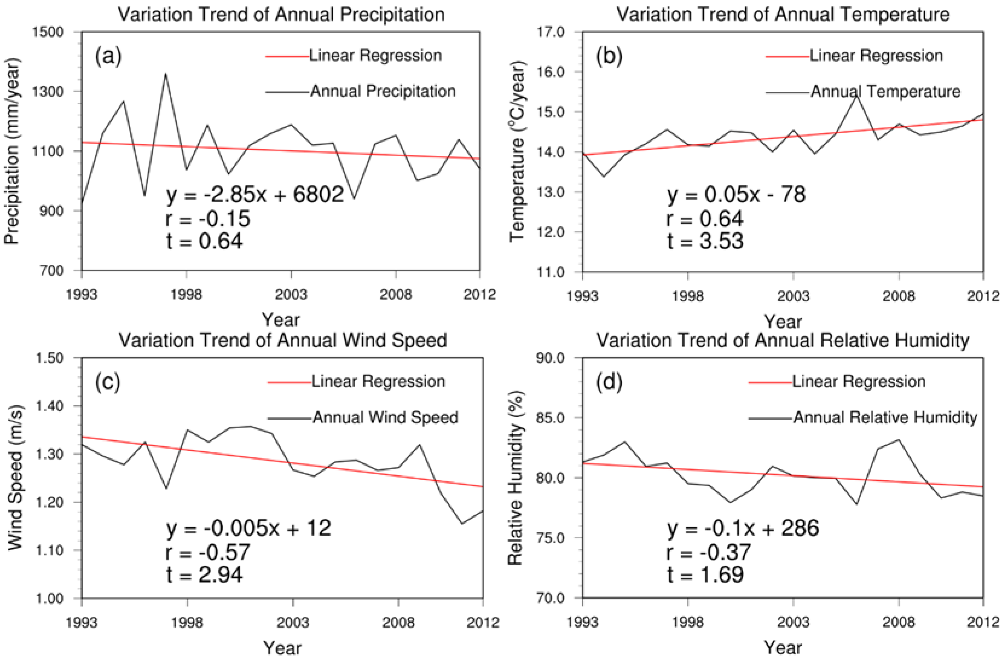
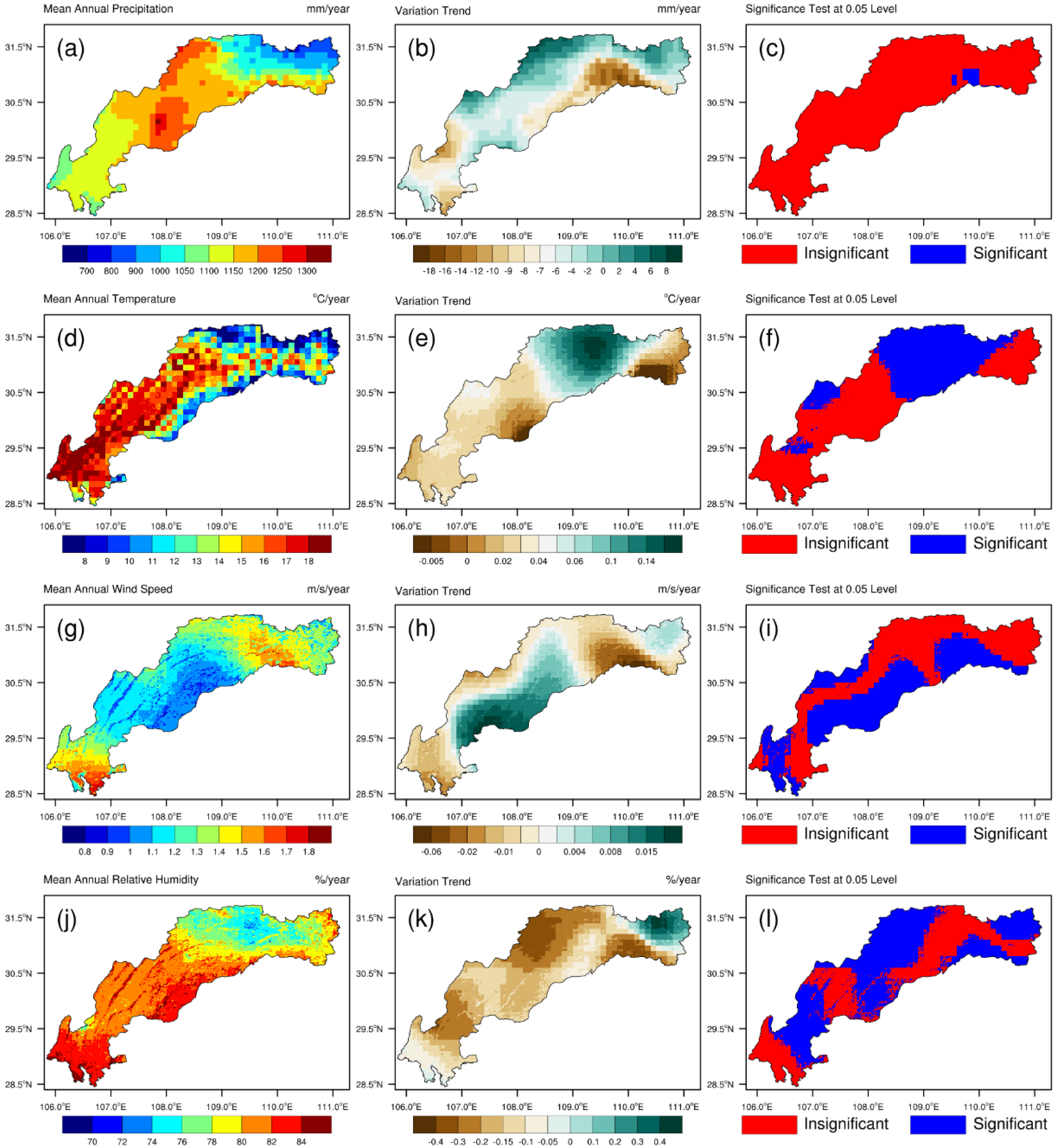
3.1.2. Variation in Climatic Factors

During 1993–2013, the climate in the TGR region showed warming and drying trends on the whole, with spatially averaged changes of 0.05 °C/year for air temperature, 2.85 mm/year for precipitation, −0.005 m/s for wind speed and 0.1%/year for relative humidity (Figure 3). On a monthly scale (Table 2), precipitation showed an increasing trend in spring and a decreasing trend in summer, although, the variations were not statistically significant. The air temperature increased all year round except for January, and this increase was significant in March. The wind speed had been decreasing throughout the year, especially in summer. In addition, the relative humidity also showed a decreasing trend in spring and summer, particularly in March.
Figure 4 shows the spatial distribution characteristics and the variation trend of precipitation, temperature, wind speed and relative humidity in the TGR region from 1993 to 2013. The annual precipitation ranged from 686 to 1306 mm, showing a spatial distribution of greater precipitation in the center and less at the head and tail of the reservoir. Since the construction of the Three Gorges Project, the precipitation showed an increasing trend on the left bank of the reservoir, and a decreasing trend on the right bank, although, the variation trend was not significant. The spatial distribution of the wind speed was opposite to precipitation, with increasing trends observed on the right bank. The spatial distribution of air temperature and relative humidity was relatively consistent, both of which were related to the topography. The air temperature and relative humidity showed an inverse relationship with altitude. The temperatures across the whole region of the reservoir showed an upward trend and increased by more than 0.1 °C/year in the high-altitude mountainous region in the north. This rising trend was clear. The relative humidity of the head of the reservoir showed a significant increasing trend, while other regions showed a decreasing trend, in which the cropland in the center of the reservoir and the urban areas at the tail of the reservoir decreased significantly.
Figure 5 shows the result of the k-means cluster analysis on the variations of precipitation, temperature, wind speed and relative humidity. It was found that dividing the area into two categories can better reflect the variation of the climate. The climate of cluster 1 is characterized by a decreasing trend of precipitation and a significant increasing trend of wind speed, while the climate of cluster 2 is characterized by an increasing trend of precipitation and a significant decreasing trend of relative humidity. The boundary between the two is basically the same as the flow direction of the Yangtze River, which indicates that the climatic conditions are related to the topography and landscape of the basin.

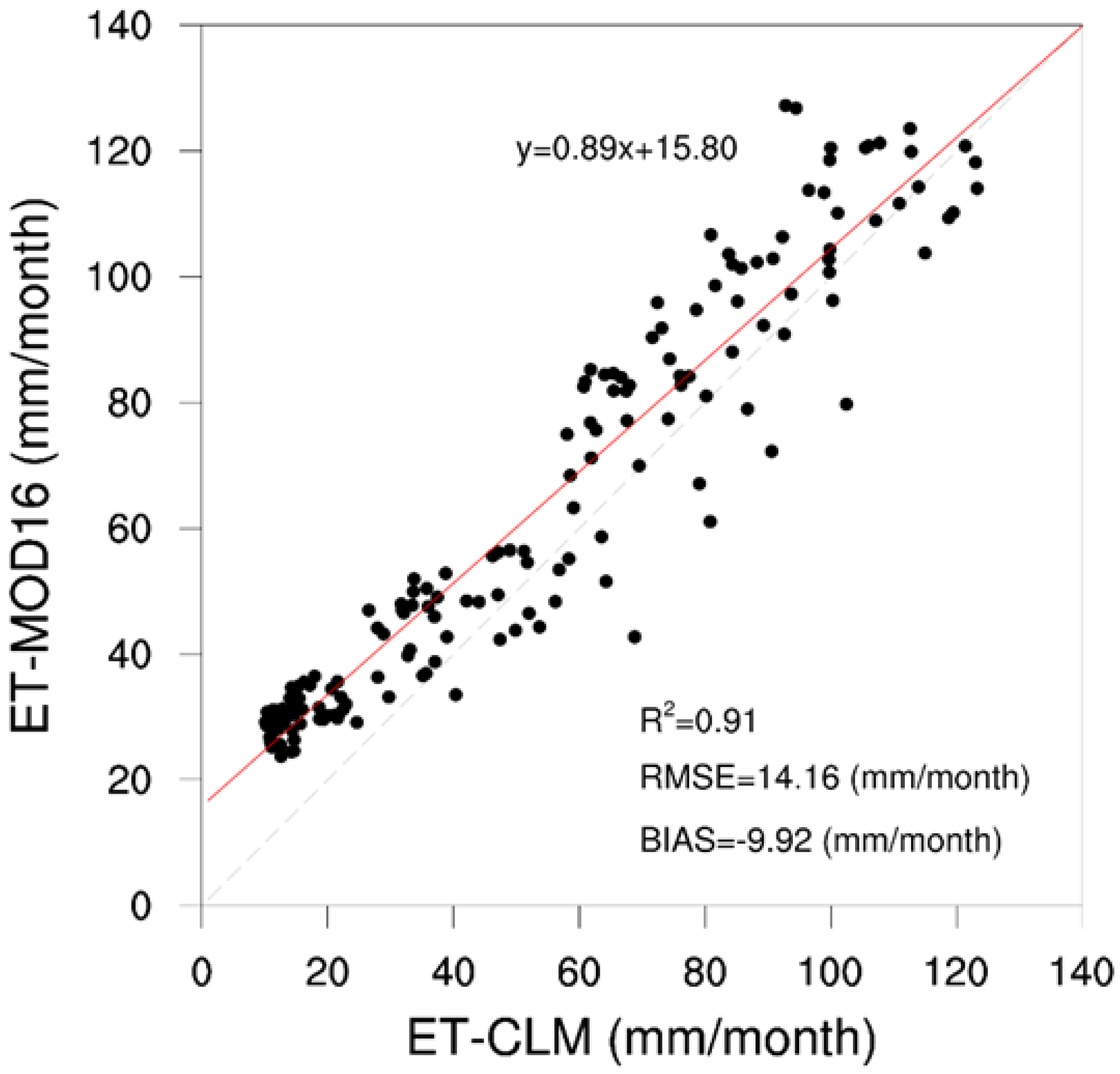
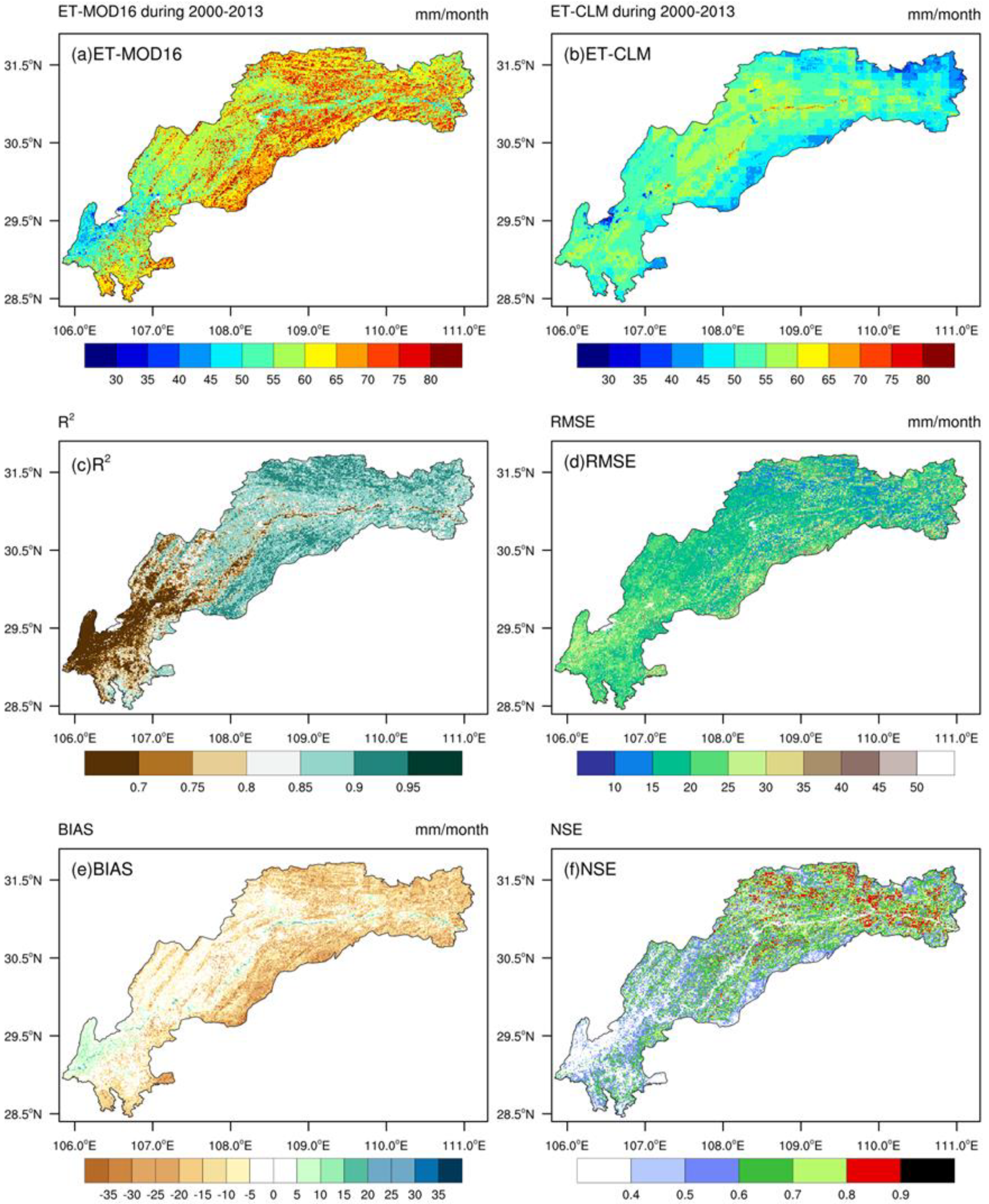
3.2. Model Validation

The data from the MOD16 monthly ET product (ET-MOD16), from 2000 to 2013 was used to validate the results of the CLM. The scatter plot of ET-MOD16 and the corresponding monthly values simulated by CLM 4.5 (ET-CLM) shown in Figure 6, show a good model fit with an R2 which was 0.91, and a regression of y = 0.89x + 15.80. However, most of the scatter points fell above the y = x line, indicating that the CLM model underestimated the simulation of ET in the TGR region. This phenomenon was also confirmed using the BIAS and RMSE values. Furthermore, it was found that the distribution of the scatter points was relatively uniform, indicating that the CLM4.5 model could better reflect the seasonal variation characteristics of ET in the TGR region. However, the underestimation was more prominent among the low values (<40 mm/month), indicating that the simulations performed better in summer than in winter.
In order to analyze the spatial difference between ET-MOD16 and ET-CLM, the monthly mean ET-MOD16 and ET-CLM were calculated from 2000 to 2013, and the four indicators described above were used to evaluate the spatial distribution characteristics. Figure 7 shows that within the TGR region, the BIAS between ET-CLM and ET-MOD16 did not exceed ±35 mm, and was below ±10 mm in the water bodies and cropland on the left bank of the river. The RMSE was consistently less than 30 mm, and less than 15 mm in broadleaf deciduous temperate shrubs in the northern mountainous region, which was better than the urban areas and the cropland (>20 mm). This indicates that the simulation performance on ET of the forest was better than the urban areas and farmland. In addition, it was found that the R2 was less than 0.8 in the urban areas and cropland on the left bank of the river, and the NSE was also less than 0.5 in the same region. The main reason was that the ET-MOD16 only calculated the ET for the vegetated land region based on the Penman-Monteith equation [44], while the value was null for water bodies, barren or sparsely vegetated, permanent wetland, snow and ice, and urban areas. Therefore, on the whole, the CLM4.5 model can better reflect the spatiotemporal distribution characteristics of ET in the TGR region.

3.3. Spatiotemporal Variability of ET

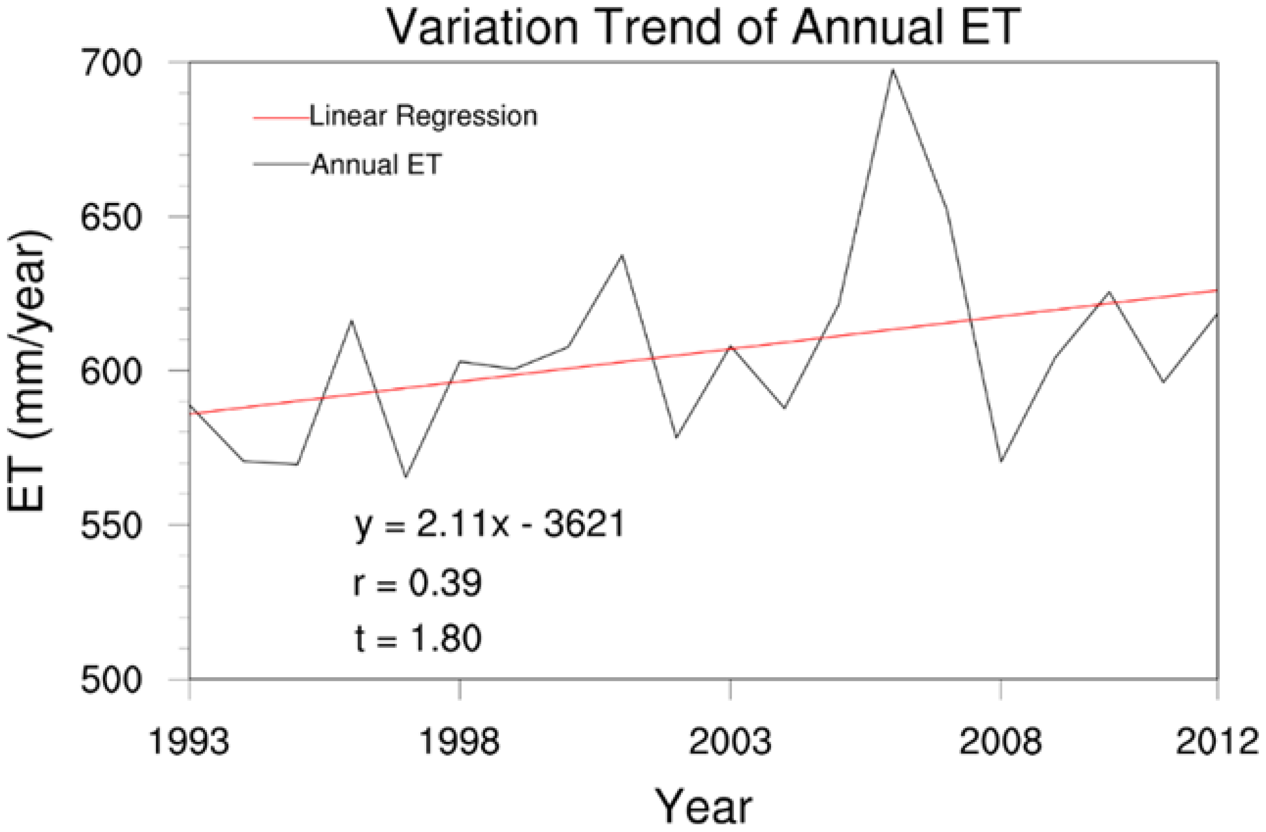
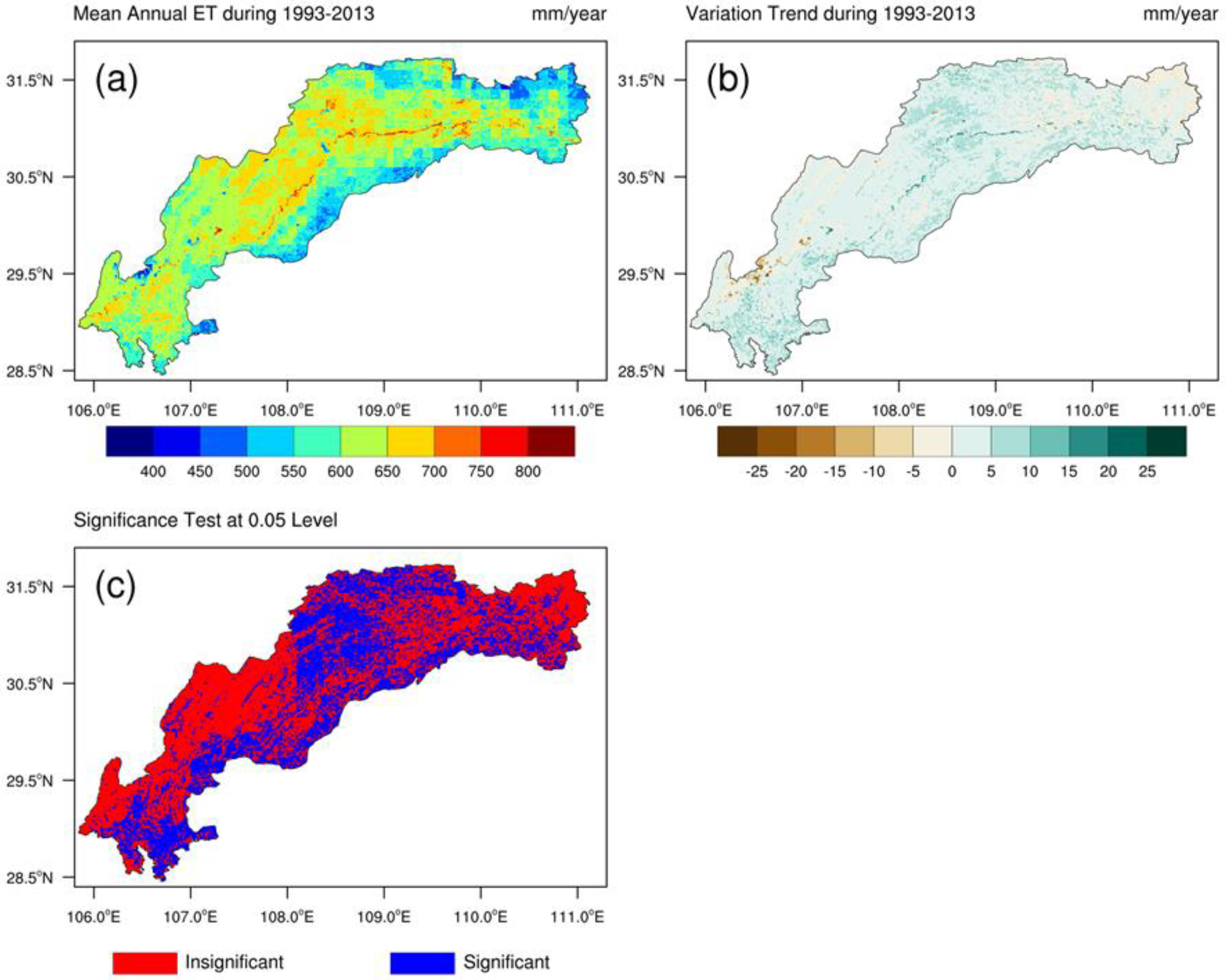
3.3.1. Variation in ET

Figure 8 shows the variation trend of annual ET in the TGR region from 1993 to 2013. The black line indicates the time series of annual ET and the red line shows the linear regression line. The mean annual ET of the TGR region was 606 mm, and the maximum annual ET, which occurred in 2006, was 697 mm. The significant increase in the air temperature was the main reason for the increase in ET. The minimum ET was 565 mm in 1996, the increase in precipitation and the significant decrease in wind speed were the main reasons for the decrease of ET. Over the past 20 years, ET increased at a rate of 2.11 mm/year, although the increasing trend of ET in the TGR region was not significant at the level of 0.05 as the t-test value was equal to 1.80, less than the threshold of 2.086.
Figure 9 shows the spatial distribution characteristics and variation trends of ET in the TGR region during the period 1993–2013. The mean annual ET of the whole area ranged from 350 to 850 mm, among which the ET for the broadleaf deciduous temperate forests was less than 500 mm, while the ET for water bodies was over 700 mm. The ET for urban areas and broadleaf deciduous temperate shrubs in the northern mountainous regions showed a decreasing trend. However, the annual ET in other regions showed an increasing trend ranging from 0 to 25 mm/year. This increasing trend in the high-altitude regions on the right bank of the Yangtze River, and the center of the reservoir was significant (p < 0.05), while the variation trend in other regions was not significant.

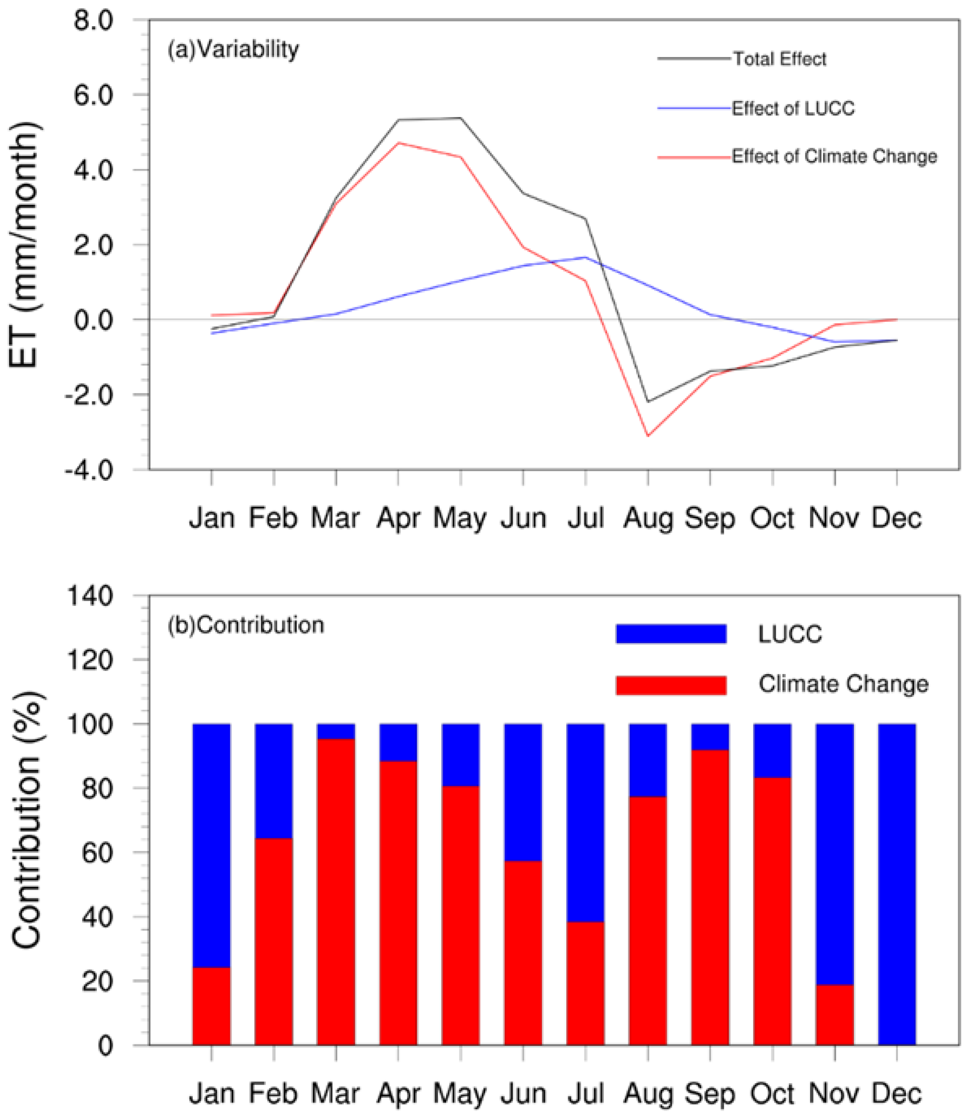
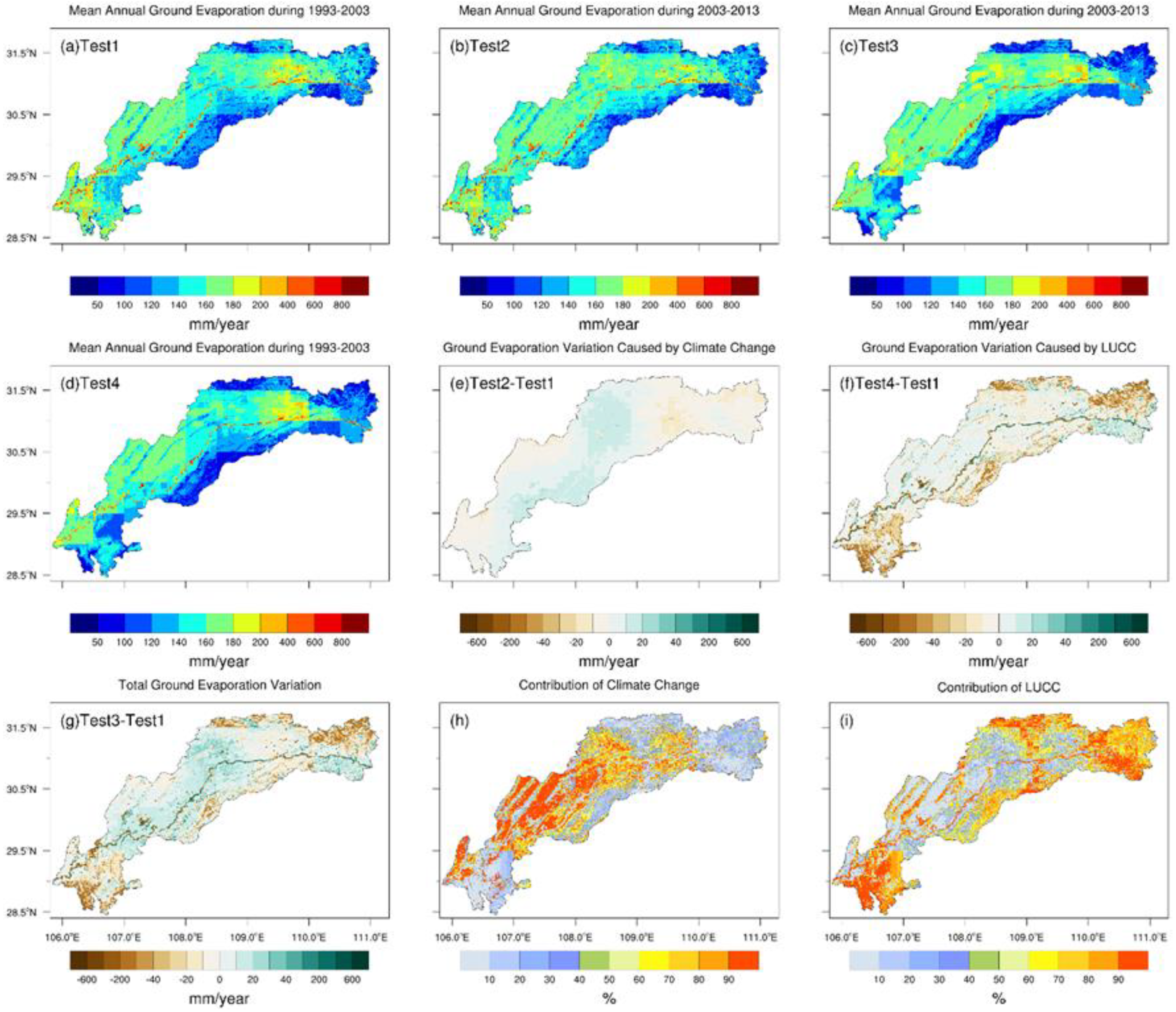
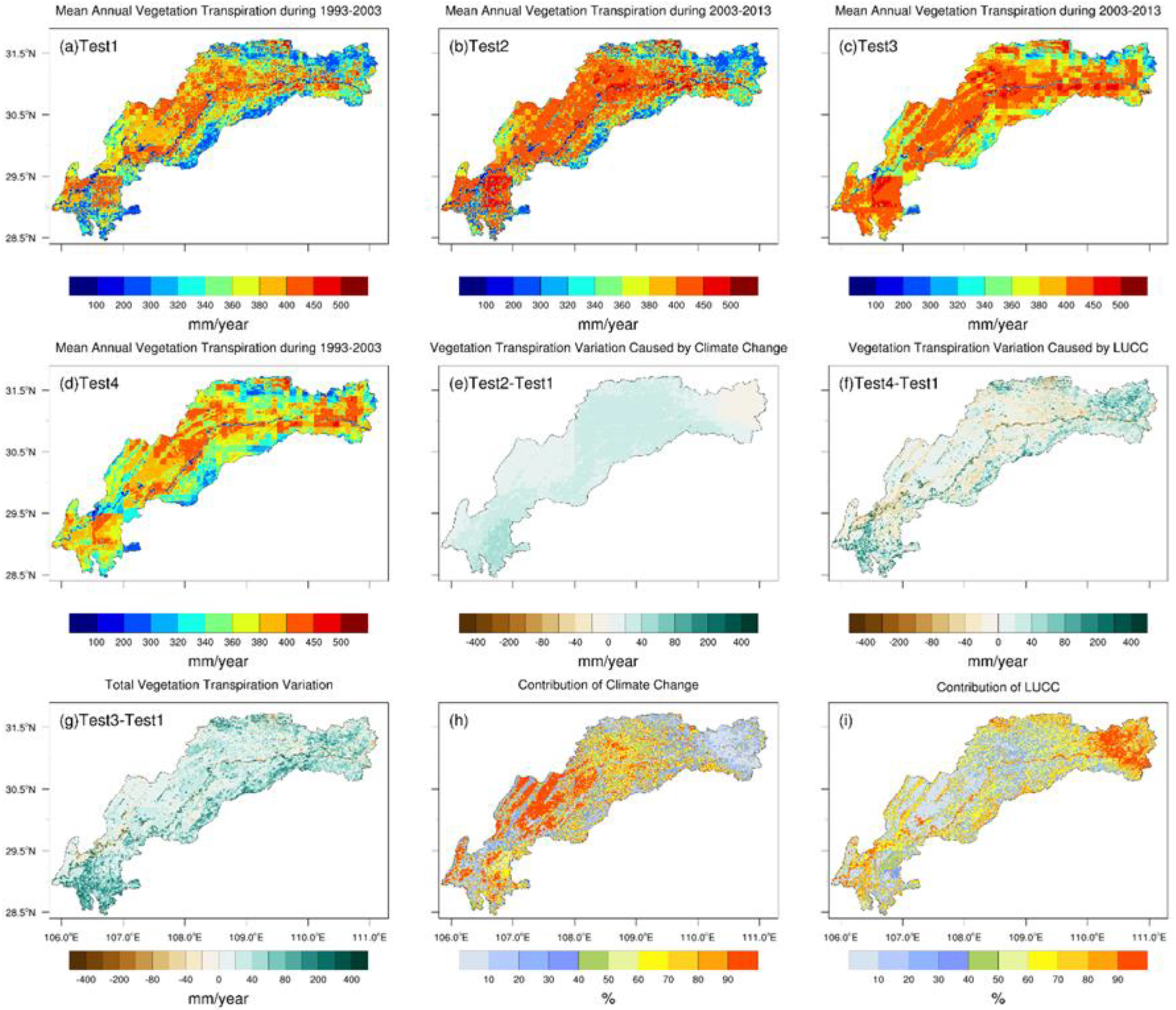
3.3.2. ET Response to Climate Change and LUCC

Figure 10 shows the variation of monthly ET before and after impoundment in the TGR region and the contribution of climate change and LUCC to ET. The mean annual ET increased by 13.76 mm after impoundment, while the increase caused by climate change was 9.61 mm and the increase caused by LUCC was 4.15 mm. In terms of the distributions within a year, ET increased from February to July which was likely caused by climate change, while the increase caused by LUCC occurred from March to September. In general, in the spring, summer, and autumn, climate change was the main factor causing the variability of ET, while LUCC was dominant in the winter.
Figure 11 shows the spatial differences of ET before and after impoundment in the TGR region, as well as the contribution rates of climate change and LUCC to its changes. Figure 11a–d show the mean annual ET for the four tests, and Figure 11e–g indicate the variations in ET before and after impoundment. Figure 11h,i show the contribution rates of climate change and LUCC to ET. Compared with the pre-impoundment period, the mean annual ET in the urban and forest areas at the head of the TGR region was reduced after impoundment, with the mean annual ET in urban areas reduced by more than 200 mm. The reason for this reduction was the increase in hardened pavement caused by the expansion of the city and the reduction of vegetation coverage caused by the conversion of the forests in the northern mountainous regions to grassland. The LUCC had a higher contribution rate to ET variation in these regions and even contributed more than 90% in urban areas. For the center of the TGR region, climate change was the main factor leading to the increase of ET. It could be seen from Figure 4 that the temperature in the region was slightly increasing, the relative humidity was decreasing, and the wind speed was increasing. These factors were all beneficial to the increase of ET.
Figure 12 shows the cluster analysis results of the ET trend. By comparing Figure 5 and Figure 12a, it could be seen that even in places with similar climatic conditions, the trend of ET could be different. Figure 12b shows the variation trend of ET in the two cluster centers. Both cluster 1 and 2 show an increasing trend, and the trends are very similar, but the 3.24 mm/year trend of cluster 1 is higher than the 2.75 mm/year trend of cluster 2. This difference is mainly caused by LUCC, especially from C3 grass to broadleaf deciduous temperate shrubs in high-altitude regions, which can also be confirmed from Figure 11i.

4. Discussion

4.1. Modeling Uncertainties

Although the CLM4.5 model had a good performance in simulating the monthly ET over the TGR region, it is still worthwhile to explore the uncertainties of the modeling results. First, the results showed a slight underestimation of the monthly ET. This underestimation was partly attributed to the limitation that the model does not take the dynamic changes in vegetation into consideration, but used two PFTs in 2000 and 2010 to represent the land use/land cover conditions before and after the impoundment of the TGR region. In the CLM4.5, ET is related to the leaf area index and stem area index. Since dynamic changes in vegetation are not taken into account, the selection of these parameters is uncertain, which affects the simulation results. Secondly, the spatial resolution of the model is 0.01 degree, the time step of the model is 30 min, while the spatial resolution of the atmospheric forcing data is 0.1 degree, and the time resolution is 3 h, which creates uncertainty in the spatio-temporal interpolation. In addition, the TGR is usually dynamically operated according to the upstream inflow, while the CLM4.5 model currently has no reservoir operation module, and cannot reflect the dynamic change of water bodies, which also indirectly affects the variation of PFTs. Therefore, a new module which considers the reservoir operation process and the dynamic changes of vegetation is likely to be developed and a more accurate input dataset is needed to carry out future research.

4.2. Variation in ET Components and Driving Factors

In the CLM4.5 model, ET consists of ground evaporation, canopy evaporation, and vegetation transpiration. An analysis of the variations in these three parts is helpful to understand the variation in total ET. Figure 13, Figure 14 and Figure 15 show the spatial differences of the three parts before and after impoundment in the TGR region, as well as the contribution rates of climate change and LUCC to their changes, respectively. Among the three components, vegetation transpiration accounted for the largest proportion of ET, indicating that most of the ET came from vegetation transpiration. For canopy evaporation, it ranged from 10 to 120 mm. Compared with the pre-impoundment period, the mean annual canopy evaporation in the forest above 1500 m increased after impoundment, while it decreased in other regions, especially urban areas. The increase in vegetation coverage caused by the conversion of grassland to shrubs was the main reason for the increase in canopy evaporation in high altitude regions, and urban expansion was the main reason for the decrease of canopy evaporation in urban areas. Therefore, LUCC was the main factor driving the variation in canopy evaporation in these regions. Ground evaporation ranged from 50 to 800 mm. As water bodies were not covered by vegetation, their ground evaporation was higher, which almost equaled to their potential ET. The variation in ground evaporation is consistent with total ET. The vegetation transpiration ranged from 100 to 500 mm. The impounding of the TGR made the water table rise and inundated parts of the vegetation along the river, resulting in a reduction of vegetation transpiration in these water bodies. Apart from a small part of the head of the TGR region, the relative humidity in other regions showed a decreasing trend, and the decrease was significant in most areas in the center of the TGR region. The decrease in relative humidity led to an increase in the degree of stomatal opening, which in turn increased the transpiration rate. Therefore, climate change was the main factor for the increase of vegetation transpiration in most areas of the TGR region. Overall, the total ET increased after impoundment in the TGR region. The ET and its components presented different spatial characteristics which were affected to different degrees by climate change and LUCC.

5. Conclusions

A CLM4.5 land surface model was used to assess the impact of climate change and LUCC on ET in the TGR region before and after impoundment. Four experiments were conducted to analyze the spatial and temporal distribution and the variation trend of ET and climatic factors as well as the contribution of climate change and LUCC to ET. The following conclusions can be reached:
(1)
During 1993–2013, the TGR region had witnessed a warm and dry climate trend with the decrease of precipitation, wind speed and relative humidity and the increase in temperature. At the same time, the construction of the TGR region and the implementation of the policy of returning farmland to forests (grass) led to a reduction in cropland and an increase in forests, grasslands, water bodies and urban areas. In this context, the mean annual ET of the TGR region increased at a rate of 2.11 mm/year.
(2)
The CLM4.5 land surface model was suitable to model the ET in the TGR region. The results from the four evaluation indexes showed that the CLM4.5 model slightly underestimated the ET of the TGR region. It is, therefore, highly recommended that a new module considering the reservoir operation process and the dynamic changes of vegetation should be integrated into the CLM4.5 model and more precise data should be used in the future to improve the accuracy of the simulation performance.
(3)
The cluster analysis showed that two categories can better reflect the climatic conditions of TGR. The ET of similar climatic conditions is not necessarily similar, and LUCC can also affect ET. The LUCC in high altitude regions make the cluster analysis results of ET significantly different from other regions.
(4)
The mean annual ET of the TGR was 606 mm which increased by 13.76 mm after impoundment. The increase due to climate change was 9.61 mm, while the increase due to LUCC was 4.15 mm. Spatially, vegetation transpiration accounted for the largest proportion of ET. The decrease in relative humidity was the most important factor for the increase in vegetation transpiration, while the increase in ground evaporation was primarily due to the increase in wind speed in the center of the TGR region. The change in the PFTs, caused by urbanization and the construction of the TGR region, was the main factor causing the variation in ET in the water bodies, urban areas and high-altitude regions of the TGR region. These combined effects led to the increase in ET after impoundment and showed different spatial distribution characteristics in the TGR region.

Author Contributions

Conceptualization, H.W. and W.X.; methodology, Y.Z. (Yong Zhao) and Y.W.; software, H.W. and B.H.; validation, X.Z.; formal analysis, Y.Z. (Yuyan Zhou); resources, H.Y.; data curation, H.C.; writing—original draft preparation, H.W.; writing—review and editing, W.X.; visualization, H.C.

Funding

This research was funded by the National Key Research and Development Program during the 13th Five-Year Plan, grant number 2017YFC0404701; the National Natural Science Foundation of China, grant number 51779271 and the International S&T Cooperation Program of China, grant number 2016YFE0102400.

Acknowledgments

The authors are grateful to the colleagues in National SuperComputer Center in Tianjin for their help in running and modifying the CLM4.5 model.

Conflicts of Interest

The authors declare no conflict of interest.

References

  1. Jung, M.; Reichstein, M.; Ciais, P.; Seneviratne, S.I.; Sheffield, J.; Goulden, M.L.; Bonan, G.; Cescatti, A.; Chen, J.Q.; de Jeu, R.; et al. Recent decline in the global land evapotranspiration trend due to limited moisture supply. Nature 2010, 467, 951–954. [Google Scholar] [CrossRef] [PubMed]
  2. Vörösmarty, C.J.; Green, P.; Salisbury, J.; Lammers, R.B. Global water resources: Vulnerability from climate change and population growth. Science 2000, 289, 284–288. [Google Scholar]
  3. Shukla, J.; Mintz, Y. Influence of Land-Surface Evapotranspiration on the Earth’s Climate. Science 1982, 215, 1498–1501. [Google Scholar] [CrossRef]
  4. Pan, S.F.; Tian, H.Q.; Dangal, S.R.; Yang, Q.C.; Yang, J.; Lu, C.Q.; Tao, B.; Ren, W.; Ouyang, Z.Y. Response of global terrestrial evapotranspiration to climate change and increasing atmospheric CO2 in the 21st century. Earth’s Future 2015, 3, 15–35. [Google Scholar] [CrossRef]
  5. Mononen, L.; Auvinen, A.P.; Ahokumpu, A.L.; Rönkä, M.; Aarras, N.; Tolvanen, H.; Kamppinen, M.; Viirret, E.; Kumpula, T.; Vihervaara, P. National ecosystem service indicators: Measures of social-ecological sustainability. Ecol. Indic. 2016, 61, 27–37. [Google Scholar] [CrossRef]
  6. Tang, Q.; Bao, Y.H.; He, X.B.; Fu, B.J.; Collins, A.L.; Zhang, X.B. Flow regulation manipulates contemporary seasonal sedimentary dynamics in the reservoir fluctuation zone of the Three Gorges Reservoir, China. Sci. Total Environ. 2016, 548, 410–420. [Google Scholar] [CrossRef]
  7. Huang, C.B.; Huang, X.; Peng, C.H.; Zhou, Z.X.; Teng, M.J.; Wang, P.C. Land use/cover change in the Three Gorges Reservoir area, China: Reconciling the land use conflicts between development and protection. Catena 2019, 175, 388–399. [Google Scholar] [CrossRef]
  8. Reder, A.; Rianna, G.; Vezzoli, R.; Mercogliano, P. Assessment of possible impacts of climate change on the hydrological regimes of different regions in China. Adv. Clim. Chang. Res. 2016, 7, 169–184. [Google Scholar] [CrossRef]
  9. Huo, Z.L.; Dai, X.Q.; Feng, S.Y.; Kang, S.Z.; Huang, G.H. Effect of climate change on reference evapotranspiration and aridity index in arid region of China. J. Hydrol. 2013, 492, 24–34. [Google Scholar] [CrossRef]
  10. Gong, L.B.; Xu, C.Y.; Chen, D.L.; Halldin, S.; Chen, Y.D. Sensitivity of the Penman-Monteith reference evapotranspiration to key climatic variables in the Changjiang (Yangtze River) basin. J. Hydrol. 2006, 329, 620–629. [Google Scholar] [CrossRef]
  11. Xu, C.Y.; Gong, L.B.; Jiang, T.; Chen, D.L.; Singh, V.P. Analysis of spatial distribution and temporal trend of reference evapotranspiration and pan evaporation in Changjiang (Yangtze River) catchment. J. Hydrol. 2006, 327, 81–93. [Google Scholar] [CrossRef]
  12. Fan, J.L.; Wu, L.F.; Zhang, F.C.; Xiang, Y.Z.; Zheng, J. Climate change effects on reference crop evapotranspiration across different climatic zones of China during 1956-2015. J. Hydrol. 2016, 542, 923–937. [Google Scholar] [CrossRef]
  13. Bosch, J.M.; Hewlett, J.D. A review of catchment experiments to determine the effect of vegetation changes on water yield and evapotranspiration. J. Hydrol. 1982, 55, 3–23. [Google Scholar] [CrossRef]
  14. Gao, G.; Chen, D.L.; Xu, C.Y.; Simelton, E. Trend of estimated actual evapotranspiration over China during 1960-2002. J. Geophys. Res. 2007, 112, D11120. [Google Scholar] [CrossRef]
  15. French, A.N.; Hunsaker, D.J.; Thorp, K.R. Remote sensing of evapotranspiration over cotton using the TSEB and METRIC energy balance models. Remote Sens. Environ. 2015, 158, 281–294. [Google Scholar] [CrossRef]
  16. Liu, M.L.; Tian, H.Q.; Chen, G.S.; Ren, W.; Zhang, C.; Liu, J.Y. Effects of land-use and land-cover change on evapotranspiration and water yield in China during 1900-2000. J. Am. Water Resour. Assoc. 2008, 44, 1193–1207. [Google Scholar] [CrossRef]
  17. Olchev, A.; Ibrom, A.; Priess, J.; Erasmi, S.; Leemhuis, C.; Twele, A.; Radler, K.; Kreilein, H.; Panferov, O.; Gravenhorst, G. Effects of land-use changes on evapotranspiration of tropical rain forest margin area in Central Sulawesi (Indonesia): Modelling study with a regional SVAT model. Ecol. Model. 2008, 212, 131–137. [Google Scholar] [CrossRef]
  18. Tian, H.Q.; Chen, G.S.; Liu, M.L.; Zhang, C.; Sun, G.; Lu, C.Q.; Xu, X.F.; Ren, W.; Pan, S.F.; Chappelka, A. Model estimates of net primary productivity, evapotranspiration, and water use efficiency in the terrestrial ecosystems of the southern United States during 1895–2007. For. Ecol. Manag. 2010, 259, 1311–1327. [Google Scholar] [CrossRef]
  19. Wang, K.C.; Dickinson, R.E. A review of global terrestrial evapotranspiration: Observation, modeling, climatology, and climatic variability. Rev. Geophys. 2012, 50, RG2005. [Google Scholar]
  20. Zhang, L.; Nan, Z.T.; Yu, W.J.; Zhao, Y.B.; Xu, Y. Comparison of baseline period choices for separating climate and land use/land cover change impacts on watershed hydrology using distributed hydrological models. Sci. Total Environ. 2018, 622–623, 1016–1028. [Google Scholar] [CrossRef] [PubMed]
  21. Bai, M.; Mo, X.G.; Liu, S.X.; Hu, S. Contributions of climate change and vegetation greening to evapotranspiration trend in a typical hilly-gully basin on the Loess Plateau, China. Sci. Total Environ. 2019, 657, 325–339. [Google Scholar] [CrossRef] [PubMed]
  22. Yuan, W.P.; Liu, S.G.; Yu, G.R.; Bonnefond, J.M.; Chen, J.Q.; Davis, K.; Desai, A.R.; Goldstein, A.H.; Gianelle, D.; Rossi, F.; et al. Global estimates of evapotranspiration and gross primary production based on MODIS and global meteorology data. Remote Sens. Environ. 2010, 114, 1416–1431. [Google Scholar] [CrossRef] [Green Version]
  23. Stoy, P.C.; Katul, G.G.; Siqueira, M.B.; Juang, J.Y.; Novick, K.A.; McCarthy, H.R.; Oishi, A.C.; Uebelherr, J.M.; Kim, H.S.; Oren, R. Separating the effects of climate and vegetation on evapotranspiration along a successional chronosequence in the southeastern US. Glob. Chang. Biol. 2006, 12, 2115–2135. [Google Scholar] [CrossRef] [Green Version]
  24. Li, G.; Zhang, F.M.; Jing, Y.S.; Liu, Y.B.; Sun, G. Response of evapotranspiration to changes in land use and land cover and climate in China during 2001-2013. Sci. Total Environ. 2017, 596–597, 256–265. [Google Scholar] [CrossRef] [PubMed]
  25. Chen, Y.Y.; Yang, K.; He, J.; Qin, J.; Shi, J.C.; Du, J.Y.; He, Q. Improving land surface temperature modeling for dry land of China. J. Geophys. Res. 2011, 116, D20104. [Google Scholar] [CrossRef]
  26. Yang, K.; He, J.; Tang, W.J.; Qin, J.; Cheng, C.C. On downward shortwave and longwave radiations over high altitude regions: Observation and modeling in the Tibetan Plateau. Agric. For. Meteorol. 2010, 150, 38–46. [Google Scholar] [CrossRef]
  27. Ran, Y.H.; Li, X.; Lu, L.; Li, Z.Y. Large-scale land cover mapping with the integration of multi-source information based on the Dempster-Shafer theory. Int. J. Geogr. Inf. Sci. 2011, 26, 169–191. [Google Scholar] [CrossRef]
  28. Friedl, M.A.; McIver, D.K.; Hodges, J.C.; Zhang, X.Y.; Muchoney, D.; Strahler, A.H.; Woodcock, C.E.; Gopal, S.; Schneider, A.; Cooper, A.; et al. Global land cover mapping from MODIS: Algorithms and early results. Remote Sens. Environ. 2002, 83, 287–302. [Google Scholar] [CrossRef]
  29. Friedl, M.A.; Sulla-Menashe, D.; Tan, B.; Schneider, A.; Ramankutty, N.; Sibley, A.; Huang, X.M. MODIS Collection 5 global land cover: Algorithm refinements and characterization of new datasets. Remote Sens. Environ. 2010, 114, 168–182. [Google Scholar] [CrossRef]
  30. Bonan, G.B.; Levis, S.; Kergoat, L.; Oleson, K.W. Landscapes as patches of plant functional types: An integrating concept for climate and ecosystem model. Glob. Biogeochem. Cycles 2002, 16, 5-1–5-23. [Google Scholar] [CrossRef]
  31. Shangguan, W.; Dai, Y.J.; Liu, B.Y.; Zhu, A.X.; Duan, Q.Y.; Wu, L.Z.; Ji, D.Y.; Ye, A.Z.; Yuan, H.; Zhang, Q.; et al. A China data set of soil properties for land surface modeling. J. Adv. Model. Earth Syst. 2013, 5, 212–224. [Google Scholar] [CrossRef]
  32. Mu, Q.Z.; Heinsch, F.A.; Zhao, M.S.; Running, S.W. Development of a global evapotranspiration algorithm based on MODIS and global meteorology data. Remote Sens. Environ. 2007, 111, 519–536. [Google Scholar] [CrossRef]
  33. Mu, Q.Z.; Zhao, M.S.; Running, S.W. Improvements to a MODIS global terrestrial evapotranspiration algorithm. Remote Sens. Environ. 2011, 115, 1781–1800. [Google Scholar] [CrossRef]
  34. Oleson, K.; Lawrence, D.; Bonan, G.; Drewniak, B.; Huang, M.; Koven, C.; Levis, S.; Li, F.; Riley, W.; Subin, Z.; et al. Technical Description of Version 4.5 of the Community Land Model (CLM), 1st ed.; National Center for Atmospheric Research: Boulder, CO, USA, 2013; pp. 1–11. [Google Scholar]
  35. Hurrell, J.W.; Holland, M.M.; Gent, P.R.; Ghan, S.; Kay, J.E.; Kushner, P.J.; Lamarque, J.F.; Large, W.G.; Lawrence, D.; Lindsay, K.; et al. The community earth system model: A framework for collaborative research. Bull. Am. Meteorol. Soc. 2013, 94, 1339–1360. [Google Scholar] [CrossRef]
  36. Lindsay, K.; Bonan, G.B.; Doney, S.C.; Hoffman, F.M.; Lawrence, D.M.; Long, M.C.; Mahowald, N.M.; Moore, J.K.; Randerson, J.T.; Thornton, P.E. Preindustrial-control and twentieth-century carbon cycle experiments with the earth system model CESM1 (BGC). J. Clim. 2014, 27, 8981–9005. [Google Scholar] [CrossRef]
  37. Jia, B.H.; Wang, Y.Y.; Xie, Z.H. Responses of the terrestrial carbon cycle to drought over China: Modeling sensitivities of the interactive nitrogen and dynamic vegetation. Ecol. Model. 2018, 368, 52–68. [Google Scholar] [CrossRef]
  38. Lawrence, D.M.; Thornton, P.E.; Oleson, K.W.; Bonan, G.B. The partitioning of evapotranspiration into transpiration, soil evaporation, and canopy evaporation in a GCM: Impacts on land-atmosphere interaction. J. Hydrometeorol. 2007, 8, 862–880. [Google Scholar] [CrossRef]
  39. Kool, D.; Agam, N.; Lazarovitch, N.; Heitman, J.L.; Sauer, T.J.; Ben-Gal, A. A review of approaches for evapotranspiration partitioning. Agric. For. Meteorol. 2014, 184, 56–70. [Google Scholar] [CrossRef]
  40. Nash, J.E.; Sutcliffe, J.V. River flow forecasting through conceptual models part I–A discussion of principles. J. Hydrol. 1970, 10, 282–290. [Google Scholar] [CrossRef]
  41. Gupta, H.V.; Sorooshian, S.; Yapo, P.O. Status of automatic calibration for hydrologic models: Comparison with multilevel expert calibration. J. Hydrol. Eng. 1999, 4, 135–143. [Google Scholar] [CrossRef]
  42. Box, J.F. Guinness, Gosset, Fisher, and small samples. Stat. Sci. 1987, 2, 45–52. [Google Scholar] [CrossRef]
  43. MacQueen, J. Some methods for classification and analysis of multivariate observations. Proceedings of Berkeley Symposium on Mathematical Statistics Probability, Berkeley, CA, USA, 21 June 1967. [Google Scholar]
  44. Monteith, J. Evaporation and the Environment, 1st ed.; Cambridge University Press: Cambridge, UK, 1965; pp. 205–234. [Google Scholar]
Figure 1. Study area and location of the Three Gorges Reservoir (TGR) region in the Yangtze River Basin.
Water 11 01739 g001
Figure 2. The plant function types (PFTs) and their conversion from 2000 to 2010.
Water 11 01739 g002
Figure 3. The variation trend of annual climatic factors from 1993 to 2013.
Water 11 01739 g003
Figure 4. The spatial distribution and variation trends of annual climatic factors.
Water 11 01739 g004
Figure 5. Cluster analysis results of meteorological factors.
Water 11 01739 g005
Figure 6. Scatter plot of ET-MOD16 and ET-CLM.
Water 11 01739 g006
Figure 7. The spatial distribution of ET-MOD16 and ET-CLM and their evaluation indicators.
Water 11 01739 g007
Figure 8. The variation trend of annual evapotranspiration (ET) from 1993 to 2012.
Water 11 01739 g008
Figure 9. The spatial distribution and variation trend of annual ET.
Water 11 01739 g009
Figure 10. The fluctuations in the effects of climate change and land use/land cover (LUCC) on ET.
Water 11 01739 g010
Figure 11. The spatial differences and the contribution of climate change and LUCC to total ET before and after impoundment.
Water 11 01739 g011
Figure 12. Cluster analysis results of the ET trend. (a) Spatial distribution of cluster of the ET trend; (b) Time series of annual ET of each cluster.
Water 11 01739 g012
Figure 13. The spatial differences and the contribution of climate change and LUCC to canopy evaporation before and after impoundment.
Water 11 01739 g013
Figure 14. The spatial differences and the contribution of climate change and LUCC to ground evaporation before and after impoundment.
Water 11 01739 g014
Figure 15. The spatial differences and the contribution of climate change and LUCC to vegetation transpiration before and after impoundment.
Water 11 01739 g015
Table 1. The description of constructed simulation tests.
TestAtmospheric ForcingLand Use/Land Cover
Test 1June 1993–May 20032000
Test 2June 2003–May 20132000
Test 3June 2003–May 20132010
Test 4June 1993–May 20032010
Table 2. The inter-annual variation trend of monthly climatic factors from 1993 to 2013.
Climatic FactorsJanFebMarAprMayJunJulAugSepOctNovDec
P(mm·a−1)−0.150.020.670.201.03−2.39−3.310.322.41−1.670.47−0.43
T(°C·a−1)−0.0050.0580.105 *10.0620.0590.0400.0550.0310.0490.0570.0350.011
W(m·s−1·a−1)−0.003−0.002−0.007−0.009−0.003−0.009 *−0.006 *−0.010 *−0.005−0.007 *−0.004−0.0004
RH(%·a−1)−0.23 *0.003−0.24 *−0.18−0.09−0.09−0.13−0.07−0.07−0.0030.02−0.16
1 Significance level: * (p < 0.05).

