Machine Learning Approaches to Develop Pedotransfer Functions for Tropical Sri Lankan Soils
by
 ,
,
M.H.J.P. Gunarathna
1,2,* ,
,
Kazuhito Sakai
3,*, 
Tamotsu Nakandakari
3,
Kazuro Momii
4 and
M.K.N. Kumari
1,2 1
United Graduate School of Agricultural Sciences, Kagoshima University, 1-21-24 Korimoto, Kagoshima-shi, Kagoshima 890-0065, Japan
2
Faculty of Agriculture, Rajarata University of Sri Lanka, Puliyankulama, Anuradhapura 50000, Sri Lanka
3
Faculty of Agriculture, University of the Ryukyus, 1 Senbaru, Nishihara-cho, Okinawa 903-0213, Japan
4
Faculty of Agriculture, Kagoshima University, 1-21-24 Korimoto, Kagoshima-shi, Kagoshima 890-8580, Japan
*
Authors to whom correspondence should be addressed.
Water 2019, 11(9), 1940; https://doi.org/10.3390/w11091940
Submission received: 8 July 2019
/
Revised: 15 September 2019
/
Accepted: 16 September 2019
/
Published: 18 September 2019
(This article belongs to the Section Water, Agriculture and Aquaculture)
Abstract
:Poor data availability on soil hydraulic properties in tropical regions hampers many studies, including crop and environmental modeling. The high cost and effort of measurement and the increasing demand for such data have driven researchers to search for alternative approaches. Pedotransfer functions (PTFs) are predictive functions used to estimate soil properties by easily measurable soil parameters. PTFs are popular in temperate regions, but few attempts have been made to develop PTFs in tropical regions. Regression approaches are widely used to develop PTFs worldwide, and recently a few attempts were made using machine learning methods. PTFs for tropical Sri Lankan soils have already been developed using classical multiple linear regression approaches. However, no attempts were made to use machine learning approaches. This study aimed to determine the applicability of machine learning algorithms in developing PTFs for tropical Sri Lankan soils. We tested three machine learning algorithms (artificial neural networks (ANN), k-nearest neighbor (KNN), and random forest (RF)) with three different input combination (sand, silt, and clay (SSC) percentages; SSC and bulk density (BD); SSC, BD, and organic carbon (OC)) to estimate volumetric water content (VWC) at −10 kPa, −33 kPa (representing field capacity (FC); however, most studies in Sri Lanka use −33 kPa as the FC) and −1500 kPa (representing the permanent wilting point (PWP)) of Sri Lankan soils. This analysis used the open-source data mining software in the Waikato Environment for Knowledge Analysis. Using a wrapper approach and best-first search method, we selected the most appropriate inputs to develop PTFs using different machine learning algorithms and input levels. We developed PTFs to estimate FC and PWP and compared them with the previously reported PTFs for tropical Sri Lankan soils. We found that RF was the best algorithm to develop PTFs for tropical Sri Lankan soils. We tried to further the development of PTFs by adding volumetric water content at −10 kPa as an input variable because it is quite an easily measurable parameter compared to the other targeted VWCs. With the addition of VWC at −10 kPa, all machine learning algorithms boosted the performance. However, RF was the best. We studied the functionality of finetuned PTFs and found that they can estimate the available water content of Sri Lankan soils as well as measurements-based calculations. We identified RF as a robust alternative to linear regression methods in developing PTFs to estimate field capacity and the permanent wilting point of tropical Sri Lankan soils. With those findings, we recommended that PTFs be developed using the RF algorithm in the related software to make up for the data gaps present in tropical regions.
1. Introduction
Data on soil hydraulic properties are increasingly used due to the popularization of agricultural automation and the use of models that support modern agriculture [1]. However, direct measurement of soil hydraulic properties is laborious, costly, and time-consuming [2,3], so the development of inexpensive, rapid, alternative methods to estimate those properties is an area of active research [1,4].
Pedotransfer functions (PTFs) are predictive functions used to estimate difficult-to-measure soil parameters by easily measurable soil parameters [5,6]. Point-based PTFs are used to estimate soil parameters at specific values of matric potential [1,6]. The soil moisture content at −10 and −33 kPa (representing field capacity) and moisture content at −1500 kPa (representing permanent wilting point) are the standard reference values used to develop point PTFs [1,7]. Point-based PTFs have mainly been developed by regression approaches [8]. During the last few decades, regression approaches have been successfully used to develop PTFs to estimate specific points on the moisture retention curve [2,6,9,10,11]. Recently, machine learning approaches have been used in PTF development, such as the k-nearest neighbor (KNN) [10,12], artificial neural networks (ANN) [13,14,15], and random forests (RF) approaches [16,17]. However, despite the frequent application in hydrological/hydrogeological research [18,19,20,21,22,23,24,25], machine learning approaches are still hardly used to develop PTFs.
The advantages of different models vary depending on their complexity [2]. Linear models offer ease of use, parsimony, interpretability, and computational efficiency [6], whereas RF models offer robustness against input outliers, the ability to compensate for irrelevant inputs, and predictive power [26]. One study has shown that the PTFs developed using extended nonlinear regression were superior to the PTFs developed by ANN at predicting soil water retention and the available water content of soil [27]. Other studies have reported that the PTFs developed by multiple linear regression (MLR) are either superior [28] or similar to those developed by ANN in terms of their prediction ability [29]. For predictions of soil bulk density, RF has been found to outperform MLR and ANN in temperate soils [16,17]. However, such comparisons have been rare for tropical soils.
With the growing population in tropical regions, soil degradation, water scarcity, and food insecurity pose increasing threats to agriculture, environment, and human livelihoods, and are further aggravated by climate change [6,30,31,32]. Although crop and environmental modeling are active areas of research worldwide, it is restricted by the availability of soil data [33,34,35]. Most agricultural and environmental models use soil hydraulic data in their simulations [36,37,38,39], but these are limited in many tropical areas [40,41]. Hence, though extrapolating the PTFs to other regions is problematic, the PTFs developed for temperate regions are extensively used in tropical regions [1,2]. Other than the evaluation of attempts to evaluate the applicability of point PTFs developed in other tropical environments to dry zone soils in Sri Lanka [42] and PTFs developed using linear regression approaches [6], no attempts to develop PTFs for tropical Sri Lankan soils have been recorded [7]. Hence, in this study, we aimed to seek the possibility to use machine learning algorithms to develop point PTFs to estimate volumetric water content (VWC) at −10, −33, and −1500 kPa of tropical Sri Lankan soils. Since most of the tropical countries have limited laboratory facilities and research budgets, we aimed to investigate the applicability of different input levels to develop PTFs using machine learning approaches. Further, we assessed the applicability of VWC at −10 kPa as an input to develop PTFs to estimate FC and PWP and evaluated the functionality of those PTFs.
2. Materials and Methods
We obtained the required data from the datasets of the Sri Lankan, Canadian Soil Resource (SRICANSOL) Project [43,44,45]. Fact sheets on the SRICANSOL project include chemical, physical, and hydrological information on Sri Lankan soils and a detailed description of the sampling procedures and methods of analysis. Gunarathna et al. [6] summarized the information in those fact sheets as they used the same dataset to develop PTFs using multiple linear regressions. As seen in Gunarathna et al. [6], samples with missing VWC data were omitted, leaving 323 samples for the study. Table 1 shows the descriptive statistics of the soil properties of selected locations.
Datasets were organized to develop PTFs under three input levels using sand, silt, and clay (SSC) percentages (Set 1), SSC percentages and bulk density (Set 2), and SSC percentages, bulk density, and soil organic carbon (Set 3).
2.1. Feature Selection in Waikato Environment for Knowledge Analysis (WEKA) Software
WEKA stands for Waikato Environment for Knowledge Analysis, which is a data mining tool developed by the University of Waikato, New Zealand [46]. It provides an excellent interface to run various learning algorithms, with a range of preprocessing and postprocessing options [46,47]. WEKA 3.8 includes cross-validation as a technique to evaluate the predictive ability of models [6]. We used 10-fold cross-validation as the test option for this study [6]. In 10-fold cross-validation, the sample randomly divides into 10 equal subsamples and nine of these are used to train the model, while the remaining one is used for testing the model [6]. We repeated this procedure 10 times, allowing the maximum data points to be used as testing data. The results of the 10 runs were then averaged by WEKA to present a single estimation [48].
Feature selection is a process that searches all possible feature combinations to find the combination that can offer the best prediction. Hence, it helps us to minimize the number of features by removing the irrelevant and unreliable features and maximize the potency of the classifier. Based on the nature of the metric used to evaluate the worth of attributes, feature selection techniques can be broadly categorized into filters and wrappers [49]. Filters use general characteristics of the data to evaluate the features, whereas wrappers use accuracy estimates provided by the target learning algorithm. Although computationally expensive, the wrapper is the best feature selection method for accuracy [50]. Feature selection can also be divided into two groups: algorithms that evaluate individual attributes and algorithms that evaluate subsets of attributes. Algorithms that evaluate the subsets of attributes can be further distinguished based on the search technique. Some feature selection techniques can handle regression problems, where the class is a numeric value [50].
The best-first method uses the heuristic information to evaluate the excellence of every attribute search avenues exposed during the search and continue the search along the direction of highest excellence [51,52]. It is an instance of the general tree-search algorithm, in which a node is selected for expansion based on an evaluation function [51]. The evaluation function is interpreted as a cost estimate; thus, the node with the lowermost evaluation is expanded first [51]. Most of the heuristic functions include best-first algorithms as a component [51]. There are several best-first search options such as greedy best-first, A* search, recursive best-first search, etc. [51]. The best-first method scours the space of attribute subsets by the greedy (hill-climbing) method. Hence, it gives better subset selection [49]. Kohavi and John [49] introduced a best-first search that deviates slightly from the standard versions to stop the search without reaching the explicit goal. The best-first search usually terminates upon reaching the goal; however, in optimization solutions, the search needs to be stopped at any point when it reaches the best solution [49]. WEKA 3.8 uses the best-search method explained by Kohavi and John [49], which was augmented with a backtracking facility. Setting the number of consecutive non-improving nodes controls the level of backtracking [50]. The best-first search may start with an empty set of attributes and search forward or start with a full set of attributes and search backward or start at any point and search in both directions.
We used the WrapperSubsetEval function in WEKA 3.8 to evaluate the attribute sets. It uses a wrapper approach to evaluate a subset. It uses cross-validation to estimate the accuracy of the learning scheme for a set of attributes [50]. We evaluated the attributes using five-fold cross-validation with RMSE as the measure of evaluation. We set the threshold value, as the standard deviation is less than 1% of the mean to stop the evaluation [53]. We used the BestFirst method with backward selection as the search method for this study. We terminated the search when the number of consecutive non-improving nodes exceeded five. The backward elimination method is robust to interaction problems but sensitive to multicollinearity [54]. A correlation matrix of input attributes (Table 2) shows that there is a high correlation between SA and CL percentages. Therefore, if the selection process picked both SA and CL, the attribute selection process was reconducted using the forward selection method, because the forward selection method is robust against the multicollinearity problems. However, it is sensitive to feature interaction [54]. When conducting the forward selection method, we set the terminating point as 10, and all others remained like the backward elimination method.
2.2. Approaches Used to Develop Pedotransfer Functions (PTFs)
2.2.1. K-Nearest Neighbor
K-Nearest neighbor (KNN) algorithms are among the simplest algorithms because of the simple underlying principle and lower computational demand [55]. This type predicts the unknown output values based on available input instances with some known input and output instances [56]. KNN does not use predefined functions to estimate a target output; instead, it searches a reference dataset through the k-nearest neighbor data points for a set of input attributes that yields the output most like the target output. Hence, the performance of the KNN method heavily depends on the proximity of data points to each other in the dataset [7,57]. Instance-based learning (IBL) algorithms were derived from nearest-neighbor pattern classifiers. Though it is much closer to the edited nearest neighbor algorithms [58], IBL overcame some of the limitations the edited nearest neighbor algorithms show [59]. Nearest neighbor algorithm presence in WEKA 3.8 (weka.classifiers.lazy.IBk) is an instance-based learning algorithm [59]. It uses normalized distances for all attributes so that attributes with different scales have the same impact on the distance function [47]. The KNN parameter specifies the number k of nearest neighbors to use for predicting the test instance, and a majority vote determines the outcome. The similarity between the target soils and the known instances is measured by the distance. The nearest neighbor algorithm in WEKA 3.8 operates with two major hyperparameters such as number of neighbors (K parameter) and distance weighing [60]. The K parameter is bounded between 1 and 64 [60]. However, in most cases, it is used as the square root (rounded upward to the nearest whole number) of the number of instances of the dataset. Leaving one out, cross-validation can be used to select the best k value between 1 and the value specified as the K parameter [60]. The distance weighting method could be no distance weighing, weight neighbors by the inverse of their distance, or weight distance by one minus their distance [60]. The distance weighting function could be Euclidean distance, Manhattan distance, filtered distance, or Minkowski distance. A set of different nearest neighbor search algorithms are also available in WEKA 3.8.
We ran the WEKA Experimenter to tune the algorithm for the K parameter, distance weighing method, and distance function. In most cases, the inverse of distance and Euclidean distance function showed the lowest RMSE. Hence, we weighted the distances of neighbors by the inverse of their distances, which is more influential closer to the predicted value. As the distance function, WEKA 3.8 uses the Euclidean distance as the default, considering the computational efficiency. Considering the computational efficiency and lowest error in most cases during the finetuning assessment, we kept the nearest search algorithm and distance function at their defaults in WEKA 3.8. In the default, WEKA 3.8 uses the linear nearest neighbor search, which is the fastest search algorithm among them. We set the square root of number of instances as the KNN parameter (k), and the CrossValidate function was used to find the optimum number of neighbors (between 1 and k) for the classification. Window size defines the number of instances allowed in the training pool. In the default setting of WEKA 3.8, the window size stays open without limiting the size. Hence, we used the default window size of WEKA 3.8.
2.2.2. Artificial Neural Networks
The artificial neural network (ANN) method uses an information processing system inspired by the structure, processing method, and learning ability of biological neural networks. The ANN does not require prior knowledge of input–output relationships [61,62] and it is more practical than other approaches, because it can handle complex nonlinear systems easily [63,64]. The input vector of neurons (xj) in network is weighted, summed, and biased to produce the hidden neurons (yk) (Equation (1)). The hidden neurons consist of the weighted input (wjk) and a bias (bk). Then the hidden neurons yk are operated by an activation or transfer function (f; Equation (2)). This activation function is a monotonic function, which reflects the nonlinearity in the input-output relationship. However, activation functions need options such as sigmoid, hyperbolic, or pure linear functions. Therefore, the output from the hidden neurons is processed again (Equation (3)) and the transformed to another activation function (F; Equation (4)). Then the weights and biases are obtained in ANN by minimizing the objective function (Equation (5)) through an iterative procedure [62].
where j is the number of input neurons, k is the number of hidden neurons, z is the output, Ns is the number of calibration samples, Np is the number of parameters, t is the observed variables, and t′ is the predicted variables.
The multilayer perceptron (MLP) is a type of ANN based on a back-propagation algorithm [48] that is commonly used for PTF development [14]. Back-propagation was a landmark in ANN because it provides a computationally efficient way to train MLPs [61].
MLP in WEKA 3.8 operates on three hyperparameters: the number of hidden nodes, learning rate, and momentum. The number of hidden nodes defines the number of nodes in hidden layers [60]. The stability of the neural network, and hence the error, is determined by the number of hidden neurons. The learning rate controls the speed at which the model learns. Specifically, it controls the amount of apportioned error that the weights of the model are updated with each time they are updated, such as at the end of each batch of training examples [65]. It can range from 0.1 to 1.0. With a well-configured learning rate, the model will learn to best approximate the function given the available resources. In general, a high learning rate allows the model to learn faster (but on a sub-optimal set of weights), while a lower learning rate may allow the model to learn a more optimal set of weights but may take significantly longer [65]. Momentum is a coefficient that controls how quickly the old examples get down-weighted in the moving average [66]. Momentum varies between 0.1 to 1.0. The most straightforward momentum trick is to make the updates proportional to this smoothed gradient estimator instead of the instantaneous gradient to remove some of the noise and oscillations involved in the gradient descent [66].
We used the MLP function in WEKA 3.8 (weka.classifiers.functions.MultilayerPerceptron) for this study. We optimized the number of hidden neurons, learning rate, and momentum using the inbuilt CVParameterSelection function of WEKA 3.8. We varied the learning rate and momentum from 0.1 to 0.9, with increments of 0.1 per step. We optimized the algorithm for the number of hidden neurons from 1 to twice the number of attributes (2N). The learning rate varies from 0.2 to 0.4, while the momentum varies from 0.1 to 0.3 for different input and VWC levels. Hence, in this study, we set the learning rate and momentum to 0.3 and 0.2, respectively, which are the default values in WEKA 3.8. The choice of the number of hidden layers and neurons is vital to the success of this method. Sheela and Deepa [67] have summarized the approaches taken by various authors to decide the number of hidden nodes. Since we used the default values for learning rate and momentum, we used a trial-and-error approach to find the optimum number of hidden neurons, starting with one neuron and adding individual nodes (dynamic node creation) up to 2N, and selected the best result.
2.2.3. Random Forest
The random forest (RF) approach to data exploration, analysis, and predictive modeling combines the decisions of individual decision trees that learned independently. Decisions made by RF are much stronger and more stable than those of the individual trees [68]. Random forest is relatively robust to errors and outliers. The generalization error for a forest converges as long as the number of trees in the forest is large, thus overfitting to the training dataset is not a problem [69]. However, after a certain point, the benefit gained from learning more trees becomes smaller than the added cost in computation time.
The random forest algorithm in WEKA 3.8 does not show any dependencies or constraints between parameters [60]. It operates with three hyperparameters: number of trees, number of features, and maximum depth. The number of trees is an integer between 2 and the maximum number of iterations defined by the user [60]. The algorithm itself defines the number of trees, considering the error [60]. The number of features is the number of randomly sampled attributes used as candidates at each tree node [60]. At each node in the RF, the method selects the best result among a subset of predictors randomly chosen at that node. This counterintuitive strategy performs well compared to other classifiers [70]. RF schemes are relatively insensitive to the number of attributes selected for consideration at each node; however, they typically use a value between 1 and log2d + 1 or d/3, where d is the number of predictor variables [69]. The accuracy of the RF also depends on the strength of the individual classifiers and the level of dependence between them. It is ideal for maintaining the strength of individual classifiers without increasing their correlation. Users can define the range of maximum depth to which to grow the forest. The maximum depth of the tree is bounded from 2 to 20. However, it can be unlimited when the value is set to 0 [60].
We optimized the number of iterations (number of trees), depth of the forest, and number of features of all input and VWC levels using the inbuilt function of CVParameterSelection of WEKA 3.8. For the optimization, we varied the number of trees from 10 to 500. However, the optimum number of trees was less than 100 for all the input and VWC levels. Therefore, in this study, we used 100 as the maximum number of iterations, which is the default of WEKA 3.8. In this study, we chose the nearest whole number to one-third of the number of attributes [70] as the number of features. We optimized the maximum depth from 1 to 2N, and the best results were selected.
2.3. Using Volumetric Water Content (VWC)10 as an input to Predict VWC33 and VWC1500
In some instances, it may be necessary to estimate PWP and FC with strict accuracy. In such cases, the PTFs above may not be able to provide estimations with excellent accuracy. Hence, we may have to rely on field estimations. Although the estimation of FC is relatively simple compared to PWP, the estimation of PWP may not be practical because it is time-consuming and requires specific laboratory equipment. Therefore, we searched for ways to increase the accuracy of PTFs to estimate PWP by further refining using VWC as an input [71,72]. We used VWC10 as an input along with SSC, BD, and OC to estimate the PWP of tropical Sri Lankan soils. Furthermore, we refined the PTFs to estimate VWC33 using VWC10 as an input variable. VWC10 is easily measurable compared to VWC33 and in most cases VWC33 is considered as FC under Sri Lankan conditions. We kept this assessment separate here we used VWC as an input, whereas we used it as an output in earlier steps. Furthermore, we assessed the functionality of those PTFs by comparing the ability to predict the soil’s available water content.
2.4. Model Evaluation
We assessed the performances of the PTFs developed by different machine learning methods and input levels in terms of the following statistical functions using the hydroGOF package [73] of R software [74].
It can detect the additive and proportional differences in the observed and predicted means and variances. We used the correlation coefficient (r), mean absolute error (MAE), root-mean-square error (RMSE), coefficient of determination (R2), Nash–Sutcliffe efficiency (NSE), index of agreement (d), and confidence index (CI) to assess and compare the PTFs developed by different methods and different input levels. The correlation coefficient (Equation (6)) and the coefficient of determination (Equation (7)) are simple statistics that can provide an insight into how well the estimated and observed data are correlated [75]. MAE (Equation (8)) and RMSE (Equation (9)) are often used to see how close estimates are to the observations [75]. The NSE (Equation (10)) is a normalized statistic that determines the relative magnitude of the residual variance compared to the measured data variance [76]. NSE ranges from −infinity to 1, and close to 1 indicates a perfect match. Willmott [77] proposed the index of agreement (Equation (11)) as a standardized measure of the degree of model prediction error. The range of d is between 0 and 1, where 1 indicates a perfect match and 0 indicates no agreement at all. Model performance can be classified into six classes (>0.85 = Excellent, 0.76 − 0.85 = Very good, 0.66 − 0.75 = Good, 0.61 − 0.65 = Reasonable, 0.51 − 0.60 = Poor, 0.41 − 0.50 = Very poor, and <0.40 = Extremely poor) based on the confidence index (CI; Equation (12)) [78,79].
where N is the number of data instances used for modeling, Oi is the observed target value, Si is the simulated target value, is the mean of observed target values, and is the mean of simulated target values.
The Diebold–Mariano test is used to compare the modeling accuracy of different models (Equation (13)). We compared the simulation accuracy of the models using the Diebold–Mariano test [80] of the forecast package [81,82] in R statistical software. We selected the best performing method, considering the lowest RMSE values in each input levels as the base method. If two methods recorded similar values, we considered the highest CI value among them to choose the best performing method. To compare the input levels, input level 1 (Set 1) was used as the base method.
where is a consistent estimate and n is the sample size.
3. Results and Discussion
3.1. Selection of Essential Parameters to Estimate Volumetric Water Content (VWC) of Sri Lankan Soils at −10, −33, and −1500 kPa by Selected Machine Learning Algorithms
Using a feature selection approach, we evaluated the importance of different input parameters on the prediction of different targeted volumetric water contents (VWCs) using different machine learning algorithms and different input levels. We conducted the feature selection process using the wrapper approach and best-first search method. Three selected machine learning algorithms showed contrasting results (Table 3) as well as input levels.
When we use SA, SI, and CL (SSC) as input variables, the ANN algorithm selected SA and SI as essential variables to estimate VWC10 and VWC1500, and SI and CL as essential variables to estimate VWC33. With the inclusion of BD as an input variable, the selection processes of the ANN algorithm for all VWC levels selected SI, CL, and BD as important parameters and excluded SA from their selected attribute list. During the selection process for VWC10 and VWC33, the addition of OC to SSC and BD did not affect the variable lists of the ANN algorithm and remained as the list for Set 2. However, the ANN algorithm chose OC, SA, and BD as essential parameters to predict the VWC1500.
For SSC, the KNN algorithm only selected SA as an essential parameter to predict VWC10, VWC33, and VWC1500. Even with the addition of BD to SSC, the KNN algorithm did not change the list of important parameters to predict VWC10 and VWC1500. However, it selected SA and BD as essential parameters to predict VWC33. With the addition of OC to SSC and BD, the KNN algorithm selected all attributes except SA as essential parameters to predict VWC10. Furthermore, it selected SA, SI, BD, and OC as essential parameters to predict VWC33, while SI, Cl, and OC were selected as essential parameters to predict VWC1500.
Conforming to the close linear relationships among the three selected VWCs, feature selection of the RF algorithm showed quite a similar variation among the VWCs; however, it varied among the input levels. For SSC, the RF algorithm selected SA and SI as essential parameters to predict the VWC10 and VWC1500, while SI and CL were selected as essential parameters to predict the VWC33. With the addition of BD to SSC, all VWC levels selected SA, SI, and BD as essential parameters for their predictions. With the addition of OC as an input variable to SSC and BD, all VWC levels selected SA, SI, BD, and OC as essential parameters for their predictions.
3.2. Development of Pedotransfer Functions (PTFs) to Estimate Volumetric Water Content (VWC) of Tropical Sri Lankan Soils at −10, −33, and −1500 kPa
Table 4 listed the performances of PTFs developed by three machine learning algorithms (KNN, ANN, and RF) using the above attributes. Although we did not use all indices to compare the methods and input levels, we mention these as they may be needed in future comparison studies.
RMSE values revealed that the PTFs developed by the RF algorithm gave more accurate results than the ANN algorithm, irrespective to the level of input. The PTFs developed by the KNN algorithm also gave comparative results in some instances, such as all input levels of VWC33, input level 3 of VWC10, and input level 1 of VWC1500. With the addition of BD and OC as inputs, in all three moisture levels, the ANN, KNN, and RF algorithms enhanced the level of accuracy. MAE values also revealed the superiority of the KNN and RF algorithms over the ANN algorithm for all VWCs and all input levels. The RF algorithm showed better results than the KNN algorithm for almost all input levels and target VWCs. With the addition of BD as input, in all three VWC levels, the RF and ANN algorithms enhanced the level of accuracy. The KNN algorithm also enhanced the accuracy, with the addition of BD only for VWC33. The addition of OC to SSC and BD increased the prediction ability of the RF and KNN algorithms for all VWCs, while the ANN algorithm showed improvement only for VWC1500. NSE, d, and CI values also show a similar pattern of performance with the addition of BD and OC.
The results of the Diebold–Mariano test showed the superiority of the RF algorithm at all input levels. In some cases, the KNN algorithm performs equally to the RF algorithm. For all input levels and VWCs, the RF algorithm showed significantly higher performance than the ANN algorithm. Furthermore, the RF algorithm had significantly better performance than the KNN algorithm at the first two input levels (Set 1 and 2) of VWC10 and last two input levels (Set 2 and 3) of VWC1500. With the addition of BD as an input variable, the RF algorithm showed a significant boost in accuracy in VWC10 and VWC33 predictions (Table 5). The ANN algorithm also significantly enhanced the accuracy with the addition of BD for VWC10. The KNN algorithm did not select BD as an essential parameter to predict VWC10 and VWC1500; however, it showed significantly increased accuracy in VWC33 predictions with the addition of BD as an input parameter. The addition of OC and BD as input parameters significantly improved the performance of the PTFs developed by the RF algorithm to estimate all targeted VWCs. The addition of BD and OC significantly improved the ability of the PTFs developed by the KNN algorithm to predict VWC10 and VWC33. However, with the addition of BD and OC, KNN did not show significantly improved performance, except for VWC10. These results agree with the previous findings, which have reported an enhancement of accuracy with the addition of BD and OC to SSC [2,11,83,84].
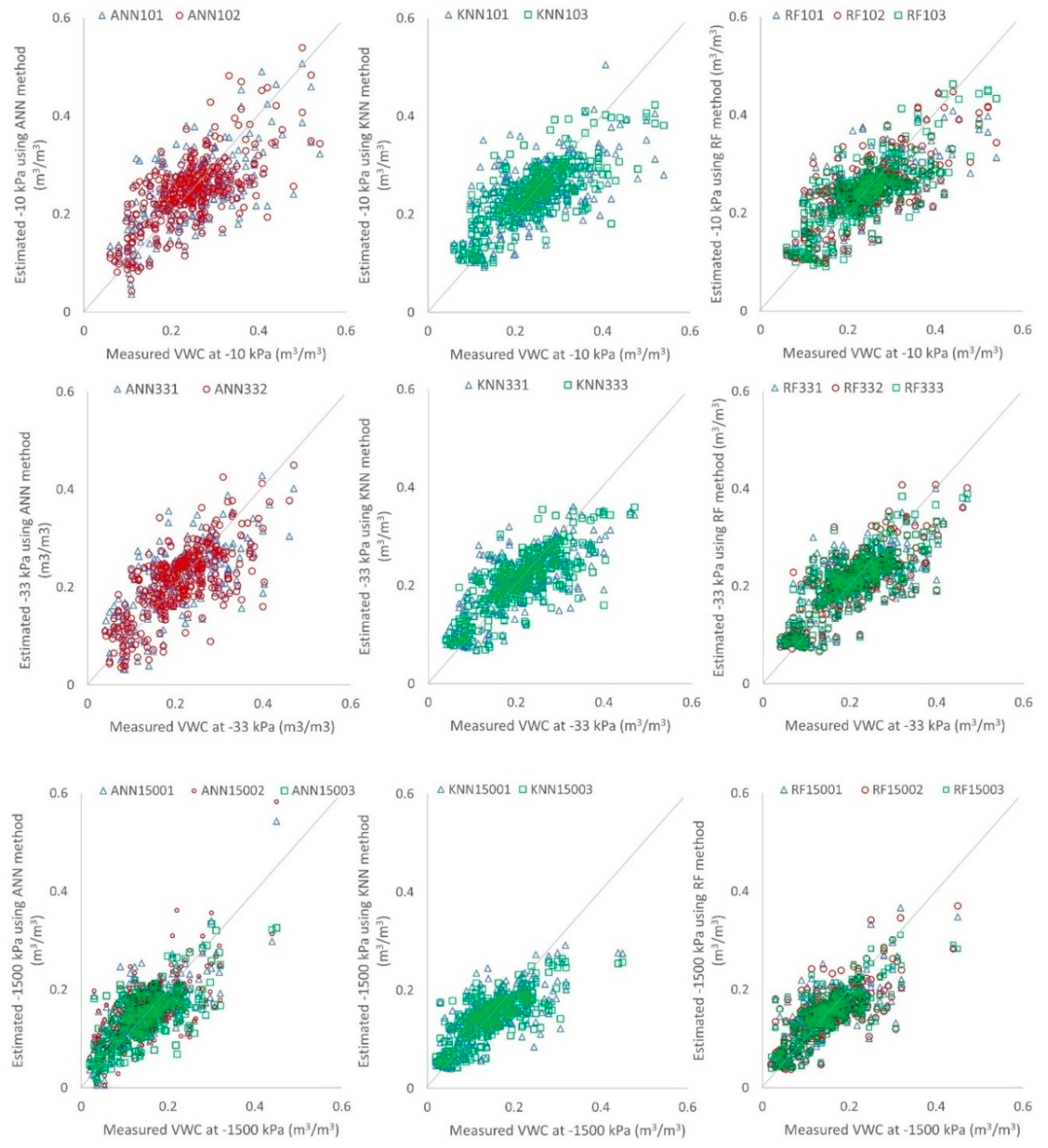
Figure 1 shows the relationships of measured VWC and PTF-estimated VWC for different input levels assessed by different machine learning algorithms. The closeness of points to the 1:1 line indicates the model’s efficiency. Figure 1 shows the superiority of the RF algorithm to the other selected algorithms, with the observations strictly related to the predictions of the PTFs developed by the RF algorithm. Furthermore, it shows accuracy enhancement with the addition of BD and OC as input parameters for the model predictions of the RF algorithm. Figure 1 shows that the linearity of the observed–estimated relationship increases with the decrease in VWCs of soils, as VWC1500 showed the closest and most stable relationship compared to VWC33 and VWC10. A similar relationship was reported by Gunarathna et al. [6] for their PTFs developed using the multiple linear regression approach. With the addition of BD and OC, only the RF algorithm showed improved performances for VWC33 and VWC1500 by the RF method. The KNN algorithm slightly underpredicted both FC and PWP at most input levels, especially in soils with higher FC and PWP. Among the targeted VWCs, VWC10 showed the highest error among the PTFs developed using the KNN algorithm. Among the PTFs developed using the ANN algorithm, those developed to estimate VWC10 and VWC33 showed poor performance compared to those developed to estimate VWC1500.
3.3. Error Distribution of Developed Pedotransfer Functions (PTFs) to Estimate Volumetric Water Content (VWC) of Tropical Sri Lankan Soils at −10, −33, and −1500 kPa
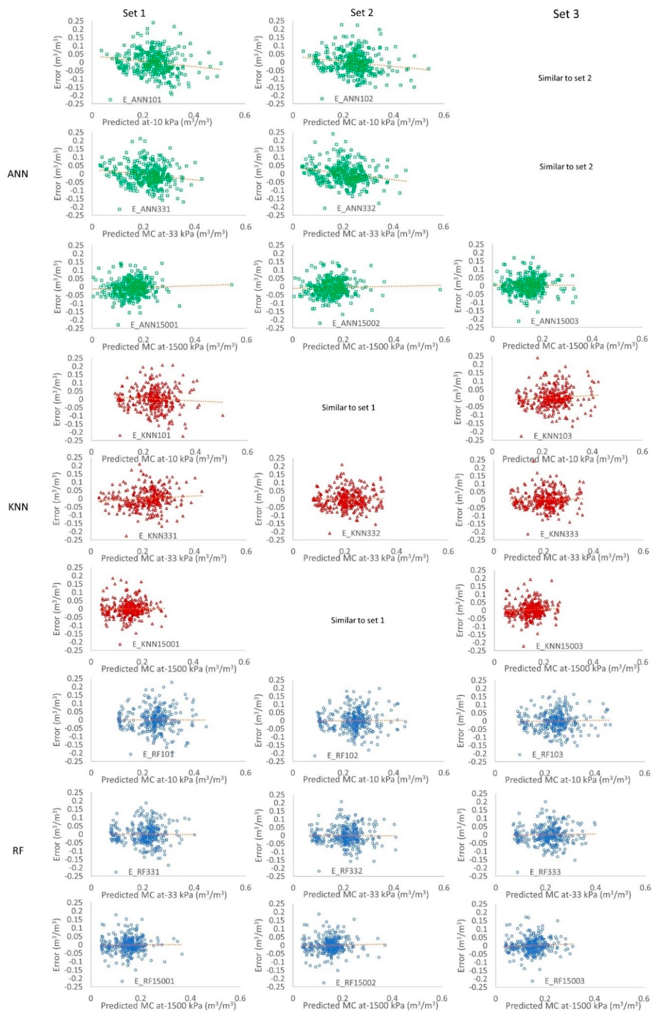
Figure 2 shows the distribution of residuals of PTF predictions. Errors of all PTFs show symmetric distribution, with a tendency to cluster in the middle of the plots. The error is clustered around the 0 (of the Y-axis), without any apparent pattern. Furthermore, the error did not show any trend. Therefore, the residual analysis confirmed the random distribution of error in all three algorithms, input levels, and target VWC levels. Hence, model predictions can be accepted as fair predictions. The RF algorithm showed comparatively better error distribution (fewer scattered data points compared to the central cluster near the 0 of the Y-axis) compared to the other two algorithms. Furthermore, error analysis confirmed that there are no outliers in the dataset, which was also confirmed using the inbuilt function of data preprocessing of WEKA 3.8.
Figure 3 shows the relationship between the percentage of points predicted within the tolerance (Y-axis), with error tolerance on the X-axis. The error on the X-axis is the absolute error. The resulting curve estimates the cumulative distribution function of the error, which is known as the error characteristics curves. The error characteristics curves showed that more than 60% of observations were within the error tolerance of 0.05 m3/m3 for all algorithms for all input levels, except the ANN algorithm, to predict VWC10 using SSC as the input variable (Figure 4). With the addition of BD as an input variable to SSC (Set 2) and the addition of OC to the Set 2 (Set 3), the curves moved upwards, closer to 1, confirming the improved accuracy with the addition of BD and OC. According to the performance shown in Table 4 and Figure 2, Figure 3 and Figure 4, we suggest using input level 3 (SSC, BD, and OC) to estimate VWC 10 and VWC33 (field capacity) with the RF or KNN algorithm for tropical Sri Lankan soils. To estimate the VWC1500 (permanent wilting point), we suggest using the RF algorithm, using SSC, BD, and OC as input methods. However, the use of Set 1, 2, or 3 depends on the availability of data, as most of the available datasets and laboratory facilities are limited to Sri Lanka. For places where data are limited, SSC data can be used to predict field capacity and wilting point with acceptable accuracy by applying the RF algorithm.
Error characteristic curves (Figure 3) show that the PTFs developed by the KNN and RF algorithms can estimate FC with reasonable accuracy. Therefore, field-level assessment of field capacity can successfully be replaced by the PTFs developed using the RF and KNN algorithms. However, attention should be paid to the accuracy requirement of the user. Error characteristic curves (Figure 4) show that the PTFs developed by the RF and KNN algorithms to estimate −1500 kPa were able to estimate over 80% of the population with an error less than 0.05 m3/m3 using any input level. Therefore, the estimation of PWP is quite accurate and can be done even with minimum inputs such as SSC. The estimation of PWP using laborious and resource-consuming field- or laboratory-level experiments can be successfully replaced by the PTFs developed by the RF or KNN algorithms. The PTFs developed by the RF or KNN algorithm using SSC, BD, and OC predicted about 70% of the population within an error range of 0.05 m3/m3. Hence, the PTFs developed by the RF and KNN algorithms can be successfully used to predict field capacity with reasonably good accuracy.
3.4. Comparison of the Pedotransfer Functions (PTFs) Developed by Machine Learning Algorithms with Previously Reported PTFs Using MLR Method
Gunarathna et al. [6] developed PTFs to estimate VWC at −10, −33, and −1500 kPa using different input levels. We calculated the VWC of −10, −33, and −1500 kPa for respective input levels of this study using the equation from Gunarathna et al. [6]. Compared to their results, we found that, regardless of the level of input attributes, the PTFs developed by the ANN algorithm were inferior to those developed by MLR (Figure 4). Fereshte [29] and Minasny et al. [85] also reported the inferiority of ANN in predicting VWC at −10, −33, and −1500 kPa. Except for the cases with low input level (Set 1) and high moisture levels (−10 and −33 kPa), the PTFs developed by the RF algorithm were superior to the results reported by Gunarathna et al. [6] using MLR. The KNN algorithm also showed superior results to those from Gunarathna et al. [6] for high input (Set 3) and high moisture levels. Other researchers have reported that, at high moisture levels, the KNN algorithm was a competitive alternative to MLR for predicting points on the water retention curve [86] and a competitive alternative to the ANN algorithm for predicting the cation exchange capacity [87]. For cases with low moisture levels (−1500 kPa), for all input levels, the results reported by Gunarathna et al. [6] were generally superior to the PTFs developed by the KNN and ANN algorithms, while the RF algorithm showed superior results to MLR. The RF algorithm showed reasonable or good results for all input levels and target VWC levels, except VWC10 with SSC. With high input levels (Set 3), the RF algorithm showed good performance at all target VWC levels.
3.5. Inclusion of Volumetric Water Content as an Input Parameter
We searched for ways to increase the accuracy of PTFs when estimating PWP by further refining them using VWC [71,72]. We used VWC10 as an input along with SSC, BD, and OC to estimate the PWP of tropical Sri Lankan soils. Furthermore, we refined the PTFs to estimate VWC33 using VWC10 as an input variable. VWC10 is easily measurable compared to VWC33 and in most cases VWC33 is considered as FC under Sri Lankan conditions. In the feature selection process of both VWC levels, all three algorithms selected VWC10 as an input. Figure 5 and Table 6 show the accuracy of the new PTFs developed by including VWC10 as an input. The results revealed that the inclusion of VWC10 as an input tremendously increased the performance of all algorithms; however, RF is still the best. According to the error characteristics curves, the PTFs developed by the KNN and RF algorithms (to predict PWP) predicted more than 60% of the population within an error tolerance level of 0.02 m3/m3 and over 90% of the population within an error tolerance level of 0.05 m3/m3. In the case of FC, all the algorithms predicted over 70% and 95% of the population within an error tolerance of 0.02 m3/m3 and 0.05 m3/m3, respectively. All the statistical criteria confirmed the excellent predictability of the PTFs developed by all three algorithms. Few studies tried to use VWCs as inputs of PTFs. However, almost all studies attempted to develop parametric PTFs [71,72,88,89]. In those studies, they used VWC33 and VWC1500 as input(s) of the PTFs developed to estimate soil water retention parameters or saturated hydraulic conductivity. With the inclusion of VWCs as inputs, they reported improvements in their PTFs. The ROSETTA model is a famous example of using VWCs as input parameters to estimate water retention parameters [72]. In our study, we noticed an improvement in the performance of PTFs with the inclusion of VWC10 as an input parameter. Since the estimation of VWC10 is much easier than that of PWP and also significantly easier than the FC (in most studies in Sri Lanka used VWC33 as FC), the inclusion of VWC10 as an input parameter could be an excellent option to increase the accuracy of PTFs.
3.6. Functionality of Volumetric Water Content (VWC)-Supported Pedotransfer Functions (PTFs)
We estimated the available water content (AWC) of tropical Sri Lankan soils using field-observed FC and PWP and PTF-estimated FC and PWP to check the functionality of the developed PTFs (Figure 6). The results showed that AWCs calculated using PTFs have quite a close relationship with the measurement-based AWC values. Among the three machine learning algorithms, RF showed a better correlation compared to the other two algorithms because of the comparatively better predictions of both FC and PWP. Residual plots (Figure 7) show that both FC and PWP reported the random distribution of errors compared to the AWC. Error shows a slight negative trend, which indicates a slight overestimation of AWC, especially for soils with a high water-holding capacity. Gunarathna et al. [6] reported similarities of observations and PTF estimations in irrigation water estimations for the tropical Sri Lankan soils. The PTFs developed here show significantly better estimations of FC and PWP of tropical Sri Lankan soils than Gunarathna et al. [6] presented. Hence, this overestimation may not be an issue for field-level applications. However, the authors suggested more studies to further finetune the available PTFs or develop new PTFs for tropical Sri Lankan soils. Furthermore, we suggest further functionality assessments of these PTFs for numerous uses, including process-based models.
4. Conclusions
We used a wrapper approach and a best-first search method to identify ideal candidates for developing PTFs using different machine learning algorithms. Different machine learning algorithms choose different input combinations to develop PTFs for targeted VWCs. We developed PTFs to estimate the VWC of Sri Lankan soils at −10 (VWC10), −33 (VWC33), and −1500 (VWC1500) kPa with good accuracy using different machine learning algorithms (ANN, KNN, and RF) with different input levels for SSC (Set 1), SSC + BD (Set 2), and SSC + BD + OC (Set 3). Statistical criteria, residual analysis, and error characteristic curves were used to compare the performance of machine learning algorithms. We found that the RF algorithm gives significantly better results compared to the other selected machine learning algorithms for all input levels and targeted VWC levels. Among the input combinations, a combination of SSC, BD, and OC led to significantly better performance compared to the other input levels. We compared our PTFs with the PTFs reported by Gunarathna et al. [6] for tropical Sri Lankan soils. We found that the PTFs developed by the RF algorithm are superior to those reported previously, especially with high input attributes. We assessed the possibility of using VWC10 to develop PTFs to estimate VWC33 and VWC1500 using machine learning algorithms. With that addition, all three machine learning algorithms boosted the performance and showed superior accuracy compared to the PTFs developed earlier. Among the three machine learning algorithms, RF was the best. We studied the functionality of VWC10-supported PTFs to estimate the AWC of tropical soils and found that those PTFs were reliable for estimating the AWC of tropical Sri Lankan soils.
We developed a hierarchy of PTFs for input ranges using different machine learning algorithms and identified the RF algorithm as the most robust machine learning algorithm for developing PTFs for tropical Sri Lankan soils. Therefore, we recommend that the PTFs developed using the RF algorithm be incorporated in the relevant software to make up for the data gaps in tropical regions. Since SSC alone can estimate FC and PWP with reasonable accuracy, we suggest using a set of options (based on input level) to giving users the ability to choose input combinations (such as SSC, SSC and BD, SSC, BD, and OC and SSC, BD, OC, and VWC10). This may help with catering to most users in data-scarce tropical regions. Although the new PTFs had good accuracy for AWC estimations, we suggest further validation of the functionality of these PTFs for numerous applications, including process-based models.
Author Contributions
M.H.J.P.G. and K.S. conceptualized, conceived and performed, and K.S., T.N. and K.M. supervised the study. M.H.J.P.G., M.K.N.K. and K.S. interpreted data and developed the manuscript. All authors read and approved the final manuscript.
Funding
This research received no external funding.
Acknowledgments
We acknowledge all the authors of the original data source, Fact sheets of Benchmark Soils of the Dry Zone of Sri Lanka, SRICANSOL Project of the Soil Science Society of Sri Lanka, for developing this useful database and letting scientists to use it for research.
Conflicts of Interest
The authors declare no conflict of interest.
References
- Patil, N.G.; Singh, S.K. Pedotransfer Functions for Estimating Soil Hydraulic Properties: A Review. Pedosphere 2016, 26, 417–430. [Google Scholar] [CrossRef]
- Minasny, B.; Hartemink, A.E. Predicting soil properties in the tropics. Earth-Sci. Rev. 2011, 106, 52–62. [Google Scholar] [CrossRef]
- Rustanto, A.; Booij, M.J.; Wösten, H.; Hoekstra, A.Y. Application and recalibration of soil water retention pedotransfer functions in a tropical upstream catchment: Case study in Bengawan Solo, Indonesia. J. Hydrol. Hydromech. 2017, 65, 307–320. [Google Scholar] [CrossRef]
- Tomasella, J.; Hodnett, M. Pedotransfer functions for tropical soils. In Synchrotron-Based Techniques in Soils and Sediments; Elsevier B.V.: Amsterdam, The Netherlands, 2004; Volume 30, pp. 415–429. [Google Scholar]
- Bouma, J. Using Soil Survey Data for Quantitative Land Evaluation. Adv. Soil Sci. 1989, 9, 177–213. [Google Scholar]
- Gunarathna, M.; Sakai, K.; Nakandakari, T.; Momii, K.; Kumari, M.; Amarasekara, M. Pedotransfer functions to estimate hydraulic properties of tropical Sri Lankan soils. Soil Tillage Res. 2019, 190, 109–119. [Google Scholar] [CrossRef]
- Botula, Y.-D.; Van Ranst, E.; Cornelis, W.M. Pedotransfer functions to predict water retention for soils of the humid tropics: A review. Rev. Bras. Ciênc. Solo 2014, 38, 679–698. [Google Scholar] [CrossRef]
- Nguyen, P.M.; De Pue, J.; Van Le, K.; Cornelis, W. Impact of regression methods on improved effects of soil structure on soil water retention estimates. J. Hydrol. 2015, 525, 598–606. [Google Scholar] [CrossRef]
- Adhikary, P.P.; Chakraborty, D.; Kalra, N.; Sachdev, C.B.; Patra, A.K.; Kumar, S.; Tomar, R.K.; Chandna, P.; Raghav, D.; Agrawal, K.; et al. Pedotransfer functions for predicting the hydraulic properties of Indian soils. Soil Res. 2008, 46, 476–484. [Google Scholar] [CrossRef]
- Botula, Y. Indirect Methods to Predict Hydrophysical Properties of Soils of Lower Congo; Ghent University: Ghent, Belgium, 2013. [Google Scholar]
- Mdemu, M.V. Evaluation and Development of Pedotransfer Functions for Estimating Soil Water Holding Capacity in the Tropics: The Case of Sokoine University of Agriculture Farm in Morogoro, Tanzania. J. Geogr. Geol. 2015, 7, 1–9. [Google Scholar] [CrossRef]
- Mihalikova, M.; Matula, S.; Dolezal, F. Application of k-nearest code for the improvement of class pedotransfer functions and countrywide field capacity and wilting point maps. Soil Water Res. 2014, 9, 1–8. [Google Scholar] [CrossRef]
- Nemes, A.; Schaap, M.G.; Wösten, J.H.M. Functional Evaluation of Pedotransfer Functions Derived from Different Scales of Data Collection. Soil Sci. Soc. Am. J. 2003, 67, 1093. [Google Scholar] [CrossRef]
- Jana, R.B.; Mohanty, B.P. Enhancing PTFs with remotely sensed data for multi-scale soil water retention estimation. J. Hydrol. 2011, 399, 201–211. [Google Scholar] [CrossRef]
- D’Emilio, A.; Aiello, R.; Consoli, S.; Vanella, D.; Iovino, M. Artificial Neural Networks for Predicting the Water Retention Curve of Sicilian Agricultural Soils. Water 2018, 10, 1431. [Google Scholar] [CrossRef]
- Rodríguez-Lado, L.; Rial, M.; Taboada, T.; Cortizas, A.M. A Pedotransfer Function to Map Soil Bulk Density from Limited Data. Procedia Environ. Sci. 2015, 27, 45–48. [Google Scholar] [CrossRef] [Green Version]
- De Souza, E.; Filho, E.I.F.; Batjes, N.H.; Dos Santos, G.R.; Pontes, L.M.; Schaefer, C.E.G.R. Pedotransfer functions to estimate bulk density from soil properties and environmental covariates: Rio Doce basin. Sci. Agric. 2016, 73, 525–534. [Google Scholar] [CrossRef] [Green Version]
- Tayfur, G.; Singh, V.P.; Moramarco, T.; Barbetta, S. Flood Hydrograph Prediction Using Machine Learning Methods. Water 2018, 10, 968. [Google Scholar] [CrossRef]
- Saadi, M.; Oudin, L.; Ribstein, P. Random Forest Ability in Regionalizing Hourly Hydrological Model Parameters. Water 2019, 11, 1540. [Google Scholar] [CrossRef]
- Diez-Sierra, J.; Del Jesus, M. Subdaily Rainfall Estimation through Daily Rainfall Downscaling Using Random Forests in Spain. Water 2019, 11, 125. [Google Scholar] [CrossRef]
- Alizadeh, Z.; Yazdi, J.; Kim, J.H.; Al-Shamiri, A.K. Assessment of Machine Learning Techniques for Monthly Flow Prediction. Water 2018, 10, 1676. [Google Scholar] [CrossRef]
- Chang, L.-C.; Chang, F.-J.; Yang, S.-N.; Kao, I.-F.; Ku, Y.-Y.; Kuo, C.-L.; Amin, I.M.Z.B.M. Building an Intelligent Hydroinformatics Integration Platform for Regional Flood Inundation Warning Systems. Water 2018, 11, 9. [Google Scholar] [CrossRef]
- Hu, C.; Wu, Q.; Li, H.; Jian, S.; Li, N.; Lou, Z. Deep Learning with a Long Short-Term Memory Networks Approach for Rainfall-Runoff Simulation. Water 2018, 10, 1543. [Google Scholar] [CrossRef]
- Mosavi, A.; Ozturk, P.; Chau, K.-W. Flood Prediction Using Machine Learning Models: Literature Review. Water 2018, 10, 1536. [Google Scholar] [CrossRef]
- Chang, L.-C.; Amin, M.Z.M.; Yang, S.-N.; Chang, F.-J. Building ANN-Based Regional Multi-Step-Ahead Flood Inundation Forecast Models. Water 2018, 10, 1283. [Google Scholar] [CrossRef]
- Hastie, T.; Tibshirani, R.; Friedman, J. The Elements of Statistical Learning, 2nd ed.; Springer: New York, NY, USA, 2009; ISBN 978-0-387-84857-0. [Google Scholar]
- Wang, G.; Zhanga, Y.; Yu, N. Prediction of Soil Water Retention and Available Water of Sandy Soils using Pedotransfer Functions. Procedia Eng. 2012, 37, 49–53. [Google Scholar] [CrossRef] [Green Version]
- Merdun, H. Alternative methods in the development of pedotransfer functions for soil hydraulic characteristics. Eurasian Soil Sci. 2010, 43, 62–71. [Google Scholar] [CrossRef]
- Fereshte, H.F. Evaluation of Artificial Neural Network and Regression PTFS in Estimating Some Soil Hydraulic Parameters. ProEnvironment 2014, 7, 10–20. [Google Scholar]
- Sanchez, P.A. Linking climate change research with food security and poverty reduction in the tropics. Agric. Ecosyst. Environ. 2000, 82, 371–383. [Google Scholar] [CrossRef]
- Porter, J.R.; Xie, L.; Challinor, A.J.; Cochrane, K.; Howden, S.M.; Iqbal, M.M.; Lobell, D.B.; Travasso, M.I. Food Security and Food Production Systems. In Climate Change 2014: Impacts, Adaptation, and Vulnerability. Part A: Global and Sectoral Aspects. Contribution of Working Group II to the Fifth Assessment Report of the Intergovernmental Panel on Climate Change; Field, C.B., Barros, V.R., Dokken, D.J., Mach, K.J., Mastrandrea, M.D., Bilir, T.E., Chatterjee, M., Ebi, K.L., Estrada, Y.O., Genova, R.C., Eds.; Cambridge University Press: Cambridge, UK; New York, NY, USA, 2014; pp. 485–533. ISBN 9781107641655. [Google Scholar]
- Tito, R.; Vasconcelos, H.L.; Feeley, K.J. Global climate change increases risk of crop yield losses and food insecurity in the tropical Andes. Glob. Chang. Boil. 2017, 24, e592–e602. [Google Scholar] [CrossRef]
- Kang, Y.; Khan, S.; Ma, X. Climate change impacts on crop yield, crop water productivity and food security—A review. Prog. Nat. Sci. 2009, 19, 1665–1674. [Google Scholar] [CrossRef]
- Gaydon, D.S.; Balwinder-Singh; Wang, E.; Poulton, P.L.; Ahmad, B.; Ahmed, F.; Akhter, S.; Ali, I.; Amarasingha, R.; Chaki, A.K.; et al. Evaluation of the APSIM model in cropping systems of Asia. Field Crops Res. 2017, 204, 52–75. [Google Scholar] [CrossRef]
- Zubair, L.; Nissanka, S.P.; Weerakoon, W.M.W.; Herath, D.I.; Karunaratne, A.S.; Agalawatte, P.; Herath, R.M.; Yahiya, S.Z.; Punyawardhene, B.V.R.; Vishwanathan, J.; et al. Climate Change Impacts on Rice Farming Systems in Northwestern Sri Lanka. In Handbook of Climate Change and Agroecosystems; Imperial College Press: London, UK, 2015; pp. 315–352. [Google Scholar] [Green Version]
- Vanuytrecht, E.; Raes, D.; Steduto, P.; Hsiao, T.C.; Fereres, E.; Heng, L.K.; Vila, M.G.; Moreno, P.M. AquaCrop: FAO’s crop water productivity and yield response model. Environ. Model. Softw. 2014, 62, 351–360. [Google Scholar] [CrossRef]
- Gassman, P.W.; Reyes, M.R.; Green, C.H.; Arnold, J.G. The Soil and Water Assessment Tool: Historical Development, Applications, and Future Research Directions. Trans. ASABE 2007, 50, 1211–1250. [Google Scholar] [CrossRef] [Green Version]
- Jones, J.W.; Tsuji, G.Y.; Hoogenboom, G.; Hunt, L.A.; Thornton, P.K.; Wilkens, P.W.; Imamura, D.T.; Bowen, W.T.; Singh, U.; Vries, F.W.T.P. Decision support system for agrotechnology transfer: DSSAT v3. In Understanding Options for Agricultural Production; Springer Science and Business Media: Berlin, Germany, 1998; Volume 7, pp. 157–177. [Google Scholar]
- Keating, B.; Carberry, P.; Hammer, G.; Probert, M.; Robertson, M.; Holzworth, D.; Huth, N.; Hargreaves, J.; Meinke, H.; Hochman, Z.; et al. An overview of APSIM, a model designed for farming systems simulation. Eur. J. Agron. 2003, 18, 267–288. [Google Scholar] [CrossRef] [Green Version]
- Gunarathna, M.; Sakai, K.; Nakandakari, T.; Momii, K.; Kumari, M. Sensitivity Analysis of Plant- and Cultivar-Specific Parameters of APSIM-Sugar Model: Variation between Climates and Management Conditions. Agronomy 2019, 9, 242. [Google Scholar] [CrossRef]
- Gunarathna, M.H.J.P.; Sakai, K.; Kumari, M.K.N. Can crop modeling sucess with estimated soil hydraulic parameters? In Proceedings of the PAWEES-INWEPF International Conference Nara 2018, Nara, Japan, 9–17 May 2018; pp. 461–470. [Google Scholar]
- Gunarathna, M.H.J.P.; Sakai, K. Evaluation of pedotransfer functions for estimating soil moisture constants: A study on soils in dry zone of tropical Sri Lanka. Int. J. Adv. Sci. Eng. Technol. 2018, 6, 15–19. [Google Scholar]
- Senarath, A.; Dassanayake, A.R.; Mapa, R.B. Bench Mark Soils of the Wet Zone: Factsheets; Mapa, R.B., Somasiri, S., Nagarajah, S.L., Eds.; Soil Science Society of Sri Lanka: Kandy, Sri Lanka, 1999. [Google Scholar]
- Dassanayake, A.R.; Somasiri, L.L.W.; Mapa, R.B. Benchmark Soils of the Intermediate Zone: Factsheets; Mapa, R.B., Dassanayake, A.R., Nayakekorale, H.B., Eds.; Soil Science Society of Sri Lanka: Kandy, Sri Lanka, 2005. [Google Scholar]
- Dassanayake, A.R.; De Silva, G.G.R.; Mapa, R.B.; Kumaragamage, D. Benchmark Soils of the Dry Zone of Sri Lanka: Factsheets; Mapa, R.B., Somasiri, S., Dassanayake, A.R., Eds.; Soil Science Society of Sri Lanka: Kandy, Sri Lanka, 2010. [Google Scholar]
- Frank, E.; Holmes, G.; Pfahringer, B.; Reutemann, P.; Witten, I.H.; Hall, M. The WEKA data mining software: An update. ACM SIGKDD Explor. Newsl. 2009, 11, 10. [Google Scholar]
- Frank, E.; Hall, M.A.; Witten, I.H. The WEKA Workbench. In Data Mining: Practical Machine Learning Tools and Techniques, 4th ed.; Morgan Kaufmann: Burlington, MA, USA, 2016. [Google Scholar]
- Pachepsky, Y.; Schaap, M. Data mining and exploration techniques. In Synchrotron-Based Techniques in Soils and Sediments; Elsevier B.V.: Amsterdam, The Netherlands, 2004; Volume 30, pp. 21–32. [Google Scholar]
- Kohavi, R.; John, G.H. Wrappers for feature subset selection. Artif. Intell. 1997, 97, 273–324. [Google Scholar] [CrossRef] [Green Version]
- Hall, M.; Holmes, G. Benchmarking attribute selection techniques for discrete class data mining. IEEE Trans. Knowl. Data Eng. 2003, 15, 1437–1447. [Google Scholar] [CrossRef]
- Russel, S.J.; Norvig, P. Artificial Intelligence—A modern Approach, 3rd ed.; Pearson Education, Inc.: Upper Saddle River, NJ, USA, 2010; ISBN 9780136042594. [Google Scholar]
- Dechter, R.; Pearl, J. Generalized best-first search strategies and the optimality af A. J. ACM 1985, 32, 505–536. [Google Scholar] [CrossRef]
- Liu, H.; Setiono, R. Feature selection via discretization. IEEE Trans. Knowl. Data Eng. 1997, 9, 642–645. [Google Scholar]
- Gheyas, I.A.; Smith, L.S. Feature subset selection in large dimensionality domains. Pattern Recognit. 2010, 43, 5–13. [Google Scholar] [CrossRef] [Green Version]
- Araya, S.N.; Ghezzehei, T.A. Using Machine Learning for Prediction of Saturated Hydraulic Conductivity and Its Sensitivity to Soil Structural Perturbations. Water Resour. Res. 2019, 55, 5715–5737. [Google Scholar] [CrossRef]
- Cover, T.; Hart, P. Nearest neighbor pattern classification. IEEE Trans. Inf. Theory 1967, 13, 21–27. [Google Scholar] [CrossRef]
- Nemes, A.; Rawls, W.J.; Pachepsky, Y.A. Use of the Nonparametric Nearest Neighbor Approach to Estimate Soil Hydraulic Properties. Soil Sci. Soc. Am. J. 2006, 70, 327–336. [Google Scholar] [CrossRef]
- Hart, P.E. The condensed nearest neighbor rule. IEEE Trans. Inf. Theory 1968, 14, 515–516. [Google Scholar] [CrossRef]
- Aha, D.W.; Kibler, D.; Albert, M.K. Instance-Based Learning Algorithms. Mach. Learn. 1991, 6, 37–66. [Google Scholar] [CrossRef]
- De Sá, A.G.C.; Freitas, A.A.; Pappa, G.L. Multi-label classification search space in the MEKA software. arXiv 2018, arXiv:1811.11353. [Google Scholar]
- Haykin, S. Neural Networks—A Comprehensive Foundation, 2nd ed.; Pearson Education (Singapore) Pte. Ltd.: Delhi, India, 2005. [Google Scholar]
- Van Looy, K.; Bouma, J.; Herbst, M.; Koestel, J.; Minasny, B.; Mishra, U.; Montzka, C.; Nemes, A.; Pachepsky, Y.A.; Padarian, J.; et al. Pedotransfer Functions in Earth System Science: Challenges and Perspectives. Rev. Geophys. 2017, 55, 1199–1256. [Google Scholar] [CrossRef] [Green Version]
- Zhou, J.; Peng, T.; Zhang, C.; Sun, N. Data Pre-Analysis and Ensemble of Various Artificial Neural Networks for Monthly Streamflow Forecasting. Water 2018, 10, 628. [Google Scholar] [CrossRef]
- Jabbari, A.; Bae, D.-H. Application of Artificial Neural Networks for Accuracy Enhancements of Real-Time Flood Forecasting in the Imjin Basin. Water 2018, 10, 1626. [Google Scholar] [CrossRef]
- Goodfellow, I.; Bengio, Y.; Courville, A. Deep Learning; MIT Press: Cambridge, MA, USA, 2016. [Google Scholar]
- Bengio, Y. Practical Recommendations for Gradient-Based Training of Deep Architectures. In Computer Vision—ECCV 2012; Springer Science and Business Media: Berlin, Germany, 2012; Volume 7700, pp. 437–478. [Google Scholar]
- Sheela, K.G.; Deepa, S.N. Review on Methods to Fix Number of Hidden Neurons in Neural Networks. Math. Probl. Eng. 2013, 2013, 1–11. [Google Scholar] [CrossRef] [Green Version]
- Breiman, L. Random forests. Mach. Learn. 2001, 45, 5–32. [Google Scholar] [CrossRef]
- Han, J.; Kamber, M.; Pei, J. Data Mining: Concepts and Techniques; Elsevier: Amsterdam, The Netherlands, 2012; ISBN 978-0-12-381479-1. [Google Scholar]
- Liaw, A.; Wiener, M. Classification and Regression by randomForest. R News 2002, 2, 18–22. [Google Scholar] [CrossRef]
- Zhang, Y.; Schaap, M.G. Weighted recalibration of the Rosetta pedotransfer model with improved estimates of hydraulic parameter distributions and summary statistics (Rosetta3). J. Hydrol. 2017, 547, 39–53. [Google Scholar] [CrossRef] [Green Version]
- Schaap, M.G.; Leij, F.J.; Genuchten, M.T. Van rosetta: A computer program for estimating soil hydraulic parameters with hierarchical pedotransfer functions. J. Hydrol. 2001, 251, 163–176. [Google Scholar] [CrossRef]
- Zambrano-Bigiarini, M. Package ‘hydroGOF: Goodness-of-Fit Functions for Comparison of Simulated and Observed Hydrological Time Series’; R Package Version 0.3-10. Available online: http://hzambran.github.io/hydroGOF/ (accessed on 15 January 2019).
- R Core Team. R: A Language and Environment for Statistical Computing; R Foundation for Statistical Computing: Vienna, Austria; Available online: https://www.R-project.org/2018 (accessed on 15 January 2019).
- Schaap, M. Accuracy and uncertainty in PTF predictions. In Synchrotron-Based Techniques in Soils and Sediments; Elsevier B.V.: Amsterdam, The Netherlands, 2004; Volume 30, pp. 33–43. [Google Scholar]
- Nash, J.; Sutcliffe, J. River flow forecasting through conceptual models part I—A discussion of principles. J. Hydrol. 1970, 10, 282–290. [Google Scholar] [CrossRef]
- Willmott, C.J. ON THE VALIDATION OF MODELS. Phys. Geogr. 1981, 2, 184–194. [Google Scholar] [CrossRef]
- Camargo, A.P.; Sentelhas, P.C. Performance evaluation of different potential evapotranspiration estimation methods in the state of Sao Paulo, Brazil. Rev. Bras. Agrometeorol. 1997, 5, 89–97. [Google Scholar] [CrossRef]
- Monteiro, L.A.; Sentelhas, P.C. Calibration and testing of an agrometeorological model for the estimation of soybean yields in different Brazilian regions. Acta Sci. Agron. 2014, 36, 265. [Google Scholar] [CrossRef] [Green Version]
- Diebold, F.X.; Mariano, R.S. Comparing predictive accuracy. J. Bus. Econ. Stat. 1995, 13, 253–263. [Google Scholar]
- Hyndman, R.J.; Khandakar, Y. Automatic Time Series Forecasting: The forecast Package for R. J. Stat. Softw. 2008, 27, 1–22. [Google Scholar] [CrossRef]
- Hyndman, R.J.; Athanasopoulos, G.; Bergmeir, C.; Caceres, G.; Chhay, L.; O’Hara-Wild, M.; Petropoulos, F.; Razbash, S.; Wang, E.; Yasmeen, F. Forecast: Forecasting Functions for Time Series and Linear Models. R Package Version 8.7. Available online: http://pkg.robjhyndman.com/forecast/2019 (accessed on 15 March 2019).
- Berg, M.V.D.; Klamt, E.; Van Reeuwijk, L.; Sombroek, W. Pedotransfer functions for the estimation of moisture retention characteristics of Ferralsols and related soils. Geoderma 1997, 78, 161–180. [Google Scholar] [CrossRef]
- Gaiser, T.; Graef, F.; Cordeiro, J.C. Water retention characteristics of soils with contrasting clay mineral composition in semi-arid tropical regions. Soil Res. 2000, 38, 523–536. [Google Scholar] [CrossRef]
- Minasny, B.; McBratney, A.B.; Bristow, K.L. Comparison of different approaches to the development of pedotransfer functions for water-retention curves. Geoderma 1999, 93, 225–253. [Google Scholar] [CrossRef]
- Botula, Y.-D.; Nemes, A.; Mafuka, P.; Van Ranst, E.; Cornelis, W.M. Prediction of Water Retention of Soils from the Humid Tropics by the Nonparametric—Nearest Neighbor Approach. Vadose Zone J. 2013, 12, 12. [Google Scholar] [CrossRef]
- Zolfaghari, A.; Taghizadeh-Mehrjardi, R.; Moshki, A.; Malone, B.; Weldeyohannes, A.; Sarmadian, F.; Yazdani, M.; Malone, B. Using the nonparametric k-nearest neighbor approach for predicting cation exchange capacity. Geoderma 2016, 265, 111–119. [Google Scholar] [CrossRef]
- Ahuja, L.R.; Naney, J.W.; Williams, R.D. Estimating Soil Water Characteristics from Simpler Properties or Limited Data. Soil Sci. Soc. Am. J. 2010, 49, 1100. [Google Scholar] [CrossRef]
- Paydar, Z.; Cresswell, H.P. Water retention in Australian soils. II. Prediction using particle size, bulk density, and other properties. Aust. J. Soil Res. 1996, 34, 679–693. [Google Scholar] [CrossRef]
Figure 1.
Relationship between measured and estimated volumetric water contents under different machine learning methods.
Figure 1.
Relationship between measured and estimated volumetric water contents under different machine learning methods.

Figure 2.
Residual plots of different input levels, target levels, and different algorithms.

Figure 3.
Variation of cumulative accuracy on pedotransfer functions (PTF) development methods and input levels.
Figure 3.
Variation of cumulative accuracy on pedotransfer functions (PTF) development methods and input levels.

Figure 4.
Comparison of confidence indices of the pedotransfer functions (PTFs) developed using machine learning algorithms in this study and results reported by Gunarathna et al. [6] for the multiple linear regression (MLR) method.
Figure 4.
Comparison of confidence indices of the pedotransfer functions (PTFs) developed using machine learning algorithms in this study and results reported by Gunarathna et al. [6] for the multiple linear regression (MLR) method.

Figure 5.
Performance of volumetric water content (VWC)10-supported pedotransfer functions (PTFs) to estimate VWC33 and VWC1500 of tropical Sri Lankan soils.
Figure 5.
Performance of volumetric water content (VWC)10-supported pedotransfer functions (PTFs) to estimate VWC33 and VWC1500 of tropical Sri Lankan soils.

Figure 6.
Relationship between measurement-based and pedotransfer function (PTF)-based available water content of tropical Sri Lankan soils.
Figure 6.
Relationship between measurement-based and pedotransfer function (PTF)-based available water content of tropical Sri Lankan soils.

Figure 7.
Residuals of field capacity (FC), permanent wilting point (PWP), and available water content (AWC) estimations using different machine learning algorithms.
Figure 7.
Residuals of field capacity (FC), permanent wilting point (PWP), and available water content (AWC) estimations using different machine learning algorithms.


Table 1.
Summary statistics of selected tropical Sri Lankan soils.
| Minimum | Maximum | Mean | SD | Skewness | Kurtosis | CV% | |
|---|---|---|---|---|---|---|---|
| SA (%) | 5.2 | 99.0 | 65.1 | 17.4 | −0.329 | −0.158 | 26.8 |
| SI (%) | 0.0 | 38.6 | 13.1 | 7.7 | 0.703 | 0.503 | 58.8 |
| CL (%) | 1.0 | 61.4 | 21.9 | 13.2 | 0.517 | −0.357 | 60.4 |
| BD (g/cm3) | 1.00 | 2.00 | 1.49 | 0.17 | −0.346 | 0.162 | 11.3 |
| OC (%) | 0.0 | 4.5 | 0.6 | 0.6 | 2.074 | 6.980 | 96.5 |
| VWC10 | 0.06 | 0.54 | 0.24 | 0.09 | 0.434 | 0.419 | 36.9 |
| VWC33 | 0.04 | 0.47 | 0.21 | 0.08 | 0.251 | −0.143 | 39.9 |
| VWC1500 | 0.02 | 0.45 | 0.15 | 0.07 | 0.670 | 1.277 | 46.5 |
SA—Sand; SI—Silt; CL—Clay; BD—Bulk density; OC—Organic carbon; VWCx—Volumetric water content at −10, −33, and −1500 kPa; SD—Standard deviation; CV—Coefficient of variation.
Table 2.
Pearson’s correlation matrix between selected attributes.
| Variable | Sand | Silt | Clay | BD | OC | VWC10 | VWC33 | VWC1500 |
|---|---|---|---|---|---|---|---|---|
| Sand | 1 | |||||||
| Silt | −0.7020 | 1 | ||||||
| Clay | −0.9103 | 0.34429 | 1 | |||||
| BD | 0.42982 | −0.4119 | −0.3274 | 1 | ||||
| OC | −0.1806 | 0.2521 | 0.09184 | −0.3316 | 1 | |||
| VWC10 | −0.7106 | 0.60833 | 0.58319 | −0.3800 | 0.21464 | 1 | ||
| VWC33 | −0.7278 | 0.60326 | 0.60888 | −0.3951 | 0.21325 | 0.96621 | 1 | |
| VWC1500 | −0.7482 | 0.58033 | 0.64906 | −0.404 | 0.28858 | 0.91183 | 0.92891 | 1 |
BD—Bulk density; OC—Organic carbon; VWCx—Volumetric water content at −10, −33, and −1500 kPa.
Table 3.
Attributes selected by each algorithm for each input levels to estimate volumetric water content (VWC) for Sri Lankan soils.
Table 3.
Attributes selected by each algorithm for each input levels to estimate volumetric water content (VWC) for Sri Lankan soils.
| Input Level | VWC | ANN | KNN | RF | ||||||||||||
|---|---|---|---|---|---|---|---|---|---|---|---|---|---|---|---|---|
| SA | SI | CL | BD | OC | SA | SI | CL | BD | OC | SA | SI | CL | BD | OC | ||
| Set 1 | VWC10 | ● | ● | ● | ● | ● | ||||||||||
| VWC33 | ● | ● | ● | ● | ● | |||||||||||
| VWC1500 | ● | ● | ● | ● | ● | |||||||||||
| Set 2 | VWC10 | ● | ● | ● | ● | ● | ● | ● | ||||||||
| VWC33 | ● | ● | ● | ● | ● | ● | ● | ● | ||||||||
| VWC1500 | ● | ● | ● | ● | ● | ● | ● | |||||||||
| Set 3 | VWC10 | ● | ● | ● | ● | ● | ● | ● | ● | ● | ● | ● | ||||
| VWC33 | ● | ● | ● | ● | ● | ● | ● | ● | ● | ● | ● | |||||
| VWC1500 | ● | ● | ● | ● | ● | ● | ● | ● | ● | ● | ||||||
KNN—k-nearest neighbor method; ANN—artificial neural networks; RF—random forest.
Table 4.
Performance of the pedotransfer functions (PTFs) developed to estimate volumetric water content (VWC) by selected algorithms for Sri Lankan soils.
Table 4.
Performance of the pedotransfer functions (PTFs) developed to estimate volumetric water content (VWC) by selected algorithms for Sri Lankan soils.
| Set | Method | r | MAE | RMSE | R2 | d | NSE | CI | DM |
|---|---|---|---|---|---|---|---|---|---|
| VWC10 | |||||||||
| 1 | ANN(3) | 0.665 | 0.0532 | 0.0678 | 0.442 | 0.802 | 0.425 | 0.53 | S |
| KNN(11) | 0.665 | 0.0492 | 0.0669 | 0.442 | 0.789 | 0.438 | 0.52 | S | |
| RF(3) | 0.708 | 0.0467 | 0.0631 | 0.502 | 0.812 | 0.502 | 0.57 | - | |
| 2 | ANN(5) | 0.700 | 0.0507 | 0.0648 | 0.490 | 0.824 | 0.475 | 0.58 | S |
| KNN(11) | 0.665 | 0.0492 | 0.0669 | 0.442 | 0.789 | 0.438 | 0.52 | S | |
| RF(5) | 0.732 | 0.0458 | 0.0608 | 0.539 | 0.830 | 0.538 | 0.61 | - | |
| 3 | ANN(3) | 0.700 | 0.0507 | 0.0648 | 0.490 | 0.824 | 0.475 | 0.58 | S |
| KNN(11) | 0.762 | 0.0420 | 0.0581 | 0.580 | 0.843 | 0.577 | 0.64 | NS | |
| RF(7) | 0.764 | 0.0440 | 0.0577 | 0.583 | 0.851 | 0.583 | 0.65 | - | |
| VWC33 | |||||||||
| 1 | ANN(2) | 0.694 | 0.0479 | 0.0614 | 0.478 | 0.820 | 0.455 | 0.57 | S |
| KNN(12) | 0.708 | 0.0446 | 0.0588 | 0.502 | 0.819 | 0.501 | 0.58 | NS | |
| RF(4) | 0.727 | 0.0435 | 0.0572 | 0.529 | 0.829 | 0.529 | 0.60 | - | |
| 2 | ANN(5) | 0.705 | 0.0467 | 0.0605 | 0.497 | 0.833 | 0.473 | 0.59 | S |
| KNN(12) | 0.754 | 0.0425 | 0.0548 | 0.568 | 0.846 | 0.568 | 0.64 | NS | |
| RF(6) | 0.756 | 0.0419 | 0.0545 | 0.572 | 0.851 | 0.572 | 0.64 | - | |
| 3 | ANN(5) | 0.705 | 0.0467 | 0.0605 | 0.497 | 0.833 | 0.473 | 0.59 | S |
| KNN(8) | 0.772 | 0.0398 | 0.0530 | 0.597 | 0.857 | 0.596 | 0.66 | NS | |
| RF(7) | 0.772 | 0.0400 | 0.0530 | 0.596 | 0.858 | 0.595 | 0.66 | - | |
| VWC1500 | |||||||||
| 1 | ANN(3) | 0.711 | 0.0372 | 0.0494 | 0.492 | 0.824 | 0.472 | 0.58 | S |
| KNN(12) | 0.727 | 0.0346 | 0.0475 | 0.528 | 0.826 | 0.528 | 0.60 | NS | |
| RF(4) | 0.748 | 0.0337 | 0.461 | 0.560 | 0.842 | 0.559 | 0.63 | - | |
| 2 | ANN(6) | 0.723 | 0.0367 | 0.0485 | 0.487 | 0.826 | 0.452 | 0.58 | S |
| KNN(12) | 0.727 | 0.0346 | 0.0475 | 0.528 | 0.826 | 0.528 | 0.60 | S | |
| RF(6) | 0.764 | 0.0324 | 0.0446 | 0.584 | 0.855 | 0.584 | 0.65 | - | |
| 3 | ANN(4) | 0.736 | 0.0367 | 0.0482 | 0.519 | 0.834 | 0.512 | 0.60 | S |
| KNN(12) | 0.754 | 0.0335 | 0.0459 | 0.569 | 0.830 | 0.560 | 0.63 | S | |
| RF(6) | 0.777 | 0.0312 | 0.0435 | 0.603 | 0.857 | 0.601 | 0.67 | - | |
r—Pearson correlation coefficient; MAE—Mean absolute error; RMSE—root-mean-square error; R2—Coefficient of determination; d—Index of agreement; NSE—Nash–Sutcliffe efficiency; CI—Confidence index; DM—Diebold–Mariano Test (the best performing method (lowest RMSE, if RMSE equal, then highest CI) was selected as the base method, NS—No significant difference from the best method, S—Significant difference from the best method, KNN—k-nearest neighbor method; ANN—artificial neural networks; RF—random forest; Values in brackets are: for KNN—value used as K after optimizing between 1 to 18 (SQRT (# of ins.)), for ANN—value selected as number of hidden nodes after trial and error selection from 1 to 2N, and for RF—value selected as depth after trial and error selection from 1 to 2N.
Table 5.
Statistical comparison of the pedotransfer functions (PTFs) developed by different input levels.
Table 5.
Statistical comparison of the pedotransfer functions (PTFs) developed by different input levels.
| Input Level | Volumetric Water Content at | ||||||||
|---|---|---|---|---|---|---|---|---|---|
| −10 kPa | −33 kPa | −1500 kPa | |||||||
| ANN | KNN | RF | ANN | KNN | RF | ANN | KNN | RF | |
| Set 2 | S | - | S | NS | S | S | NS | - | NS |
| Set 3 | S | S | S | NS | S | S | NS | NS | S |
KNN—k-nearest neighbor method; ANN—artificial neural networks; RF—random forest; NS—No significant difference from input level Set 1; S—Significant difference from input level Set 1.
Table 6.
Performance of VWC10-supported pedotransfer functions (PTFs) developed to estimate volumetric water content (VWC)1500.
Table 6.
Performance of VWC10-supported pedotransfer functions (PTFs) developed to estimate volumetric water content (VWC)1500.
| Algorithm | Inputs | R | MAE | RMSE | R2 | d | NSE | CI |
|---|---|---|---|---|---|---|---|---|
| ANN-33 | CL, VWC10 | 0.965 | 0.016 | 0.022 | 0.932 | 0.982 | 0.931 | 0.948 |
| KNN-33 | SA, VWC10 | 0.966 | 0.016 | 0.022 | 0.932 | 0.981 | 0.931 | 0.948 |
| RF-33 | SA, SI, BD, VWC10 | 0.971 | 0.015 | 0.020 | 0.943 | 0.984 | 0.941 | 0.955 |
| ANN-1500 | SI, CL, OC, VWC10 | 0.897 | 0.022 | 0.031 | 0.805 | 0.942 | 0.797 | 0.845 |
| KNN-1500 | SA, CL, OC, VWC10 | 0.902 | 0.020 | 0.030 | 0.814 | 0.944 | 0.812 | 0.851 |
| RF-1500 | SA, SI, BD, OC, VWC10 | 0.912 | 0.020 | 0.029 | 0.832 | 0.948 | 0.828 | 0.865 |
© 2019 by the authors. Licensee MDPI, Basel, Switzerland. This article is an open access article distributed under the terms and conditions of the Creative Commons Attribution (CC BY) license (http://creativecommons.org/licenses/by/4.0/).
Share and Cite
MDPI and ACS Style
Gunarathna, M.H.J.P.; Sakai, K.; Nakandakari, T.; Momii, K.; Kumari, M.K.N. Machine Learning Approaches to Develop Pedotransfer Functions for Tropical Sri Lankan Soils. Water 2019, 11, 1940. https://doi.org/10.3390/w11091940
AMA Style
Gunarathna MHJP, Sakai K, Nakandakari T, Momii K, Kumari MKN. Machine Learning Approaches to Develop Pedotransfer Functions for Tropical Sri Lankan Soils. Water. 2019; 11(9):1940. https://doi.org/10.3390/w11091940
Chicago/Turabian StyleGunarathna, M.H.J.P., Kazuhito Sakai, Tamotsu Nakandakari, Kazuro Momii, and M.K.N. Kumari. 2019. "Machine Learning Approaches to Develop Pedotransfer Functions for Tropical Sri Lankan Soils" Water 11, no. 9: 1940. https://doi.org/10.3390/w11091940
Note that from the first issue of 2016, this journal uses article numbers instead of page numbers. See further details here.