Flood Monitoring in Vegetated Areas Using Multitemporal Sentinel-1 Data: Impact of Time Series Features


1
Department of Geography, Ludwig Maximilian University of Munich, Luisenstr. 37, Munich 80333, Germany
2
German Aerospace Center (DLR), German Remote Sensing Data Center (DFD), Oberpfaffenhofen, 82234 Wessling, Germany
*
Author to whom correspondence should be addressed.
Water 2019, 11(9), 1938; https://doi.org/10.3390/w11091938
Submission received: 10 July 2019
/
Revised: 11 September 2019
/
Accepted: 12 September 2019
/
Published: 18 September 2019
(This article belongs to the Special Issue Improving Flood Detection and Monitoring through Remote Sensing)
Abstract
:Synthetic Aperture Radar (SAR) is particularly suitable for large-scale mapping of inundations, as this tool allows data acquisition regardless of illumination and weather conditions. Precise information about the flood extent is an essential foundation for local relief workers, decision-makers from crisis management authorities or insurance companies. In order to capture the full extent of the flood, open water and especially temporary flooded vegetation (TFV) areas have to be considered. The Sentinel-1 (S-1) satellite constellation enables the continuous monitoring of the earths surface with a short revisit time. In particular, the ability of S-1 data to penetrate the vegetation provides information about water areas underneath the vegetation. Different TFV types, such as high grassland/reed and forested areas, from independent study areas were analyzed to show both the potential and limitations of a developed SAR time series classification approach using S-1 data. In particular, the time series feature that would be most suitable for the extraction of the TFV for all study areas was investigated in order to demonstrate the potential of the time series approaches for transferability and thus for operational use. It is shown that the result is strongly influenced by the TFV type and by other environmental conditions. A quantitative evaluation of the generated inundation maps for the individual study areas is carried out by optical imagery. It shows that analyzed study areas have obtained Producer’s/User’s accuracy values for TFV between 28% and 90%/77% and 97% for pixel-based classification and between 6% and 91%/74% and 92% for object-based classification depending on the time series feature used. The analysis of the transferability for the time series approach showed that the time series feature based on VV (vertical/vertical) polarization is particularly suitable for deriving TFV types for different study areas and based on pixel elements is recommended for operational use.
1. Introduction
Flood events are the most frequent and widespread natural hazards worldwide and can have devastating economic, social, and environmental impacts [1,2]. Precise and timely information on the extent of flooding is therefore essential for various institutions such as relief organizations, decision-makers of crisis management authorities or insurance companies [3].
Satellite Synthetic Aperture Radar (SAR) is particularly suitable for flood mapping, as this tool supports the large-scale, cross-border detection of the affected area independent of illumination and weather conditions [4,5,6]. The decisive advantage, however, is that in addition to open water surfaces, temporary flooded vegetation (TFV) can also be detected in dependency of system and environmental parameters [7]. TFV are areas where water bodies temporarily occur underneath the vegetation [8]. To avoid underestimations of the flooding, the derivation of both classes is essential to cover the entire flood extent.
Smooth open water is characterized by low SAR backscatter values due to its specular surface. In comparison, TFV shows a significant increase in backscatter, especially in the VV (vertical/vertical) polarization, which is caused by the complex double- or multi-bounce interaction between smooth open water surfaces and the structure of vegetation (e.g., tree trunks, stems) [8,9,10].
Most approaches are based on the backscatter intensity allowing the detection of TFV by the identification of increased backscatter values compared to other objects (e.g., [4,11,12,13,14,15]). Others utilize polarimetric decomposition and/or interferometric SAR (InSAR) coherence [7,16,17,18,19] to reduce confusion with urban areas or to minimize the misclassification of shadowed regions as non-flooded vegetation. Polarimetric decompositions, such as Freeman–Durden, Yamaguchi four-component, Cloude–Pottier, or m-chi decompositions, have all been demonstrated to be suitable for the extraction of TFV [7,20,21,22,23,24,25,26,27,28]. However, the availability of full polarimetric data is often limited regarding the extent and temporal coverage.
In the literature, various methods for deriving the flood extent based on SAR data can be found depending on the task, polarization modes, phase information, as well as spatial or temporal resolution of the satellite sensor [29]. Some of them include, for example, visual interpretation [30], histogram thresholding approaches [31,32], image texture-based methods [33], Markov Random Field modeling [34], or Wishart classifications [17,35,36], which are mostly applied on single images. Change detection techniques in combination with algorithms, such as manual or automatic thresholding [21,37] and fuzzy logic [38,39], allow the extraction of potential changes between two images acquired under dry and flood conditions. Change detection methods are often carried out by using absolute backscatter values [40], which do not consider the chance intensity of backscatter values within vegetation. This can lead to classification errors in regions with high vegetation growth variability or with different vegetation types.
A few advanced techniques, among other machine learning techniques [11], decision tree [41], or rule-based classification [13,42] use satellite time series [4,40,43,44,45,46,47] or multi-dates [11,38,48,49,50,51,52], which allow the inclusion of multi-temporal, -polarized or/and ancillary information for the extraction of temporary open water (TOW) and TFV classes. Thereby, seasonal or annual fluctuations of backscatter and multiple observations of the same area can be used to improve the reliability of mapping the flood extent or even the flood dynamics [43]. Moreover, the use of multitemporal approaches has been in the past limited due to the low availability of corresponding SAR data. However, since October 2014, the Sentinel-1 (S-1) satellite constellation has continuously and systematically captured the earths surface with C-band SAR data at short repetition time, enabling the use of SAR multi-temporal data for systematic and operational flood monitoring. Using this data source, Tsyganskaya et al., [8] recently showed a time series approach for the detection of TFV.
This study aims to show the potential of the SAR time series approach proposed in Tsyganskaya et al., [8] regarding the extraction of the entire flood extent with the focus on TFV for two independent study areas in Greece/Turkey and China. The main focus of the study is to demonstrate the impact of the time series features on the classification results and to show their potential for operational use. The objectives in detail are as follows:
- to investigate the relevance of polarization and time series features for the derivation of TFV with respect to vegetation types in both study areas;
- to examine if the relevant time series features for the analyzed study areas correspond to the relevant time series features of the previous study area (Namibia) in [8], despite the occurrence of different vegetation types and
- to identify a single time series feature that is relevant for the extraction of different TFV types and for all study areas in order to demonstrate the potential for the transferability and operational use of this time series approach.
2. Materials and Methods
2.1. Study Areas and Available Data Sets: Greece/Turkey and China
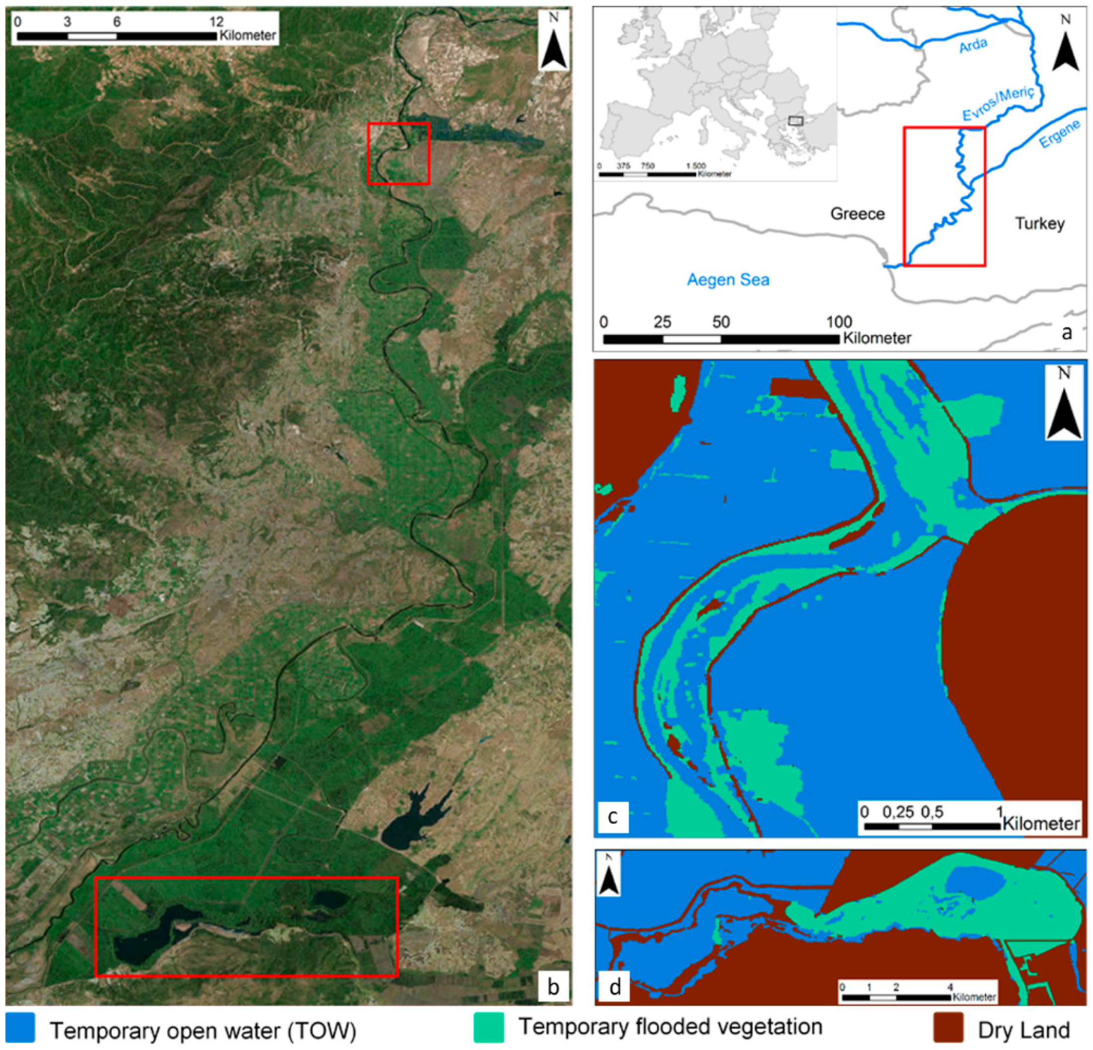
Besides the study area in Namibia described in [8], two further study areas with different vegetation types were used for the impact analysis of time series features for the extraction of TFV. Compared to [8] and to each other, both study areas have different vegetation types, which are described in this section. One of the study areas is part of the Evros catchment, located at the border between Greece and Turkey (Figure 1a) is one of the study areas.
With a length of 515 km and a basin of about 52,900 km2, the Evros river represents the second largest river in Eastern Europe. The period of highest discharge usually occurs between December and April. Several severe, large-scale floods frequently hit the catchment area, particularly in the southern part. The focus of the study lies on a flood event in spring 2015. The flood-affected areas consisted of farmland and forested areas where the water remained for over several weeks. For the analysis and classification, a time series of 60 dual-polarized S-1 scenes was used, which were acquired under the same orbital conditions between October 2014 and December 2016 (Table 1). Five S-1 images covered the flood event. Figure 1b shows the extent of the northern and southern areas of interest, where two scenes, acquired on March 12, 2015 and April 5, 2015 were considered for classification as flood event images due to their temporal proximity to reference data for the two different areas. The northern area is dominated by TFV consisting of deciduous forest, whereby the majority of agricultural fields are entirely inundated during the flood event. In the southern part of the study area, TFV occurs mostly in high grassland areas.
Validation of the classification was performed based on two reference masks (Figure 1c,d). The generation of the reference data was carried out by visual interpretation and manual digitalization of high-resolution optical WorldView-2 (Figure 2) and RapidEye (Figure 3) images, acquired on March 11, 2015 and April 4, 2015, respectively. Although the radar data and the optical image have a temporal shift of one and two days respectively, no changes in the flood extent could be observed.
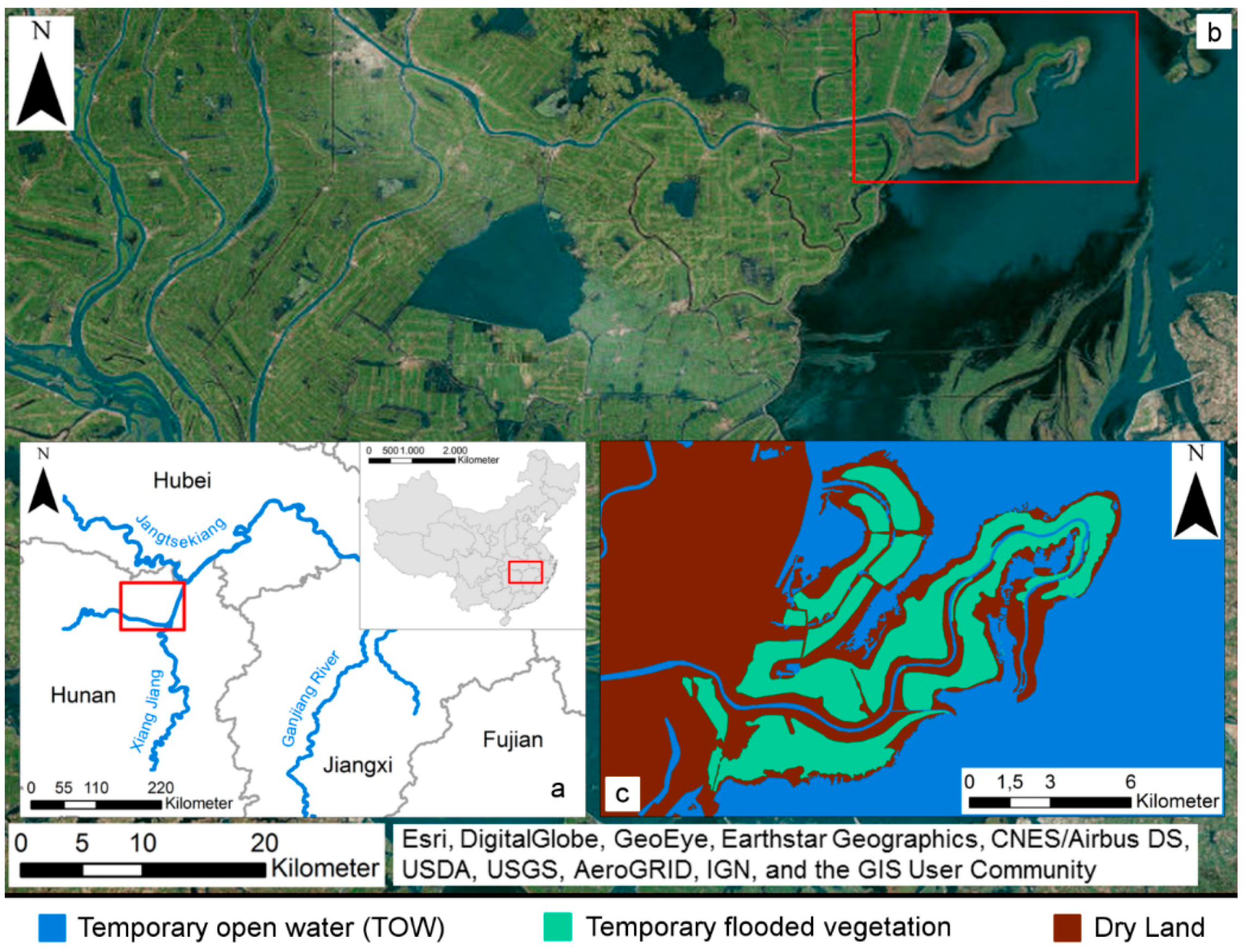
The second test case is the Dong Ting Lake, which is the second largest lake in China, located in the Hunan Province (Figure 4a). It is a flood-basin of the Yangtze River and thus varies seasonally in size. During the annual floods, it can expand to 2691 km2 three times its size compared to the dry season. A flood event in summer 2017 (Figure 4b) was chosen. For this study, 38 dual-polarized S-1 scenes were used, which were acquired between October 2016 and February 2018 (Table 2). The scene acquired on June 28, 2017 is characterized by the largest flood extent. In addition, the selection of the analyzed flood image is carried out due to the temporal proximity to the reference data. Comparable to the study area in Greece/Turkey, the generation of the reference flood mask was carried out using a high-resolution optical Sentinel-2 (S-2) image (Figure 5), which was acquired on June 27, 2017 (Table 2). For the derivation of the reference mask, all bands with a resolution of 10 m and their combinations of the S-2 scene were used. The reference extent and the digitalized reference mask is shown in Figure 4c. No changes in flood extent were observed between the analyzed flood image and the optical scene.
According to the ESA (European Space Agency) acquisition plan for S-1 constellation, dual-polarized images of the S-1A with an interval of 12 days were available for the study areas and the analyzed acquisition period. These data sets are processed and provided by ESA as Ground Range Detected High Resolution (GRDH) products. According to [8], an automated preprocessing of the time series data for both areas and both polarizations VV and VH (vertical/horizontal) was carried out in several steps. The characteristics of all used S-1 data are listed in Table 3.
In addition to the satellite data, ancillary information was used to avoid misclassification of the desired flood-related classes [8] in both study areas. Initially, permanent open water (POW) surfaces were identified by the 30 m SRTM Water Body Data (SWBD) [53]. Besides POW, information regarding urban areas and topography was integrated by using the Global Urban Footprint (GUF) and Height Above Nearest Drainage (HAND) index. Urban areas, as well as TFV, are characterized by strong double- and multiple-bounce backscattering effects. Therefore, the GUF [54] mask is used to identify and exclude urban areas. In order to prevent misclassifications in elevated areas, the HAND index [55] was used to identify and exclude areas with an elevation of greater than 20 m above the nearest water network [56].
2.2. Methodology
The foundation for the analysis of the impact of time series features on the flood extent derivation is the SAR time series approach [8]. This method provides the opportunity to generate flood maps including the classes TOW, TFV and Dry Land (DL) based on different time series features. The main steps of the classification process for the generation of the flood maps are summarized below.
The S-1 time series data presented in Section 2.1 provide a foundation for the generation of two independent multi-temporal layer stacks for each polarization and for each study area via an image preprocessing step. In addition, three further multitemporal stacks are generated, including the combinations of polarization (VV + VH, VV − VH, VV/VH). The ratio between VV and VH was calculated by using linear units, whereby for the elimination of outliers (e.g., due to speckle) only the values within the 5th and 95th percentiles were considered.
Based on findings about characteristics and patterns for TOW and TFV [8], the time series features were determined using the z-transform of the backscatter values for each pixel over the time series and for the available multi-temporal layer stack. The z-transform allows the normalization of the backscatter values over the time series and ensures that the image elements of the analyzed flood scene are comparable with each other when considering the individual seasonal fluctuation of vegetation. The normalized time series features are termed as Z-Score. In relation to the polarizations, the time series features are Z-Score VV, Z-Score VH, the combination of polarization, Z-Score VV + VH, Z-Score VV − VH and the ratio Z-Score VV/VH, which represent the foundation for the derivation of TOW and TFV [8]. Based on training data, two time series features with the highest contribution for the derivation of the desired classes (TOW and TFV) were identified for each study area by using Random Forest Algorithm. These features were used in the last step of the classification approach.
The classification of the flood-related classes was carried out based on pixels and objects. The K-means clustering algorithm [57] was applied for the generation of clusters using SAR time series data and the analyzed flood image. The resulting multitemporal and spatial cluster images were intersected with each other to combine multi-temporal and spatial information. The time series features, which are based on pixels, were merged with the segmented image by averaging the corresponding values within each object.
The hierarchical thresholding approach is the last step in the classification process chain, which allows a successive derivation of the desired classes based on the image elements (pixels or segments). First of all, the permanent water surfaces are identified by the SWBD mask (see Section 2.1). On the remaining image elements, the TOW, TFV and Dry Land (DL) are then derived consecutively using the relevant time series features. The corresponding thresholds were determined automatically using the decision tree classifier and the above-mentioned training data. For further details and an in-depth explanation see [8]. The implementation of the entire approach was done in Python. The quantification of the classification accuracy of TOW, TFV, and DL was carried out using overall accuracy (OA), producer accuracy (PA), user accuracy (UA), and kappa index (K).
In order to investigate the impact of time series features for the derivation of TFV and to show the potential of time series features for the transferability to different study areas and thus for the operational use, a statistical comparison of the classification accuracies based on different study areas and TFV types was performed. Thereby, a single time series feature was searched for, which allows the extraction of different types of TFV with high accuracy for all study areas. Besides the study areas described in Section 2.1, the study area in Namibia, which was analyzed in Tsyganskaya et al., [8], was also used for the investigation.
In order to identify a single time series feature, which can then be used for all study areas, the mean value and the coefficient of variation (CV) were determined based on user accuracy (UA) and producer accuracy (PA) for each time series feature. The mean value represents the total accuracy for the TFV classification of all study areas and for each time series feature. The higher the mean value, the more relevant is the time series feature for all study areas. In addition, the CV was used to quantify the variance of the data relative to the mean. The variance of the values is particularly relevant with regard to the outliers in UA and PA. The lower the CV, the lower the distance/scatter between the classification accuracies of the study areas for a time series feature and the more relevant is a time series feature for all study areas and thus for their transferability. Thus, the two statistical quantities allow the comparison between the classification results and the time series features for all study areas simultaneously.
3. Results and Discussion
3.1. Level of Contribution of the Time Series Features
Based on the knowledge about the characteristics and patterns of the time series data for the two polarizations and their combinations, time series features were derived [8]. Using training data for each of the study areas, those features were examined for their relevance to the extraction of the desired classes, TOW and TFV. For this purpose, similarly large training data sets were derived from optical images for the three classes TOW, TFV, and DL and for each of the study areas. Using Random Forest Algorithm, it was identified which time series features provide the highest contribution to the classification results and are, therefore, most relevant for the derivation of flood-related classes. Furthermore, it was examined whether a single time series feature or a combination of time series features enables the highest classification accuracy for the two desired classes. As a result, redundant information can be sorted out and the information required for classification identified.
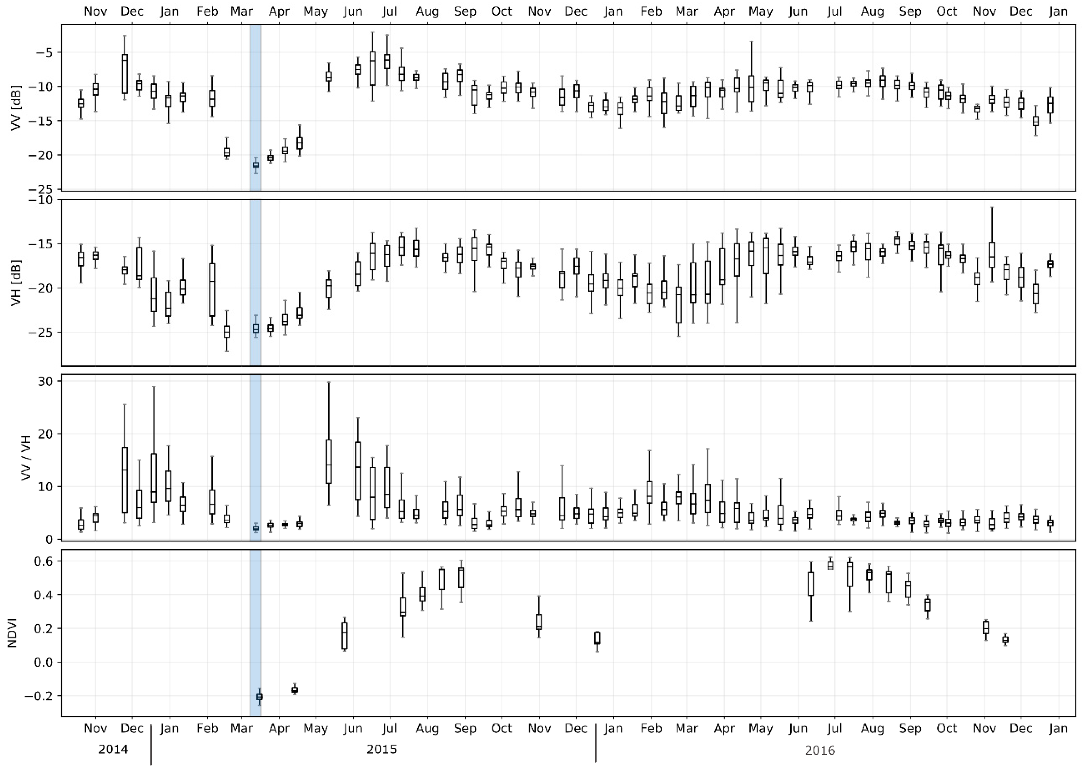
Table 4 and Table 5 show the level of contribution of the analyzed time series features for the derivation of the above-mentioned classes and the three study areas. Z-Score VV + VH represents the time series feature with the highest contribution for TOW for all study areas (Table 5). This can be explained by the fact that for both VV and VH polarizations the backscatter values decrease at the analyzed date of the flood [8]. An example of the backscatter value decrease in VV and VH is shown in Figure 6, which was created for a TOW segment from the validation data. Z-Score VV + VH combines both sources of information, whereby the decrease of the backscatter values is intensified. Figure 2b shows the enlarged view of the high-resolution WorldView2 image, demonstrating the presence of the corresponding TOW at the analyzed flood date. Further examples of TOW and the analyzed extent of study areas in southern Greece/Turkey and China are demonstrated in Figure 3a and Figure 5c. In addition to both polarizations, the multi-temporal behavior of the Normalized Difference Vegetation Index (NDVI) values for the same time-period is displayed in Figure 6 serving as a comparison to the SAR time series data. NDVI values were derived from the LANSAT 8 data sets. Despite the cloud-related data gap for 2014, the beginning of 2015 and the beginning of 2016, a strong decrease in the NDVI values for the analyzed date of the flood event can be observed. In combination with the decrease of the backscatter values, this confirms the occurrence of water at the analyzed date. For the classification of TFV, different time series features with the highest contribution or relevance can be identified for the individual study areas. The differences can be attributed to the different types of vegetation and the different environmental conditions in the study areas.
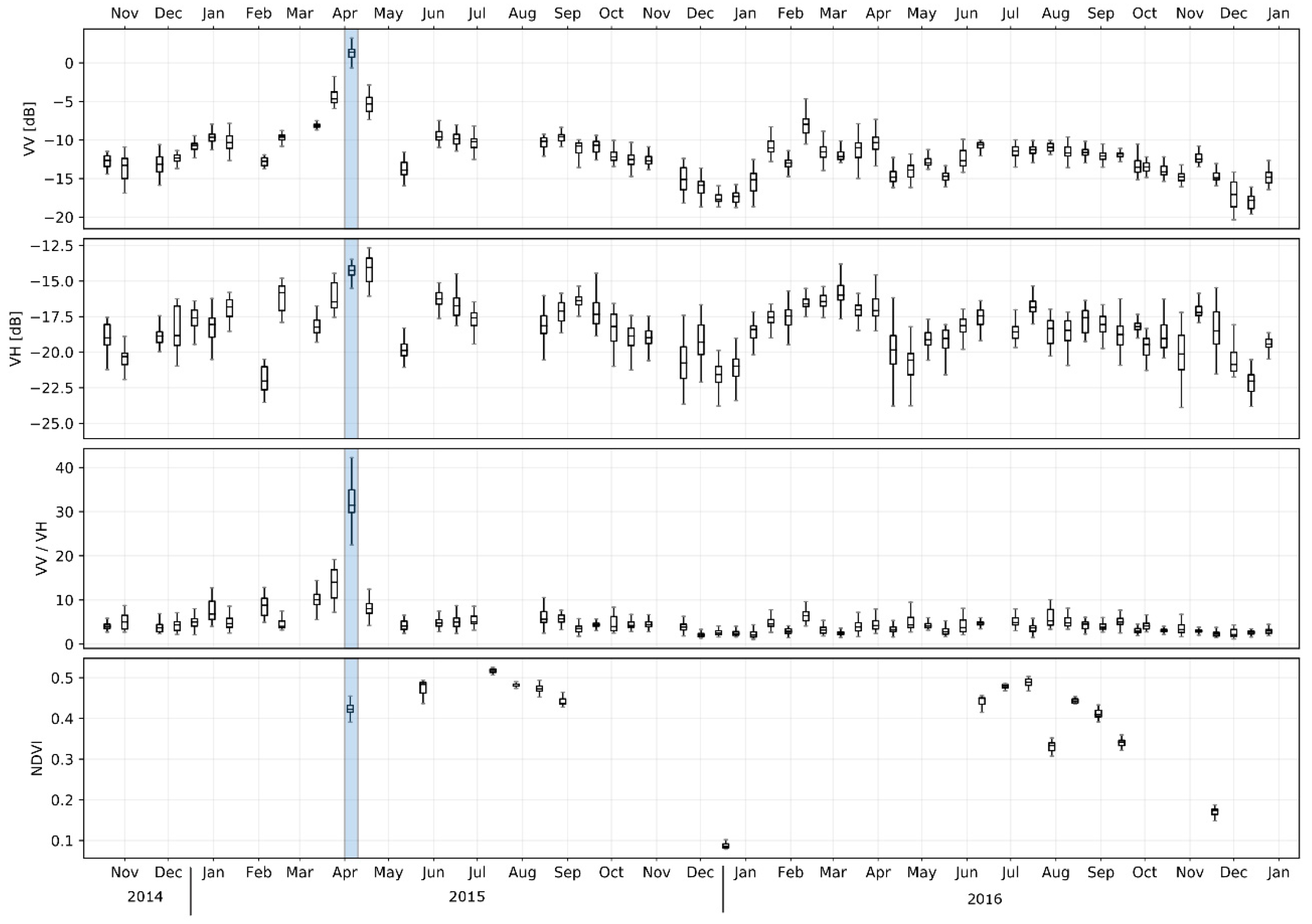
For the study area in southern Greece/Turkey, the Z-Score VV − VH is the most relevant time series feature for the derivation of TFV (Table 5). This can be explained by the strong difference between the polarizations VV and VH (Figure 7). Thereby, VV polarization shows a strong increase at the flood date compared to the rest of the time series and VH polarization shows low or almost no increase at the flood date.
The different behavior of both polarizations can be explained by the different sensitivity of VV and VH to specific backscattering mechanisms, which caused an increased difference in the backscatter values between the two polarizations at the analyzed date of the flood. In comparison, the difference between the polarizations for the dry dates shows a smaller variability. The different sensitivity is on the one hand due to the fact that the double-bounce effect occurs more strongly in the VV polarization and leads to the backscatter. On the other hand, backscatter is in general lower for cross-polarization (HV or VH), as no ideal corner reflectors can be produced due to their depolarizing properties [5,58,59]. As a result, it is reported that the increase of the backscatter values by TFV can be more reliably detectable by co-polarized data than by cross-polarized data [60]. However, the combination of co- and cross-polarized data can improve the identification of TFV [26]. The NDVI values in Figure 7 confirm that the increase in VV polarization was not caused by seasonal or other changes in vegetation, but is flood-related, as no sudden increase in NDVI values could be identified at the flood date.
For the study area in northern Greece/Turkey, Z-Score VV is the most relevant feature (Table 5). As previously mentioned in Section 2.1, this study area is dominated by deciduous forest (Figure 2a), which was under leaf-on conditions at the date of the flood. It should be noted that the penetration of the forest canopy may be restricted by C-band and environmental parameters (e.g., aboveground biomass) [61,62]. Yu and Satschi [63] reported that the SAR backscatter values increase depending on the biomass and that the soil signal can no longer be detected if a certain degree of saturation has been reached. Thereby, the volume scattering from the canopy completely superimposes the contribution of the double bounce effects from the interaction between the water surface and vertical vegetation structure and TFV can no longer be identified. Therefore, there is hardly any signal difference between VV and VH at the flood date (Figure 8), which is confirmed by the low importance of Z-Score VV − VH. Compared to that the small increase in importance of the VV/VH can be explained by a small proportion of TFV in the forested areas due to limited penetration into the forest crown, as described above. In the case of northern Greece/Turkey the importance increases, because the outliers were eliminated by using the Z-Score VV/VH feature. For southern Greece/Turkey on the contrary, using the Z-Score VV/VH the outlier reduction caused also an elimination of extreme values caused by TFV. This led to a drop of the importance in VV/VH in comparison to the Z-Score VV − VH. Regarding the most relevant time series feature Z-Score VV for the northern Greece/Turkey study area, it is assumed that the backscatter in VV polarization is dominated by the contribution of the forest canopy and moreover the volume scattering represents the main scattering mechanism. Due to the sensitivity of the VV polarization for the double bounce effect, however, a slight increase in the backscattering values at the flood date was detected, which can indicate TFV (Figure 8). The NDVI values were derived from the LANDSAT 8 data and show that the slight increase of the backscatter values in both polarizations at the date of flood can be attributed to the flood event and not to any change in vegetation.
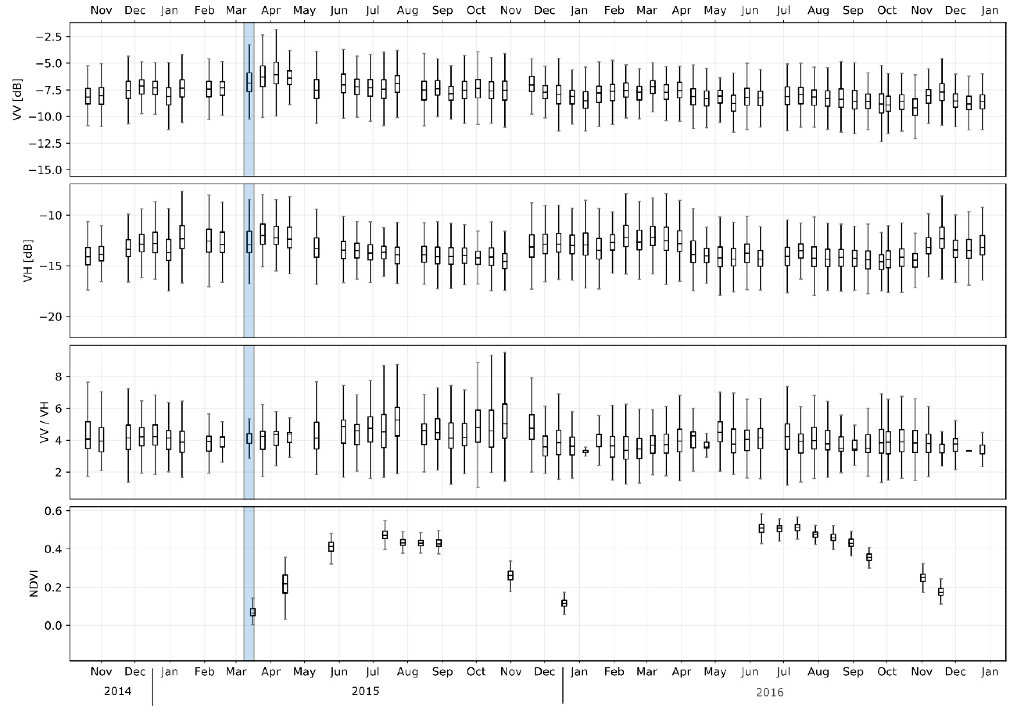
For the study area in China, Z-Score VV + VH represents the most relevant time series feature for the derivation of the TFV (Table 5). The time series feature indicates that in both polarizations an increase of the backscatter values has occurred at the analyzed date of the flood. This can be confirmed in Figure 9. Both polarizations increase at the analyzed flood date, whereas the stronger increase can be observed in VV polarization. The sum of the two polarizations intensifies the increase of the backscatter values at the same date. Although only a few cloud-free optical Sentinel-2 images are available that cover the study area in China for the analyzed time period, it can be observed that there is no increase in the NDVI values at the analyzed flood date (Figure 9). This leads to the deduction that the increase in SAR time series data is not related to phenological changes. Figure 5b shows a high-resolution Sentinel-2 image demonstrating the presence of the corresponding TFV area at the analyzed flood date.
Since the TFV type is high grassland and reed (Figure 5b) [64], which is similar to the structure of some crops (rice, wheat), it is assumed that the vegetation can be penetrated by the C-band data [10,65]. Therefore, it is expected that the increase in backscatter values will occur at the time of the flood in the VV polarization due to their sensitivity to the double impact effect. However, the increase in VH polarization cannot be confirmed by the depolarizing property mentioned above. Instead, the latter increase is a result of the combination of environmental parameters. The contribution of the soil under the vegetation plays a decisive role in this process. Due to of possible unevenness of the soil (microtopography) and the low water level, it is possible that a part of the soil surface beneath the vegetation was only partially flooded. In the flood-free areas underneath the vegetation, the soil moisture may have increased at the date of the flood compared to non-flooded conditions. Simultaneously, water could have accumulated in the sinks, which could also lead to standing water beneath vegetation in the same region. Due to different sensitivities of VV and VH to the respective conditions, the latter can dominate the respective polarization. The analyses from the literature confirm that an increase in soil moisture in both VV and VH causes an increase in the backscatter values and can be detected by the sensor depending on the biomass amount [66,67]. The TFV, which is represented by the double-bounce effect, can only be detected by VV polarization, as the depolarizing property of VH polarization does not allow sensitivity to double-bounce [68]. The mixture of these two cases by micro topographical differences explains the increase not only of backscatter values for VV, but also for VH and, thus, the relevance of Z-Score VV + VH for the derivation of TFV in the study area of China.
A comparison of the relevant time series features with the results of the study of Tsyganskaya et al., [8] shows that for the class TOW, Z-Score VV + VH is also one of the time series features with the highest contribution. For TFV, the most relevant time series characteristic (Z-Score VV − VH) is confirmed only for the study area in the southern area of interest of Greece/Turkey. In the other two example areas, the algorithm determined different relevant time series features due to different environmental conditions (e.g., vegetation type, topography, soil moisture) and their interaction.
Based on a previous analysis in Tsyganskaya et al., [8], the time series feature with the highest contribution can achieve a higher classification accuracy compared to the combination of all time series features. Therefore, a single time series feature with the highest contribution was used for the classification for deriving the desired classes. This identification step is performed automatically by the algorithm using training data. Moreover, these examples show that the use of both polarizations is relevant for the derivation of flooded areas.
3.2. Classification Results
The classification of the study area in southern Greece/Turkey was carried out based on the S-1 time series stack (October 19, 2014–December 25, 2016) containing the flood image (April 4, 2015). This classification was validated using the S-2-based reference mask (April 5, 2015). Figure 10a shows the pixel-based classification result of the time series approach, which comprises the classes POW, TOW, TFV, and DL, while Figure 10b shows the object-based classification result. For visual comparison, the validation mask is shown in Figure 1d. It is noticeable that the areas of the classes TOW, TFV, and DL contain more small structures of the other classes in the pixel-based classification compared to the object-based classification. The usage of objects reduces this noise; however, it also can lead to the loss of details and thus information. In general, the use of pixel- or object-based classification depends strongly on the kind of the landscape under investigation. In the case of flooding in vegetated areas, a single, isolated pixel could contain water ponds and so differ from its neighboring pixels. Due to limited visibility in optical data, these areas could not be identified during the generation of the validation mask.
For the study area in northern Greece/Turkey, the classification is based on the S-1 time series stack (October 19, 2014–December 25, 2016), with the flood image being acquired on March 12, 2015. Validation of this classification was performed using the S-2-based reference mask (March 15, 2015). Figure 11a shows the pixel-based classification result for the study area of northern Greece/Turkey, which comprises the classes POW, TOW, TFV, and DL, while Figure 11b shows the object-based classification result. Compared to the validation mask (Figure 1c), both pixel- and object-based classification show only a low representativity of the class TFV. This can be explained by the low penetration of the vegetation (deciduous forest (Figure 2a)) by the C-band data, which is reduced in this case [8]. In addition, occasional TFV areas in the classification can be identified in DL of the validation mask, especially in the pixel-based classification. These could be small areas of water (ponds or temporary water accumulations). In combination with vertical structures of the agricultural areas or grassland, the double bounce effect can also be produced resulting in an increase in the backscatter values at the date of the flood. These areas were also classified as TFV, though they could not, however, be identified during the generation of the validation mask due to limited visibility in optical data.
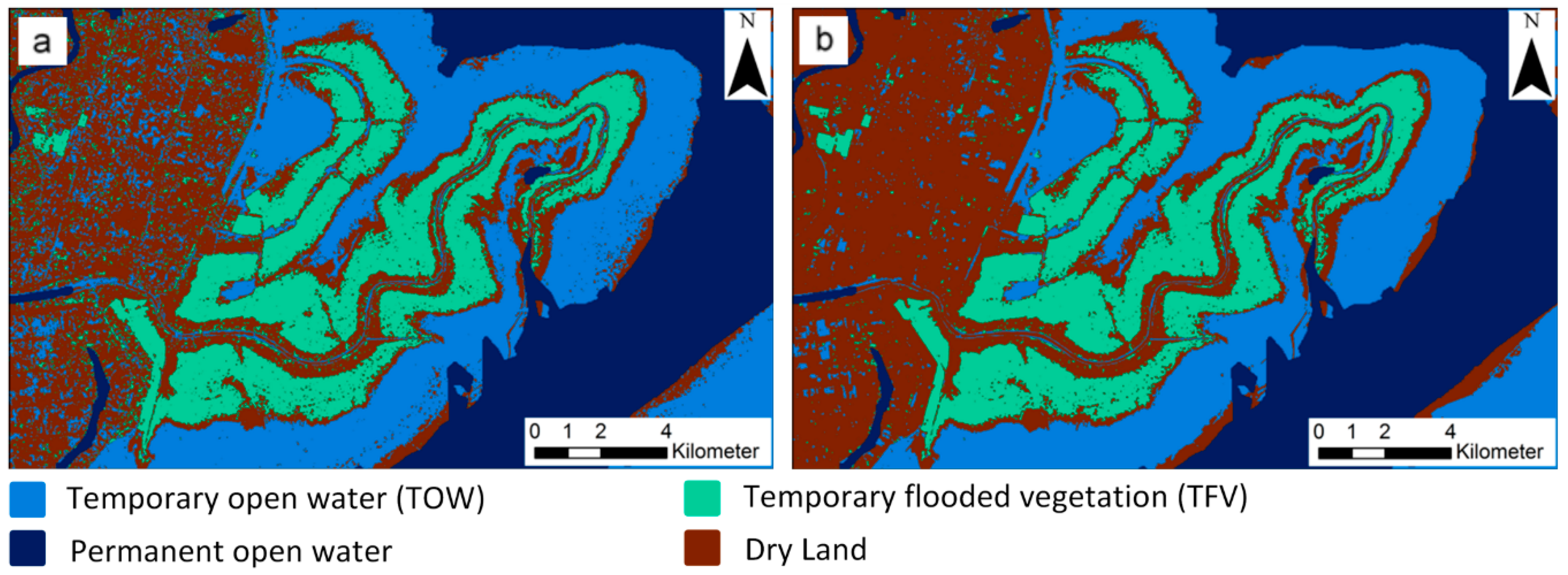
The classification for the study area in China was performed using the S-1 time series stack (October 19, 2016–February 23, 2018). The analyzed date of the flood is June 28, 2017. The validation for this classification was performed using the S-2-based reference mask (June 27, 2017). Figure 12a, b show the pixel- and object-based classification results with POW, TOW, TFV, and DL classes. The validation mask used is shown in Figure 4c.
The comparison between the classification results and the validation mask reveals the occurrence of TOW in DL. DL also occurs between the permanent water surfaces and the TOW areas. On the one hand, the confusion between these two classes can arise due to small areas of water occurring in the agricultural areas. On the other hand, the duration of a flood event can lead to an accumulation of S-1 images, containing the inundation and a decrease of images without flooding. This can cause a higher fluctuation range and a lower mean value when generating the time series features, which in particular can lead to confusion with DL, as the areas between permanent water and TOW demonstrate. The combination of these two conditions makes the above-mentioned confusions between the classes possible. Therefore, the use of a time series with at least one vegetation cycle is recommended, as the statistical range of the backscatter values of the vegetation stages is detected and thus sufficiently represented [8].
The accuracy values for the pixel-based and object-based classifications for the respective study areas are shown in Table 6. The OA for all study areas ranges between 80% and 87%. In comparison, in [8] the authors achieved a similar or even slightly lower OA for the pixel-based (75%) and object-based (82%) classification. The accuracy assessment for the study area in northern Greece/Turkey shows high values for the TOW class but strong misclassifications for TFV (PA: 28% for pixel-based and 6% for object-based) and DL (UA: 57% for pixel-based and 53% for object-based). This indicates a significant confusion between these two classes and can be explained by different environmental conditions (see Section 3.1). The accuracy values show no significant difference between pixel-based and object-based classification, except for the PA values of TFV. When applying object-based classification, it should be noted that the small-scale flood areas could be generalized by merging the pixels to objects. However, object-based classification can help to exclude pixels which can be confused with a flood-related increase in values due to dominant environmental conditions, such as soil moisture, topography, or surface roughness, which can cause a small-scale increase or decrease in the backscatter. In addition, objects are less susceptible to speckle noise than pixels [29].
3.3. Time Series Features—Transferability Analysis
For the transferability analysis of the classification approach, several pixel-based and object-based classification runs were carried out for each study area and its subareas using the individual time series features. For each run, the most relevant time series feature (Z-Score VV + VH) was used for the derivation of TOW (Section 3.1). Simultaneously, each time series feature was used in each study area to derive the TFV, so that 20 pixel-based and 20 object-based classification products could be generated. For each result, an accuracy assessment was performed. Since the analysis of the different time series features refers to the TFV, the PA and UA of TFV were selected as indicators to represent the classification accuracy of the TFV. The accuracy values PA and UA for the individual study areas and the five analyzed time series features for pixel-based classification are shown in Table 7 and for object-based classification in Table 8. The relevant time series features that were identified by the Random Forest Algorithm (Section 3.1) are highlighted in dark green for the respective study areas for the PA and UA values. These tables show that different time series features are relevant for the individual study areas. The low PA values seen for northern Greece in both tables can be explained by the specific TFV type that dominates this study area, namely flooded forest areas. In this case, the penetration of the forest crown is limited by C-band data, whereby the water under the vegetation can only be partially detected.
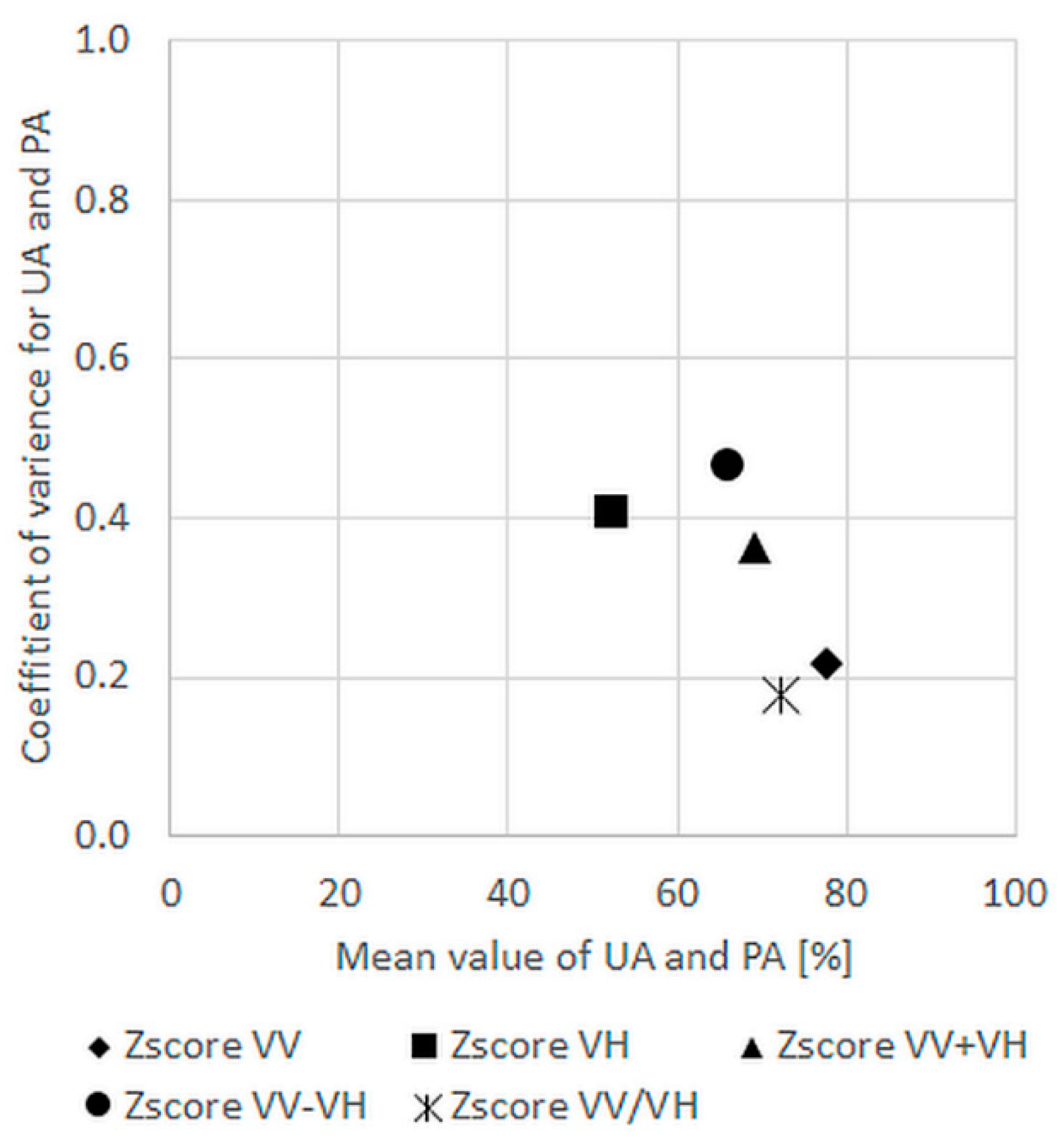
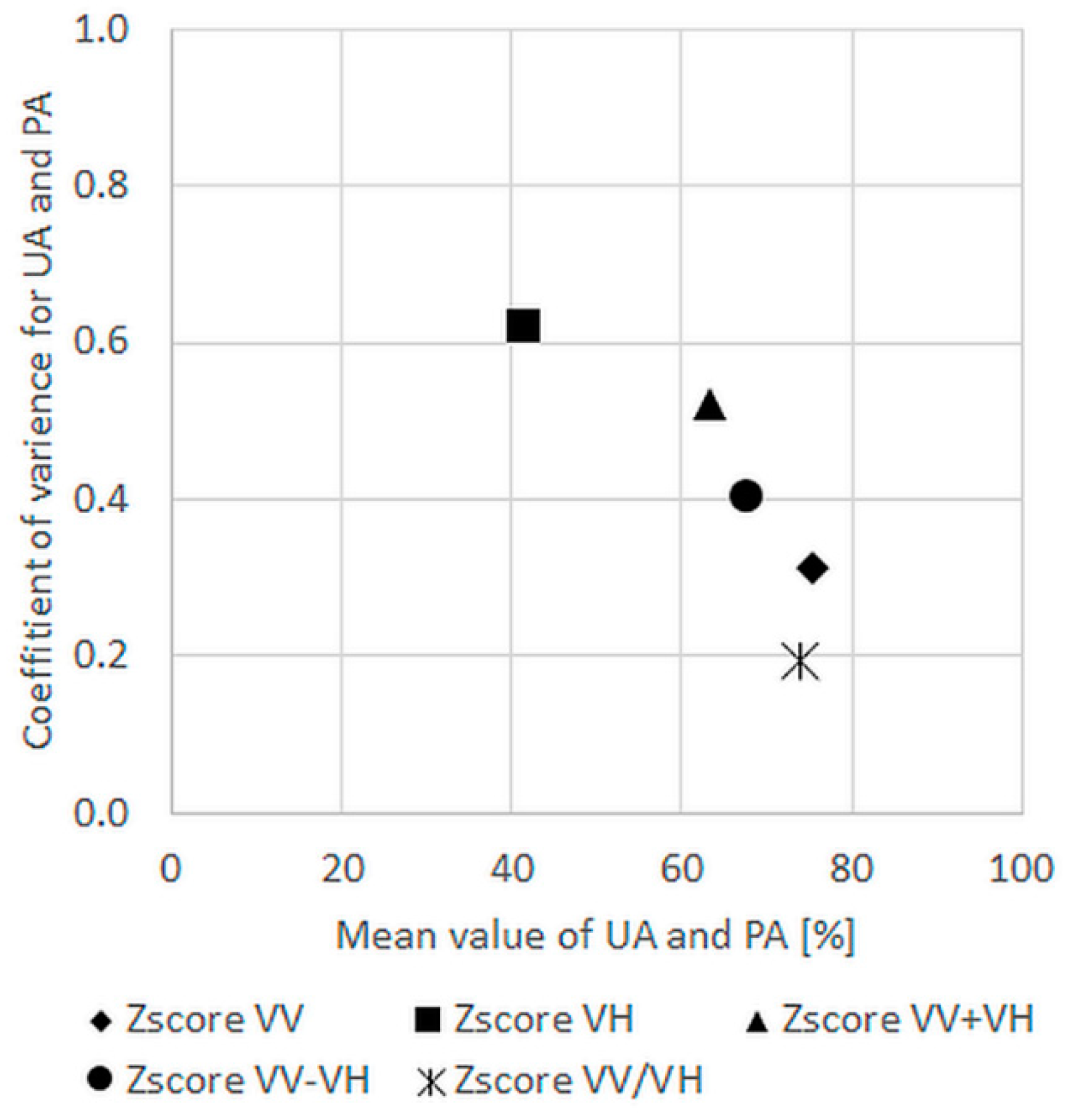
As described in the methodology, two quantities, mean value and CV, were derived based on the UA and PA values to provide a foundation for the identification of a single robust time series feature for the derivation of TFV types and for all study areas. If a time series feature reaches a high mean value compared to other time series features and shows at the same time the smallest CV, it is relevant for all study areas. Considering Table 7 and Table 8, it is not apparent which time series feature would be suitable since the two statistical variables achieve the optimum at different time series features (highlighted in light green). The Z-Score VV shows the highest mean value (77.54%) for pixel-based classification and (75.57%) for object-based classification compared to other time series features, but Z-Score VV/VH shows the lowest CV value (0.18) for pixel-based and (0.19) for object-based.
For a distinct identification of the most relevant time series feature, the two statistical variables have to be considered simultaneously. In Figure 13, the two quantities are plotted on two different axes. The larger the mean value and the smaller the CV, the more suitable is a time series feature for the extraction of TFV for all study areas. The lower right corner of the diagram is thus the point that represents the optimum between both statistical quantities. The closer a time series feature lies to this optimum, the more relevant is the time series feature for all study areas.
Compared to other time series features, Z-Score VV is the shortest regarding the distance between the optimum and the time series feature for pixel-based classification (Figure 13). Thus, this time series feature seems to be the most relevant for the operational derivation of the class TFV, when using pixels as a foundation. The relevance of Z-Score VV is due to the fact that VV polarization is more influenced by the double-bounce effect indicating the presence of TFV. In comparison, VH is more influenced by different environment conditions and may change for different TFV types and study areas (Section 3.1). The distances of the Z-Score VV/VH to the optimal point differ from the distance between the Z-Score VV and optimal point only slightly. This shows that VH polarization also has an influence on the classification results and can be important in combination with VV polarization provided that the environmental conditions in the analyzed study area are known and characterized.
This relevance is also shown in Figure 14, where the relevant feature based on objects is the Z-Score VV/VH, which contains both polarizations. Based on the findings in Section 3.1, which show that the increase in the VV time series at the date of the flood for TFV is more significant compared to the VH time series because the VH signal is influenced more by environmental conditions than by TFV, the Z-Score VV feature based on pixel elements is recommended for operational use. In addition, the mean value of UA and PA for the pixel-based classification for the Z-Score VV time series feature is highest (77.54%) compared to all other mean values of UA and PA. The combination of Z-Score VV + VH and Z-Score VV/VH based on pixel elements is recommended for operative use for extraction of the TOW and TFV, respectively. When no feature importance has to be calculated during the classification and the pre-processing of the S-1 data [8] has already taken place, the classification process takes between 1 and 5 minutes, depending on the available computing performance and the extent of the study area. The maximum extent that was analyzed is one-third of S-1 GRD images. By specifying the time series features the user, interaction is omitted and apart from the initialization of the algorithm the classification can be performed automatically. For the optimization and extension of the approach regarding different TFV types, further research in other study areas will be beneficial.
4. Conclusions
The results of the study areas in northern and southern Greece/Turkey and in China show the potential of the method presented in Tsyganskaya et al., [8] using S-1 time series data to extract the total flood extent considering both temporary open water (TOW) and temporary flooded vegetation (TFV). In particular, different types of TFV were analyzed. The individual flood extent was determined by time series features, which represent the characteristics of both classes.
This study confirms the results of the study of Tsyganskaya et al., [8], showing that the Z-Score VV+VH, which was derived based on the characteristics mentioned above, is the most relevant time series feature for the extraction of the TOW areas in all study areas. For the derivation of TFV, three different time series features were determined by the algorithm for individual study areas. This can be explained by the complex structure of the vegetation, the various analyzed vegetation types, and the dependency of the TFV on environmental conditions (e.g., vegetation type, soil moisture, topography), which differ in all study areas. Nevertheless, in the results for all study areas OA values reached between 80% and 87%, which were slightly higher even compared to the results in [8]. For the study area in northern Greece, the TFV areas could only partially be derived based on the C-band data due to the presence of forested vegetation, which reduces the penetration of the SAR signal. In both other study areas, TFV in high grassland/reed was successfully classified.
The potential of the time series approach for transferability as a prerequisite for operational use was analyzed by comparing time series features with respect to their suitability for the derivation of TFV for all study areas simultaneously. For the comparison, statistical quantities were derived from the classification accuracies PA and UA of the TFV. For TFV, Z-Score VV, or Z-Score VV/VH appear to be the most relevant time series feature for pixel-based and object-based classification, respectively. Nevertheless, Z-Score VV is recommended for operational use based on pixel elements for the extraction of TFV as this allows improved differentiation to non-flood dates due to the more significant increase in the VV time series for TFV at the date of the flood compared to the VH time series. The Z-Score VV + VH is recommended for the extraction of TOW surfaces, because of the unanimity regarding the feature importance calculation for all study areas (Section 3.1). Since the time series features have been defined and no feature importance needs to be calculated, the user interaction is reduced to the initialization of the classification process and the computation time decreases.
Overall, the approach can be used for irregularly occurring flood events, as well as for irregularly acquired S-1 images. It is flexible for individual applications depending on the vegetation and takes account of the seasonal changes by the use of multitemporal data. The presented SAR time series approach lays the cornerstone for automatic flood detection on a global scale, allowing the detection of the entire flood extent by supplementing the TOW with TFV areas.
Author Contributions
The concept of this study was developed by V.T., P.M. and S.M., while V.T. was responsible for the implementation, which included the preparation of data, generation and validation of flood classification maps, and methodological comparison of relevant features and their discussion.
Funding
This work is funded by the Federal Ministry for Economic Affairs and Energy (BMWi), grant number 50 EE1338.
Acknowledgments
The WorldView-2 imagery was kindly provided by European Space Imaging Ltd. (EUSI). The RapidEye imagery was kindly provided by Planet Labs Inc.
Conflicts of Interest
The authors declare no conflict of interest.
References
- The International Disaster-Emergency Events Database (EMDAT). OFDA/CRED International Disaster Database; Université catholique de Louvain: Brussels, Belgium, 2019; Available online: https://www.emdat.be (accessed on 1 August 2019).
- Centre for Research on the Epidemiology of Disasters (CRED); The United Nations Office for Disaster Risk Reduction (UNISDR). 2018 Review of Disaster Events. 2019. Available online: https://www.emdat.be/publications (accessed on 31 August 2019).
- Klemas, V. Remote Sensing of Floods and Flood-Prone Areas: An Overview. J. Coast. Res. 2014, 31, 1005–1013. [Google Scholar] [CrossRef]
- Cazals, C.; Rapinel, S.; Frison, P.-L.; Bonis, A.; Mercier, G.; Mallet, C.; Corgne, S.; Rudant, J.-P. Mapping and Characterization of Hydrological Dynamics in a Coastal Marsh Using High Temporal Resolution Sentinel-1A Images. Remote Sens. 2016, 8, 570. [Google Scholar] [CrossRef]
- Martinis, S.; Rieke, C. Backscatter Analysis Using Multi-Temporal and Multi-Frequency SAR Data in the Context of Flood Mapping at River Saale, Germany. Remote Sens. 2015, 7, 7732–7752. [Google Scholar] [CrossRef] [Green Version]
- Pulvirenti, L.; Pierdicca, N.; Chini, M. Analysis of Cosmo-SkyMed observations of the 2008 flood in Myanmar. Ital. J. Remote Sens. 2010, 42, 79–90. [Google Scholar] [CrossRef]
- Brisco, B.; Shelat, Y.; Murnaghan, K.; Montgomery, J.; Fuss, C.; Olthof, I.; Hopkinson, C.; Deschamps, A.; Poncos, V. Evaluation of C-Band SAR for Identification of Flooded Vegetation in Emergency Response Products. Can. J. Remote Sens. 2019. [Google Scholar] [CrossRef]
- Tsyganskaya, V.; Martinis, S.; Marzahn, P.; Ludwig, R. Detection of Temporary Flooded Vegetation Using Sentinel-1 Time Series Data. Remote Sens. 2018, 10, 1286. [Google Scholar] [CrossRef]
- Moser, L.; Schmitt, A.; Wendleder, A. Automated Wetland Delineation from Multi-Frequency and Multi-Polarized SAR Images in High Temporal and Spatial Resolution. ISPRS Ann. Photogramm. Remote Sens. Spat. Inf. Sci. 2016, 3, 57–64. [Google Scholar] [CrossRef]
- Pulvirenti, L.; Pierdicca, N.; Chini, M.; Guerriero, L. Monitoring Flood Evolution in Vegetated Areas Using COSMO-SkyMed Data: The Tuscany 2009 Case Study. IEEE J. Sel. Top. Appl. Earth Obs. Remote Sens. 2012, 6, 1807–1816. [Google Scholar] [CrossRef]
- Betbeder, J.; Rapinel, S.; Corpetti, T.; Pottier, E.; Corgne, S.; Hubert-Moy, L. Multitemporal Classification of TerraSAR-X Data for Wetland Vegetation Mapping. J. Appl. Remote Sens. 2014, 8, 83648. [Google Scholar] [CrossRef]
- Chapman, B.; McDonald, K.; Shimada, M.; Rosenqvist, A.; Schroeder, R.; Hess, L. Mapping Regional Inundation with Spaceborne L-Band SAR. Remote Sens. 2015, 7, 5440–5470. [Google Scholar] [CrossRef] [Green Version]
- Evans, T.L.; Costa, M.; Tomas, W.M.; Camilo, A.R. Large-Scale Habitat Mapping of the Brazilian Pantanal Wetland. A synthetic aperture radar approach. Remote Sens. Environ. 2014, 155, 89–108. [Google Scholar] [CrossRef]
- Hess, L. Dual-Season Mapping of Wetland Inundation and Vegetation for the Central Amazon Basin. Remote Sens. Environ. 2003, 87, 404–428. [Google Scholar] [CrossRef]
- Lang, M.W.; Kasischke, E.S.; Prince, S.D.; Pittman, K.W. Assessment of C-band synthetic aperture radar data for mapping and monitoring Coastal Plain forested wetlands in the Mid-Atlantic Region, USA. Remote Sens. Environ. 2008, 112, 4120–4130. [Google Scholar] [CrossRef]
- Chini, M.; Papastergios, A.; Pulvirenti, L.; Pierdicca, N.; Matgen, P.; Parcharidis, I. SAR coherence and polarimetric information for improving flood mapping. In Proceedings of the 2016 IEEE International Geoscience & Remote Sensing Symposium, Beijing, China, 10–15 July 2016; pp. 7577–7580. [Google Scholar]
- Morandeira, N.; Grings, F.; Facchinetti, C.; Kandus, P. Mapping Plant Functional Types in Floodplain Wetlands. An Analysis of C-Band Polarimetric SAR Data from RADARSAT-2. Remote Sens. 2016, 8, 174. [Google Scholar] [CrossRef]
- Touzi, R.; Deschamps, A.; Rother, G. Wetland Characterization using Polarimetric RADARSAT-2 Capability. Can. J. Remote Sens. 2007, 33, S56–S67. [Google Scholar] [CrossRef]
- Pulvirenti, L.; Chini, M.; Pierdicca, N.; Boni, G. Use of SAR Data for Detecting Floodwater in Urban and Agricultural Areas: The Role of the Interferometric Coherence. IEEE Trans. Geosci. Remote Sens. 2016, 54, 1532–1544. [Google Scholar] [CrossRef]
- Baghdadi, N.; Bernier, M.; Gauthier, R.; Neeson, I. Evaluation of C-band SAR Data for Wetlands Mapping. Int. J. Remote Sens. 2001, 22, 71–88. [Google Scholar] [CrossRef]
- Gallant, A.; Kaya, S.; White, L.; Brisco, B.; Roth, M.; Sadinski, W.; Rover, J. Detecting Emergence, Growth, and Senescence of Wetland Vegetation with Polarimetric Synthetic Aperture Radar (SAR) Data. Water 2014, 6, 694–722. [Google Scholar] [CrossRef] [Green Version]
- White, L.; Brisco, B.; Pregitzer, M.; Tedford, B.; Boychuk, L. RADARSAT-2 Beam Mode Selection for Surface Water and Flooded Vegetation Mapping. Can. J. Remote Sens. 2014, 40, 135–151. [Google Scholar]
- Brisco, B.; Schmitt, A.; Murnaghan, K.; Kaya, S.; Roth, A. SAR Polarimetric Change Detection for Flooded Vegetation. Int. J. Digit. Earth 2011, 6, 103–114. [Google Scholar] [CrossRef]
- De Grandi, G.F.; Mayaux, P.; Malingreau, J.P.; Rosenqvist, A.; Saatchi, S.; Simard, M. New Perspectives on Global Ecosystems from Wide-Area Radar Mosaics. Flooded forest mapping in the tropics. Int. J. Remote Sens. 2010, 21, 1235–1249. [Google Scholar] [CrossRef]
- Dabboor, M.; White, L.; Brisco, B.; Charbonneau, F. Change Detection with Compact Polarimetric SAR for Monitoring Wetlands. Can. J. Remote Sens. 2015, 41, 408–417. [Google Scholar] [CrossRef]
- Zhao, L.; Yang, J.; Li, P.; Zhang, L. Seasonal Inundation Monitoring and Vegetation Pattern Mapping of the Erguna Floodplain by Means of a RADARSAT-2 Fully Polarimetric Time Series. Remote Sens. Environ. 2014, 152, 426–440. [Google Scholar] [CrossRef]
- Koch, M.; Schmid, T.; Reyes, M.; Gumuzzio, J. Evaluating Full Polarimetric C- and L-Band Data for Mapping Wetland Conditions in a Semi-Arid Environment in Central Spain. IEEE J. Sel. Top. Appl. Earth Obs. Remote Sens. 2012, 5, 1033–1044. [Google Scholar] [CrossRef]
- Lee, J.-S.; Pottier, E. Polarimetric Radar Imaging: From Basics to Applicationsvol; CRC Press: Boca Raton, FL, USA, 2009; p. 142. [Google Scholar]
- Tsyganskaya, V.; Martinis, S.; Marzahn, P.; Ludwig, R. SAR-based Detection of Flooded Vegetation–A Review of Characteristics and Approaches. Int. J. Remote Sens. 2018, 39, 2255–2293. [Google Scholar] [CrossRef]
- Chini, M.; Pulvirenti, L.; Pierdicca, N. Analysis and Interpretation of the COSMO-SkyMed Observations of the 2011 Japan Tsunami. IEEE Geosci. Remote Sens. Lett. 2012, 9, 467–471. [Google Scholar] [CrossRef]
- Long, S.; Fatoyinbo, T.E.; Policelli, F. Flood Extent Mapping for Namibia using Change Detection and Thresholding with SAR. Environ. Res. Lett. 2014, 9, 035002. [Google Scholar] [CrossRef]
- Voormansik, K.; Praks, J.; Antropov, O.; Jagomagi, J.; Zalite, K. Flood Mapping with TerraSAR-X in Forested Regions in Estonia. IEEE J. Sel. Top. Appl. Earth Obs. Remote Sens. 2014, 7, 562–577. [Google Scholar] [CrossRef]
- Horritt, M.S.; Mason, D.C.; Luckman, A.J. Flood Boundary Delineation from Synthetic Aperture Radar Imagery Using a Statistical Active Contour Model. Int. J. Remote Sens. 2001, 22, 2489–2507. [Google Scholar] [CrossRef]
- Martinis, S.; Twele, A. A Hierarchical Spatio-Temporal Markov Model for Improved Flood Mapping Using Multi-Temporal X-Band SAR Data. Remote Sens. 2010, 2, 2240–2258. [Google Scholar] [CrossRef] [Green Version]
- Chen, Y.; He, X.; Wang, J.; Xiao, R. The Influence of Polarimetric Parameters and an Object-Based Approach on Land Cover Classification in Coastal Wetlands. Remote Sens. 2014, 6, 12575–12592. [Google Scholar] [CrossRef] [Green Version]
- Plank, S.; Jüssi, M.; Martinis, S.; Twele, A. Mapping of Flooded Vegetation by Means of Polarimetric Sentinel-1 and ALOS-2/PALSAR-2 imagery. Int. J. Remote Sens. 2017, 38, 3831–3850. [Google Scholar] [CrossRef]
- Karszenbaum, H.; Kandus, P.; Martinez, J.M.; Le Toan, T.; Tiffenberg, J.; Parmuchi, G. Radarsat SAR Backscattering Characteristics of the Parana River Delta Wetland, Argentina; ESA Publication: Auckland, New Zealand, 2000. [Google Scholar]
- Pierdicca, N.; Chini, M.; Pulvirenti, L.; Macina, F. Integrating Physical and Topographic Information into a Fuzzy Scheme to Map Flooded Area by SAR. Sensors 2008, 8, 4151–4164. [Google Scholar] [CrossRef] [PubMed]
- Pulvirenti, L.; Pierdicca, N.; Chini, M.; Guerriero, L. An Algorithm for Operational Flood Mapping from Synthetic Aperture Radar (SAR) Data using Fuzzy Logic. Nat. Hazards Earth Syst. Sci. 2011, 2, 529–540. [Google Scholar] [CrossRef]
- Bouvet, A.; Le Toan, T. Use of ENVISAT/ASAR wide-swath data for timely rice fields mapping in the Mekong River Delta. Remote Sens. Environ. 2011, 115, 1090–1101. [Google Scholar] [CrossRef] [Green Version]
- Martinez, J.; Le Toan, T. Mapping of Flood Dynamics and Spatial Distribution of Vegetation in the Amazon Floodplain using Multitemporal SAR Data. Remote Sens. Environ. 2007, 108, 209–223. [Google Scholar] [CrossRef]
- Hess, L.L.; Melack, J.M.; Affonso, A.G.; Barbosa, C.; Gastil-Buhl, M.; Novo, E.M.L.M. Wetlands of the Lowland Amazon Basin. Extent, Vegetative Cover, and Dual-season Inundated Area as Mapped with JERS-1 Synthetic Aperture Radar. Wetlands 2015, 35, 745–756. [Google Scholar] [CrossRef]
- Schlaffer, S.; Chini, M.; Dettmering, D.; Wagner, W. Mapping Wetlands in Zambia Using Seasonal Backscatter Signatures Derived from ENVISAT ASAR Time Series. Remote Sens. 2016, 8, 402. [Google Scholar] [CrossRef]
- Ferreira-Ferreira, J.; Silva, T.S.F.; Streher, A.S.; Affonso, A.G.; de Almeida Furtado, L.F.; Forsberg, B.R.; de Moraes Novo, E.M.L. Combining ALOS/PALSAR derived vegetation structure and inundation patterns to characterize major vegetation types in the Mamirau? Sustainable Development Reserve, Central Amazon floodplain, Brazil. Wetlands Ecol. Manag. 2015, 23, 41–59. [Google Scholar] [CrossRef]
- Lee, H.; Yuan, T.; Jung, H.C.; Beighley, E. Mapping wetland water depths over the central Congo Basin using PALSAR ScanSAR, Envisat altimetry, and MODIS VCF data. Remote Sens. Environ. 2015, 159, 70–79. [Google Scholar] [CrossRef]
- Li, J.; Chen, W. A rule-based method for mapping Canada’s wetlands using optical, radar and DEM data. Int. J. Remote Sens. 2005, 22, 5051–5069. [Google Scholar] [CrossRef]
- Marti-Cardona, B.; Dolz-Ripolles, J.; Lopez-Martinez, C. Wetland inundation monitoring by the synergistic use of ENVISAT/ASAR imagery and ancilliary spatial data. Remote Sens. Environ. 2013, 139, 171–184. [Google Scholar] [CrossRef]
- Bourgeau-Chavez, L.; Lee, Y.; Battaglia, M.; Endres, S.; Laubach, Z.; Scarbrough, K. Identification of Woodland Vernal Pools with Seasonal Change PALSAR Data for Habitat Conservation. Remote Sens. 2016, 8, 490. [Google Scholar] [CrossRef]
- Zhang, M.; Li, Z.; Tian, B.; Zhou, J.; Zeng, J. A Method for Monitoring Hydrological Conditions Beneath Herbaceous Wetlands Using Multi-temporal ALOS PALSAR Coherence Data. Int. Arch. Photogramm. Remote Sens. Spat. Inf. Sci. 2015, 6, 221–226. [Google Scholar] [CrossRef]
- Evans, T.L.; Costa, M. Landcover classification of the Lower Nhecolândia subregion of the Brazilian Pantanal Wetlands using ALOS/PALSAR, RADARSAT-2 and ENVISAT/ASAR imagery. Remote Sens. Environ. 2013, 128, 118–137. [Google Scholar] [CrossRef]
- Grings, F.M.; Ferrazzoli, P.; Karszenbaum, H.; Salvia, M.; Kandus, P.; Jacobo-Berlles, J.C.; Perna, P. Model investigation about the potential of C band SAR in herbaceous wetlands flood monitoring. Int. J. Remote Sens. 2008, 29, 5361–5372. [Google Scholar] [CrossRef]
- Lang, M.W.; Kasischke, E.S. Using C-Band Synthetic Aperture Radar Data to Monitor Forested Wetland Hydrology in Maryland’s Coastal Plain, USA. IEEE Trans. Geosci. Remote Sens. 2008, 46, 535–546. [Google Scholar] [CrossRef]
- Farr, T.G.; Rosen, P.A.; Caro, E.; Crippen, R.; Duren, R.; Hensley, S.; Kobrick, M.; Paller, M.; Rodriguez, E.; Roth, L.; et al. The Shuttle Radar Topography Mission. Rev. Geophys. 2007, 45, 1485. [Google Scholar] [CrossRef]
- Esch, T.; Taubenböck, H.; Roth, A.; Heldens, W.; Felbier, A.; Thiel, M.; Schmidt, M.; Müller, A.; Dech, S. TanDEM-X Mission—New Perspectives for the Inventory and Monitoring of Global Settlement Patterns. J. Appl. Remote Sens. 2012, 6, 061702. [Google Scholar] [CrossRef]
- Rennó, C.D.; Nobre, A.D.; Cuartas, L.A.; Soares, J.V.; Hodnett, M.G.; Tomasella, J.; Waterloo, M.J. HAND, a New Terrain Descriptor Using SRTM-DEM: Mapping terra-firme rainforest environments in Amazonia. Remote Sens. Environ. 2008, 112, 3469–3481. [Google Scholar] [CrossRef]
- Twele, A.; Cao, W.; Plank, S.; Martinis, S. Sentinel-1-based Flood Mapping: A fully Automated Processing Chain. Int. J. Remote Sens. 2016, 37, 2990–3004. [Google Scholar] [CrossRef]
- Richards, J.A. Remote Sensing Digital Image Analysis; Springer: Berlin, Germany, 2013. [Google Scholar]
- Lewis, F.M.; Henderson, A.J. Principles and Applications of Imaging Radar: Manual of Remote Sensingvol; Wiley: New York, NY, USA, 1998; Volume 2. [Google Scholar]
- Marti-Cardona, B.; Lopez-Martinez, C.; Dolz-Ripolles, J.; Bladè-Castellet, E. ASAR Polarimetric, Multi-Incidence Angle and Multitemporal Characterization of Doñana Wetlands for Flood Extent Monitoring. Remote Sens. Environ. 2010, 114, 2802–2815. [Google Scholar] [CrossRef]
- Hess, L.L.; Melack, J.M.; Simonett, D.S. Radar Detection of Flooding Beneath the Forest Canopy: A review. Int. J. Remote Sens. 1990, 11, 1313–1325. [Google Scholar] [CrossRef]
- Sang, H.; Zhang, J.; Lin, H.; Zhai, L. Multi-Polarization ASAR Backscattering from Herbaceous Wetlands in Poyang Lake Region, China. Remote Sens. 2014, 6, 4621–4646. [Google Scholar] [CrossRef] [Green Version]
- Woodhouse, I.H. Introduction to Microwave Remote Sensing; CRC Press Taylor & Francis: Boca Raton, FL, USA, 2006. [Google Scholar]
- Yu, Y.; Saatchi, S. Sensitivity of L-Band SAR Backscatter to Aboveground Biomass of Global Forests. Remote Sens. 2016, 8, 522. [Google Scholar] [CrossRef]
- Hu, J.-Y.; Xie, Y.-H.; Tang, Y.; Li, F.; Zou, Y.-A. Changes of Vegetation Distribution in the East Dongting Lake After the Operation of the Three Gorges Dam, China. Front. Plant Sci. 2018, 9, 582. [Google Scholar] [CrossRef] [PubMed] [Green Version]
- Ulaby, F.T.; Long, D.G. Microwave Radar and Radiometric Remote Sensing; Artech House: Norwood, Switzerland, 2015. [Google Scholar]
- Bousbih, S.; Zribi, M.; Lili-Chabaane, Z.; Baghdadi, N.; El Hajj, M.; Gao, Q.; Mougenot, B. Potential of Sentinel-1 Radar Data for the Assessment of Soil and Cereal Cover Parameters. Sensors 2017, 17, 2617. [Google Scholar] [CrossRef]
- Kasischke, E.S.; Smith, K.B.; Bourgeau-Chavez, L.L.; Romanowicz, E.A.; Brunzell, S.; Richardson, C.J. Effects of Seasonal Hydrologic Patterns in South Florida Wetlands on Radar Backscatter Measured from ERS-2 SAR Imagery. Remote Sens. Environ. 2003, 88, 423–441. [Google Scholar] [CrossRef]
- Kwoun, O.; Lu, Z. Multi-temporal RADARSAT-1 and ERS Backscattering Signatures of Coastal Wetlands in Southeastern Louisiana. Photogramm. Eng. Remote Sens. 2009, 75, 607–617. [Google Scholar] [CrossRef]
Figure 1.
Overview map with the location of the study area (red rectangle) in Greece/Turkey (a). Study area in Greece/Turkey (Satellite data: Esri, DigitalGlobe, GeoEye, Earthstar Geographics, CNES/Airbus DS, USDA, USGS, AeroGRID, IGN, and the GIS Use Community) (b). The red rectangles represent the reference mask extents for northern (c), and southern (d) areas. The reference masks based on World-View 2 data (March 11, 2015) (c) and RapidEye (April 4, 2015) data (d).

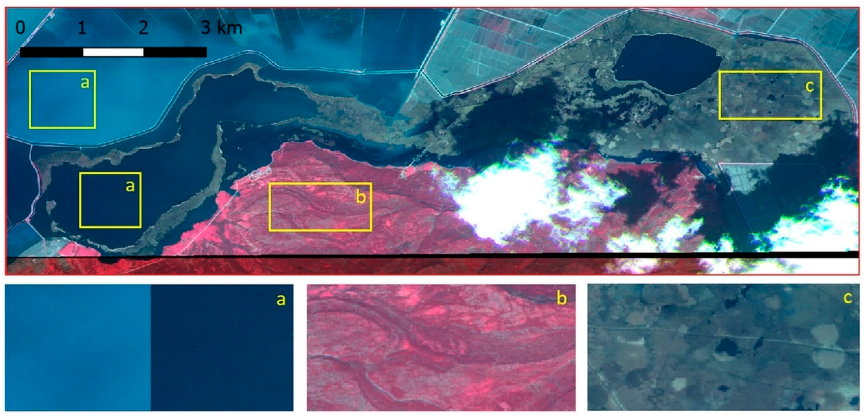
Figure 2.
High-resolution false-color (NIR (near infrared), green, blue) WorldView2 image (March 11, 2015) (© European Space Imaging/DigitalGlobe) for northern Greece/Turkey containing temporary flooded vegetation (TFV) (a), temporary open water (TOW) (b), and dry land (DL) (c).
Figure 2.
High-resolution false-color (NIR (near infrared), green, blue) WorldView2 image (March 11, 2015) (© European Space Imaging/DigitalGlobe) for northern Greece/Turkey containing temporary flooded vegetation (TFV) (a), temporary open water (TOW) (b), and dry land (DL) (c).

Figure 3.
High-resolution false-color (NIR, green, blue) RapidEye image (April 04, 2015). (© Planet Labs Inc.) for southern Greece/Turkey containing TOW (a), DL (b), and TFV (c).
Figure 3.
High-resolution false-color (NIR, green, blue) RapidEye image (April 04, 2015). (© Planet Labs Inc.) for southern Greece/Turkey containing TOW (a), DL (b), and TFV (c).

Figure 4.
Overview map with the location of the study area (red rectangle) in China (a), study area in China (b). The red rectangle represents the reference mask extent (c), which was derived from S-2 data (June 27, 2017).
Figure 4.
Overview map with the location of the study area (red rectangle) in China (a), study area in China (b). The red rectangle represents the reference mask extent (c), which was derived from S-2 data (June 27, 2017).

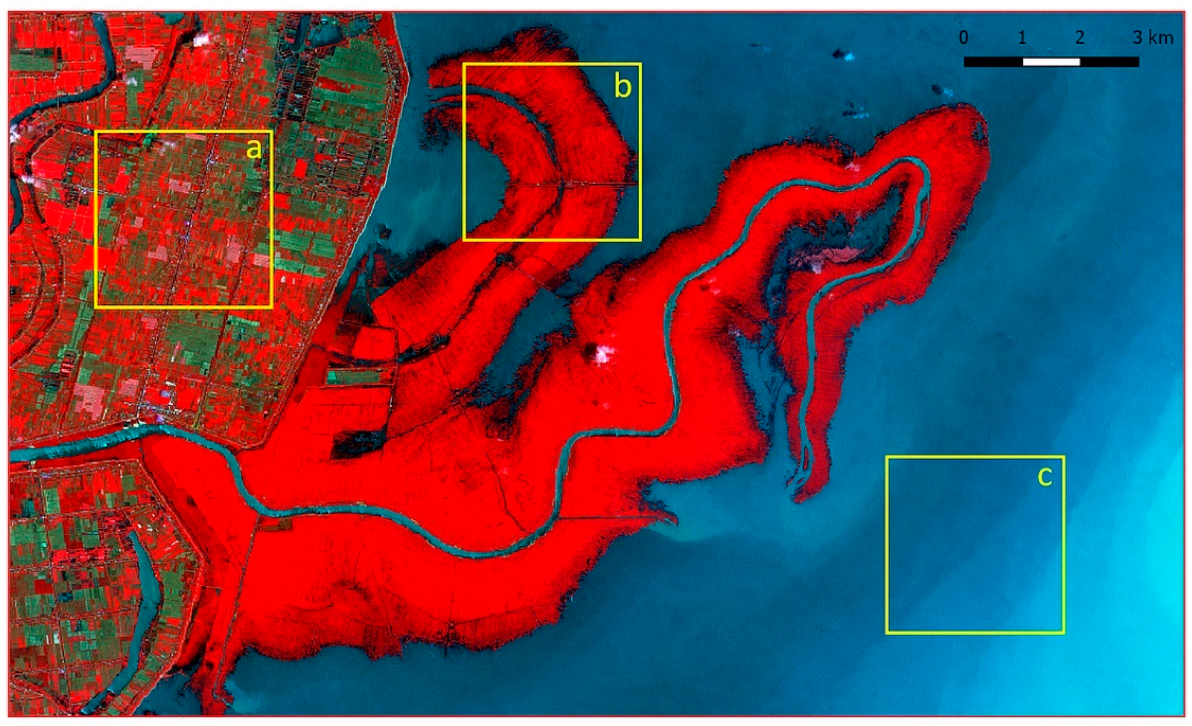
Figure 5.
High-resolution false-color (NIR, green, blue) Sentinel-2 image (June 27, 2017) for southern Greece/Turkey containing DL (a), TFV (b) and TOW (c).
Figure 5.
High-resolution false-color (NIR, green, blue) Sentinel-2 image (June 27, 2017) for southern Greece/Turkey containing DL (a), TFV (b) and TOW (c).

Figure 6.
Multitemporal behavior of the backscatter intensity for TOW areas for VV (decibel (dB)), VH (dB), VV/VH (linear scale), and Normalized Difference Vegetation Index (NDVI) values in northern Greece/Turkey. The blue bars mark the analyzed date at the flood event.
Figure 6.
Multitemporal behavior of the backscatter intensity for TOW areas for VV (decibel (dB)), VH (dB), VV/VH (linear scale), and Normalized Difference Vegetation Index (NDVI) values in northern Greece/Turkey. The blue bars mark the analyzed date at the flood event.

Figure 7.
Multitemporal behavior of the backscatter intensity for TFV areas for VV (dB), VH (dB), VV/VH (linear scale), and NDVI values in southern Greece/Turkey. The blue bars mark the analyzed date at the flood event.
Figure 7.
Multitemporal behavior of the backscatter intensity for TFV areas for VV (dB), VH (dB), VV/VH (linear scale), and NDVI values in southern Greece/Turkey. The blue bars mark the analyzed date at the flood event.

Figure 8.
Multitemporal behavior of the backscatter intensity for TFV areas for VV (dB), VH (dB), VV/VH (linear scale), and NDVI values in northern Greece/Turkey. The blue bars mark the analyzed date at the flood event.
Figure 8.
Multitemporal behavior of the backscatter intensity for TFV areas for VV (dB), VH (dB), VV/VH (linear scale), and NDVI values in northern Greece/Turkey. The blue bars mark the analyzed date at the flood event.

Figure 9.
Multitemporal behavior of the backscatter intensity for TFV areas for VV (dB), VH (dB), VV/VH (linear scale), and NDVI values in China. The blue bars mark the analyzed date at the flood event.
Figure 9.
Multitemporal behavior of the backscatter intensity for TFV areas for VV (dB), VH (dB), VV/VH (linear scale), and NDVI values in China. The blue bars mark the analyzed date at the flood event.

Figure 10.
Pixel-based classification result (a), object-based classification result (b) for the study area in southern Greece/Turkey.
Figure 10.
Pixel-based classification result (a), object-based classification result (b) for the study area in southern Greece/Turkey.

Figure 11.
Pixel-based classification result (a) and object-based classification result (b) for the study area in northern Greece/Turkey.
Figure 11.
Pixel-based classification result (a) and object-based classification result (b) for the study area in northern Greece/Turkey.

Figure 12.
Pixel-based classification result (a), object-based classification result (b) and validation mask (c) for the study area in China.
Figure 12.
Pixel-based classification result (a), object-based classification result (b) and validation mask (c) for the study area in China.

Figure 13.
Comparison of pixel-based time series features as a function of mean value and coefficient of variation. The statistical values (mean value and coefficient of variance) were calculated on the basis of the PA and UA accuracy values.
Figure 13.
Comparison of pixel-based time series features as a function of mean value and coefficient of variation. The statistical values (mean value and coefficient of variance) were calculated on the basis of the PA and UA accuracy values.

Figure 14.
Comparison of object-based time series features as a function of mean value and coefficient of variation. The statistical values (mean value and coefficient of variance) were calculated on the basis of the PA and UA accuracy values.
Figure 14.
Comparison of object-based time series features as a function of mean value and coefficient of variation. The statistical values (mean value and coefficient of variance) were calculated on the basis of the PA and UA accuracy values.


Table 1.
Acquisition dates of the Sentinel (S-1) satellite data used for Greece/Turkey. The scenes acquired on March 12, 2015 and April 5, 2015 (highlighted with blue background) were used as flood event images for two different parts (northern and southern) of the Greece/Turkey study area.
Table 1.
Acquisition dates of the Sentinel (S-1) satellite data used for Greece/Turkey. The scenes acquired on March 12, 2015 and April 5, 2015 (highlighted with blue background) were used as flood event images for two different parts (northern and southern) of the Greece/Turkey study area.
| No | Date | No | Date | No | Date | No | Date |
|---|---|---|---|---|---|---|---|
| 1 | October 19, 2014 | 16 | June 16, 2015 | 31 | January 6, 2016 | 46 | July 16, 2016 |
| 2 | October 31, 2014 | 17 | June 28, 2015 | 32 | January 18, 2016 | 47 | July 28,2016 |
| 3 | November 24, 2014 | 18 | July 10, 2015 | 33 | January 30, 2016 | 48 | August 9, 2016 |
| 4 | December 6, 2014 | 19 | July 22, 2015 | 34 | February 11, 2016 | 49 | August 21, 2016 |
| 5 | December 18, 2014 | 20 | August 15, 2015 | 35 | February 23, 2016 | 50 | September 2, 2016 |
| 6 | December 30, 2014 | 21 | August 27, 2015 | 36 | March 6, 2016 | 51 | September 14, 2016 |
| 7 | January 11, 2015 | 22 | September 8, 2015 | 37 | March 18, 2016 | 52 | September 26, 2016 |
| 8 | February 4, 2015 | 23 | September 20, 2015 | 38 | March 30, 2016 | 53 | October 2, 2016 |
| 9 | February 16, 2015 | 24 | October 2, 2015 | 39 | April 11, 2016 | 54 | October 14, 2016 |
| 10 | March 12, 2015 | 25 | October 14, 2015 | 40 | April 23, 2016 | 55 | October 26, 2016 |
| 11 | March 24, 2015 | 26 | October 26, 2015 | 41 | May 5, 2016 | 56 | November 7, 2016 |
| 12 | April 5, 2015 | 27 | November 19, 2015 | 42 | May 17, 2016 | 57 | November 19, 2016 |
| 13 | April 17, 2015 | 28 | December 1, 2015 | 43 | May 29, 2016 | 58 | December 1, 2016 |
| 14 | May 11, 2015 | 29 | December 13, 2015 | 44 | June 10,2016 | 59 | December 13, 2016 |
| 15 | June 4, 2015 | 30 | December 25, 2015 | 45 | July 4, 2016 | 60 | December 25, 2016 |
Table 2.
Acquisitions dates of the S-1 satellite data used for China. The scene acquired on June 28, 2017 (highlighted with blue background) was used within this study as a flood event image.
Table 2.
Acquisitions dates of the S-1 satellite data used for China. The scene acquired on June 28, 2017 (highlighted with blue background) was used within this study as a flood event image.
| No | Date | No | Date | No | Date | No | Date |
|---|---|---|---|---|---|---|---|
| 1 | October 19, 2016 | 11 | February 16, 2017 | 21 | July 10, 2017 | 31 | November 19, 2017 |
| 2 | October 31, 2016 | 12 | February 28, 2017 | 22 | July 22, 2017 | 32 | December 1, 2017 |
| 3 | November 12, 2016 | 13 | March 12, 2017 | 23 | August 3, 2017 | 33 | December 13, 2017 |
| 4 | November 24, 2016 | 14 | March 24, 2017 | 24 | August 15, 2017 | 34 | December 25, 2017 |
| 5 | December 6, 2016 | 15 | April 5, 2017 | 25 | August 27, 2017 | 35 | January 6, 2018 |
| 6 | December 18, 2016 | 16 | April 17, 2017 | 26 | September 8, 2017 | 36 | January 30, 2018 |
| 7 | December 30, 2016 | 17 | April 29, 2017 | 27 | October 2, 2017 | 37 | February 11, 2018 |
| 8 | January 11, 2017 | 18 | June 11, 2017 | 28 | October 14, 2017 | 38 | February 23, 2018 |
| 9 | January 23, 2017 | 19 | June 4, 2017 | 29 | October 26, 2017 | ||
| 10 | February 4, 2017 | 20 | June 28, 2017 | 30 | November 7, 2017 |
Table 3.
Characteristics of the S-1 data used.
| Sensor Properties | Values |
|---|---|
| Wavelength Mode | Interferometric Wide Swath (IW) |
| Polarization | VV − VH |
| Frequency | C-band (GHz) |
| Resolution | 20 × 22 m (az. × gr. range) |
| Pixel spacing | 10 × 10 m (az. × gr. range) |
| Inc. angle | 30.5°–46.3° |
| Orbit | Ascending |
| Product-level | Level-1 (Ground Range Detected High Resolution (GRDH)) |
Table 4.
Random forest importance analysis of the time series features for TOW and individual study areas. The rows highlighted in blue represent the time series features with the highest contribution (importance).
Table 4.
Random forest importance analysis of the time series features for TOW and individual study areas. The rows highlighted in blue represent the time series features with the highest contribution (importance).
| Southern Greece/Turkey (%) | Northern Greece/Turkey (%) | China (%) | |
|---|---|---|---|
| Z-Score VV | 35.64 | 29.26 | 31.35 |
| Z-Score VH | 15.51 | 23.07 | 24.61 |
| Z-Score VV + VH | 39.44 | 35.3 | 33.37 |
| Z-Score VV – VH | 5.91 | 7.33 | 3.87 |
| Z-Score VV/VH | 3.51 | 5.08 | 6.81 |
Table 5.
Random forest importance analysis of the time series features for TFV and individual study areas. The rows highlighted in green represent the time series features with the highest contribution (importance).
Table 5.
Random forest importance analysis of the time series features for TFV and individual study areas. The rows highlighted in green represent the time series features with the highest contribution (importance).
| Southern Greece/Turkey (%) | Northern Greece/Turkey (%) | China (%) | |
|---|---|---|---|
| Z-Score VV | 32.61 | 28.39 | 33.21 |
| Z-Score VH | 2.79 | 11.30 | 17.32 |
| Z-Score VV + VH | 18.66 | 21.53 | 33.84 |
| Z-Score VV – VH | 41.57 | 16.37 | 8.56 |
| Z-Score VV/VH | 4.38 | 22.41 | 7.10 |
Table 6.
Accuracy assessment for the pixel- and object-based classification for the individual study areas. Overall accuracy (OA) in %, Producer accuracy (PA) in %, User accuracy (UA) in %, and Kappa index (K).
Table 6.
Accuracy assessment for the pixel- and object-based classification for the individual study areas. Overall accuracy (OA) in %, Producer accuracy (PA) in %, User accuracy (UA) in %, and Kappa index (K).
| Southern Greece/Turkey (%) | Northern Greece/Turkey (%) | China (%) | ||||
|---|---|---|---|---|---|---|
| Pixel-based | Object-based | Pixel-based | Object-based | Pixel-based | Object-based | |
| DL—UA | 76.64 | 77.62 | 56.65 | 53.25 | 85.26 | 87.66 |
| TOW—UA | 86.53 | 86.87 | 97.58 | 98.23 | 79.73 | 85.65 |
| TFV—UA | 90.37 | 92.17 | 76.83 | 73.86 | 78.28 | 83.01 |
| DL—PA | 77.86 | 79.61 | 91.67 | 96.60 | 69.89 | 78.95 |
| TOW—PA | 85.94 | 86.38 | 91.02 | 91.67 | 90.47 | 91.14 |
| TFV—PA | 89.52 | 90.09 | 28.18 | 6.32 | 90.09 | 91.23 |
| OA | 84.26 | 85.17 | 81.47 | 79.59 | 81.37 | 85.84 |
| Kappa | 0.76 | 0.78 | 0.66 | 0.63 | 0.71 | 0.78 |
Table 7.
The accuracy values PA and UA of the pixel-based classification for the individual study areas as a function of the five analyzed time series features. The relevant time series features for the individual study areas, which were identified by the Random Forest Algorithm (Section 3.1) and corresponding PA and UA values are highlighted in dark green. Optimum of statistical variables (mean value of UA / PA and coefficient of variables) for time series features is highlighted in light green.
| Z-Score VV | Z-Score VH | Z-Score VV + VH | Z-Score VV − VH | Z-Score VV/VH | ||||||
|---|---|---|---|---|---|---|---|---|---|---|
| UA | PA | UA | PA | UA | PA | UA | PA | UA | PA | |
| Namibia | 88.72 | 78.43 | 47.11 | 90.52 | 85.64 | 82.38 | 92.62 | 69.96 | 67.90 | 86.32 |
| China | 82.26 | 92.65 | 51.26 | 99.30 | 78.28 | 90.09 | 52.37 | 99.24 | 44.46 | 99.50 |
| North Greece | 76.83 | 28.18 | 50.34 | 0.81 | 65.85 | 3.26 | 37.10 | 4.71 | 68.58 | 56.72 |
| South Greece | 96.10 | 77.17 | 35.25 | 42.22 | 94.89 | 53.17 | 90.37 | 89.52 | 60.85 | 93.48 |
| Mean values of UA and PA | 77.54 | 52.10 | 69.18 | 65.74 | 72.23 | |||||
| Coefficient of variance | 0.22 | 0.41 | 0.36 | 0.47 | 0.18 | |||||
Table 8.
The accuracy values PA and UA of the object-based classification for the individual study areas as a function of the five analyzed time series features. The relevant time series features for the individual study areas, which were identified by the Random Forest Algorithm (Section 3.1) and corresponding PA and UA values are highlighted in dark green. Optimum of statistical variables (mean value of UA / PA and coefficient of variables) for time series features is highlighted in light green.
| Z-Score VV | Z-Score VH | Z-Score VV + VH | Z-Score VV − VH | Z-Score VV/VH | ||||||
|---|---|---|---|---|---|---|---|---|---|---|
| UA | PA | UA | PA | UA | PA | UA | PA | UA | PA | |
| Namibia | 84.05 | 80.71 | 49.26 | 17.47 | 84.37 | 5.99 | 54.93 | 89.29 | 76.1 | 91.2 |
| China | 82.38 | 92.65 | 62.51 | 92.46 | 83.01 | 91.23 | 66.68 | 97.06 | 42.86 | 97.86 |
| North Greece | 73.86 | 6.32 | 50.35 | 0.82 | 65.99 | 3.29 | 48.61 | 2.92 | 68.75 | 57.22 |
| South Greece | 97.05 | 87.81 | 26.90 | 31.64 | 98.52 | 75.19 | 92.17 | 90.09 | 65.20 | 92.74 |
| Mean values of UA and PA | 75.57 | 41.43 | 63.44 | 67.72 | 73.99 | |||||
| Coefficient of variance | 0.31 | 0.62 | 0.52 | 0.40 | 0.19 | |||||
© 2019 by the authors. Licensee MDPI, Basel, Switzerland. This article is an open access article distributed under the terms and conditions of the Creative Commons Attribution (CC BY) license (http://creativecommons.org/licenses/by/4.0/).
Share and Cite
MDPI and ACS Style
Tsyganskaya, V.; Martinis, S.; Marzahn, P. Flood Monitoring in Vegetated Areas Using Multitemporal Sentinel-1 Data: Impact of Time Series Features. Water 2019, 11, 1938. https://doi.org/10.3390/w11091938
AMA Style
Tsyganskaya V, Martinis S, Marzahn P. Flood Monitoring in Vegetated Areas Using Multitemporal Sentinel-1 Data: Impact of Time Series Features. Water. 2019; 11(9):1938. https://doi.org/10.3390/w11091938
Chicago/Turabian StyleTsyganskaya, Viktoriya, Sandro Martinis, and Philip Marzahn. 2019. "Flood Monitoring in Vegetated Areas Using Multitemporal Sentinel-1 Data: Impact of Time Series Features" Water 11, no. 9: 1938. https://doi.org/10.3390/w11091938
Note that from the first issue of 2016, this journal uses article numbers instead of page numbers. See further details here.