A Numerical Study of Fluid Flow in a Vertical Slot Fishway with the Smoothed Particle Hydrodynamics Method
by
 , , ,
, , ,
Gorazd Novak
1 ,
,
Angelantonio Tafuni
2,* ,
,
José M. Domínguez
3,
Matjaž Četina
1 and
Dušan Žagar
1,* 1
Faculty of Civil and Geodetic Engineering, University of Ljubljana, 1000 Ljubljana, Slovenia
2
School of Applied Engineering and Technology, New Jersey Institute of Technology, Newark, NJ 07103, USA
3
EPHYSLAB Environmental Physics Laboratory, University of Vigo, 32004 Ourense, Spain
*
Authors to whom correspondence should be addressed.
Water 2019, 11(9), 1928; https://doi.org/10.3390/w11091928
Submission received: 27 July 2019
/
Revised: 9 September 2019
/
Accepted: 10 September 2019
/
Published: 15 September 2019
(This article belongs to the Section Hydraulics and Hydrodynamics)
Abstract
:Fishways have a great ecological importance as they help mitigate the interruptions of fish migration routes. In the present work, the novel DualSPHysics v4.4 solver, based on the smoothed particle hydrodynamics method (SPH), has been applied to perform three-dimensional (3-D) simulations of water flow in a vertical slot fishway (VSF). The model has been successfully calibrated against published field data of flow velocities that were measured with acoustic Doppler velocity probes. A state-of-the-art algorithm for the treatment of open boundary conditions using buffer layers has been applied to accurately reproduce discharges, water elevations, and average velocity profiles (longitudinal and transverse velocities) within the observed pool of the VSF. Results herein indicate that DualSPHysics can be an accurate tool for modeling turbulent subcritical free surface flows similar to those that occur in VSF. A novel relation between the number of fluid particles and the artificial viscosity coefficient has been formulated with a simple logarithmic fit.
1. Introduction
Fishways (or fish passes) have a great ecological importance as they help mitigate the interruptions of fish migration routes. These interruptions are usually caused by dams of hydropower plants (HPP), and fishways are often the only way to make it possible for aquatic fauna to pass obstacles that block their up-river journey [1]. This mitigation can only be effective if a fishway functions properly, which requires adequate flow characteristics related to optimal position, fish pass entrance, attraction flow, exit conditions, discharge, lengths, slopes, resting pools, design of the bottom, operating times, maintenance, and measures to avoid disturbances and to protect the fish pass [1].
Tan et al., (2018) [2] showed that hydraulic stimulus variables playing an important role in the functionality of a fishway include turbulent kinetic energy, velocity, and strain rate. Work therein also infer that fish could be responding to mesoscale hydraulic features such as velocity gradients, circulation, and vorticity in flow. These were investigated by Crowder and Diplas, (2006) [3], and Shen and Diplas, (2008) [4], who used spatial hydraulic metrics of vorticity and circulation.
Fish passes are generally divided into three groups: Denil fishways, pool and weir fishways, and vertical slot fishways (VSFs) [1,5]. This paper focuses on the VSFs, which are more often adopted for upstream passage of fish in river obstructions. A VSF is (usually) a rectangular channel with sloping floor that is divided into several pools. Water flows from one pool to the next through a vertical slot, at which a jet is formed. The jet creates recirculation regions, while the energy of the jet is dissipated by mixing and circulation in the pool. There are various methods and guidelines to design a VSF, whose main aim is to effectively dissipate the energy of the inlet jet and to create flow conditions in the pool that enable the fish to ascend without undue stress, i.e., (1) to simply pass via the slot at their preferred water depth, and (2) to rest in the recirculation regions, where low levels of energy dissipation constitute favorable resting areas [6]. Flow in VSFs is considered favorable for three reasons: (1) in the transition region between consecutive pools, fish have the option to select the depth of passage, since the opening is across the depth; (2) in each pool, there is generally a large resting region where the velocities are much lower than in the main jet, which can be very favorable when a high number of pools are needed to overcome the vertical gradient; (3) the main jet, where the maximum velocities are found, clearly identifies the upstream direction, which minimizes the chances of disorientation of fish along the route [7]. It should be noted that these features do not necessarily provide suitable flow conditions by themselves, since vortices can entrap the fish, as explained in Odeh et al., (2002) [8]. This means the flow pattern is of critical importance to the functionality of a VSF [1,5].
VSF have been the subject of numerous studies, including scale models, field measurements, and numerical models (e.g., Puertas et al., 2004 [9]; Tarrade et al., 2008 [10]; Chorda et al., 2010 [11]; Bombač et al., 2015 [12]; Marriner et al., 2016 [13]). Studies have shown that the structure of flow in VSF is mostly two-dimensional (2-D), with vertical component of the flow velocity being much lower than the horizontal ones, i.e., longitudinal and transverse. Despite the possible three-dimensional local velocity gradient in the slot zone, the flow in major areas of the pool is quasi two-dimensional (Wu et al., 1999 [14]; Liu et al., 2006 [15]). Recent studies employed various depth-averaged 2-D models (Cea et al., 2007 [16]; Bermúdez et al., 2010 [17]; Bombač et al., 2017 [18], and also several 3-D models (Masayuki et al., 2009 [19]; Ferrand et al., 2013 [20]; Duguay et al., (2017) [21]; Gisen et al., 2017 [22]; Umeda et al., 2017 [23]), which continue to be employed for VSF optimization (Li et al., 2019 [24] and Sanagiotto et al., 2019 [7]). Field measurements in Bombač et al., (2015) [12] that are used for calibration of the numerical model presented in this work confirm that the flow in the observed VSF is mostly 2-D, with the exception of flow in the vicinity of the slot. Furthermore, 3-D models have two important advantages compared to 2-D ones [6]: (1) they solve 3-D continuity and momentum equations, thus the assumption of hydrostatic pressure distribution is not required, (2) they employ a method that allows the unrestricted 3-D movement of the water surface. In contrast to most researchers, who use commercial computational fluid dynamics (CFD) codes, this paper presents an application of an open-source 3-D solver.
Mao (2018) [5] showed that despite the numerous studies, many existing fishways are still not functioning properly. This is probably due to the fact that most studies on fishway modeling lack animal experimentation and proper validation in a physical model—two recent exceptions being studies by Tan et al., (2018) [2] and Romão et al., (2018) [25]. Hence this field of research remains relevant, especially in light of the fact that compliance with the European Water Framework Directive and other water protection policies [26] requires restoration of river continuity through construction of efficient fishways [22,27]. This paper focuses on a well-functioning VSF that is located at the Arto–Blanca HPP on the river Sava in Slovenia. The functionality of this VSF has been confirmed in studies by Kolman et al., (2010) [28] and Ciuha et al., (2014) [29]. This VSF consists of two reaches: the upstream concrete reach with 24 vertical slots (i.e., VSF reach), and a much more natural-like downstream reach with meanders [12]. Field measurements by Bombač et al., (2015) [12] were performed in a VSF reach and were used as calibration data for the presented 3-D numerical model, based on the Smoothed particle hydrodynamics (SPH) method. SPH allows the computation of complex hydrodynamic problems. Because the fluid is discretized into particles, it is especially suitable for simulating interface flows, strong nonlinearities and fluid-structure interactions in the presence of moving objects (Tafuni et al., 2015 [30]; Canelas et al., 2017 [31]; Sun et al., 2018 [32]; Gonzáles-Cao et al., 2019 [33]), and can thus be applied to real life engineering problems in the industry or in the field of ecological engineering. Meshless approach of the SPH requires considerable processing power [34], but with the recent advances in graphics processing units (GPU) and related programming architectures (CUDA), and general-purpose GPU (GPGPU), the by-pass to this limitation is quickly becoming more affordable [35,36]. In contrast to other types of numerical models, SPH was applied to fish passes only in a few studies: Marivela and López (2009) [37] used a 3-D SPH model to optimize the hydraulic design of a VSF, focusing on the slot region and patterns of lateral recirculation. Ferrand et al., (2013) [20] repeated the simulations presented by Violeau et al., (2008) [38] and applied a 2-D model of a schematic fish pass to compare SPH with k- model and an Eulerian finite volume method; Gomes and Nascimento (2018) [39] applied the DualSPHysics code with periodic boundary conditions to model a fishway with trapezoidal cross sections. In this paper we are presenting the results obtained by the novel DualSPHysics v4.4 solver, and demonstrating its suitability for solving VSF related problems. The study has two main goals. First, to show that the SPH method can simulate free surface turbulent subcritical flow in a VSF accurately. The second goal is to investigate how the variation of the main execution parameters affects the resulting discharges and velocity fields, thus providing calibration guidelines for future studies. The paper focuses on the most important parameters, i.e., those related to spatial resolution (given by the initial interparticle distance) and viscosity (artificial viscosity coefficient; laminar viscosity and sub-particle scale (SPS) turbulence). Although flow conditions in this study are mostly 2-D, the use of a 3-D SPH model is found appropriate for several reasons: (1) the flow has a vertical component of velocity in the region of the jet. This component is small, but it does exist, making 3-D modeling the obvious choice. (2) Available field data is 3-D. Therefore 3-D simulations seem the most consistent choice for calibration. (3) With a relatively simple velocity field, the effects of various execution parameters can be more readily investigated and made available for future SPH studies. (4) By using a 3-D model, results herein are easily compared with those in Sanagiotto et al., (2019) [7], where data from another 3-D model is calibrated against the same 3-D field data [12,18] used for comparison in this work. Thus, a useful comparison between the two 3-D models is possible. (6) Finally, many SPH applications are 3-D, so it is reasonable to use a 3-D model when also trying to provide useful insights about the functionality of a SPH code.
2. SPH Formalism
The simulations presented in this paper were performed using DualSPHysics software [40], which is an established open-source parallel computational fluid dynamics (CFD) solver based on Smoothed particle hydrodynamics, a Lagrangian meshless method. SPH discretizes a continuum using a set of material points, called particles. The discretized Navier–Stokes equations are locally integrated at the location of each particle, according to the physical properties of surrounding particles. The set of neighboring particles is determined by a distance-based function, either circular (2-D) or spherical (3-D), with an associated characteristic length or smoothing length, denoted as h. At each time step, new physical quantities are calculated for each particle, which then move according to these updated values [40]. The effect the neighboring particles have on an individual particle, a, is weighted depending on their distance r from particle a, using a kernel function, W, and the smoothing length. The kernel is expressed as a function of the non-dimensional distance between particles, given as , where r is the distance between a certain particle a and a neighboring particle. Kernel functions can have different shapes and the choice of this function influences the performance of a SPH model quite significantly. The most commonly used kernel functions in SPH are the cubic [41] and quintic [42] kernels. Kernels have a so-called influence domain, which defines the area surrounding particle a within which neighboring particles influence particle a. In this work, a quintic kernel is applied, defined as:
where when dealing with 3-D simulations [43]. The smoothing length h is set equal to , with being the initial interparticle spacing. The influence domain adopted in the DualSPHysics code has a radius of , meaning that interactions between particles are neglected for distances between particles beyond , i.e., for .
2.1. Governing Equations
Like in other fluid dynamics models, the governing equations in SPH are Navier–Stokes equations, i.e., continuity equation (expressing the conservation of mass) and momentum equation (expressing the conservation of momentum), together with an equation of state which generally relates density , temperature T, salinity s, and pressure p. The general form of continuity equation is:
where , is the divergence operator, is the velocity vector, and is the fluid density. In SPH formulation, the continuity equation is discretized as:
where N is the total number of particles inside the kernel domain centered at target particle a, and are the mass and density of the interpolating particle b, and the notation = . For the momentum equation, a differential equation is given by the Navier–Stokes equations in vector form:
where ∇ (·) is the gradient operator, p is the pressure, is gravity, and is the deviatoric component of the total stress tensor. In its SPH formulation, the momentum equation is expressed as:
2.2. Viscosity Treatment and other Numerical Dissipation
For the treatment of the viscous term in Equation (5), the artificial viscosity model proposed by [43] is employed:
where , , and is the average numerical speed of sound between particles a and b. The primary purpose of this diffusion term is to deal with the instabilities that arise when using standard SPH algorithms to simulate liquid behavior and to handle its inability to capture shock waves. Based on experiments in a wave flume, Altomare et al., (2015) [44] proposed a reference value of for wave propagation and induced loading onto coastal structures, but they point out that should be tuned for every specific problem, and should in general be kept as small as possible to avoid numerical instabilities without leading to over-diffusive behavior.
Following the work of Monaghan (1994) [45], the fluid in the SPH formalism defined in DualSPHysics is treated as weakly compressible, and an equation of state is used to determine fluid pressure based on particle density, as follows:
where the polytropic constant is set to for water, kg m is the fluid reference density, , and is an artificial speed of sound at the reference density. The weak compressibility of the fluid allows the lowering of the speed of sound artificially to much smaller values than the physical speed of sound. This means that the value of time step at any moment can be maintained at a reasonable value. Typically, the speed of sound in Weakly Compressible SPH (WCSPH) is chosen to be at least ten times the maximum fluid velocity. This ensures that the fluid behaves closely to an incompressible fluid while keeping density variations to within 1%, see [30,40] for more details.
DualSPHysics allows two different options for including the effects of dissipation, i.e., two separate viscosity treatments: (1) the artificial viscosity seen above, and (2) a laminar viscosity and sub-particle scale (SPS) turbulence model. The artificial viscosity scheme is the most commonly used due to its simplicity, though it does not have any turbulence model and its use is often limited to laminar flow. The latter notwithstanding, the use of the artificial viscosity formulation has also been observed in several cases involving non-laminar flows, see references in Section 3 for more details. The concept of the sub-particle scale (SPS) was first described by Gotoh et al., (2004) [46], and was introduced into weakly compressible SPH by Dalrymple and Rogers (2006) [47] using Favre averaging. The momentum conservation equation can be written as (subscripts and superscripts refer to particles a and b):
with
Here i and j represent coordinate directions, is the sub-particle stress tensor, is the turbulent eddy viscosity, k is the SPS turbulence kinetic energy per unit mass, is the Smagorinsky constant, = 0.0066, and , where is an element of the SPS strain tensor. We adopted the value of kinematic viscosity of m/s, which is the kinematic viscosity of water at ambient temperature.
The equation of state describes a very stiff relationship between the pressure and density fields, which can lead to high-frequency low-amplitude oscillations [48]. This effect is enhanced by the natural disorder of Lagrangian particles. In order to mitigate these pressure fluctuations, the delta-SPH correction formulated by Marrone et al., (2011) [49] is introduced, with a corrective term added to the continuity equation as follows:
where the coefficient is used to tune the intensity of the diffusion (inactive when ). A value of is recommended for most applications [40], and this number was thus used throughout the cases presented in this paper.
2.3. Time Stepping
Numerical integration can be performed with various schemes available in the literature. The DualSPHysics code includes two options, Verlet and Symplectic algorithms. The former scheme is computationally simpler, while the symplectic scheme is more numerically stable but computationally expensive. The Verlet scheme provides a low computational overhead because it does not require multiple calculations for each step, e.g., predictor and corrector. In cases where the Verlet scheme is used but it is found that numerical stability is an issue or the scheme is not able to capture the dynamics of the case suitably, the symplectic scheme is the better choice. Given its second order accuracy in time, the symplectic scheme is used in this work.
3. Code Features and Boundary Conditions
DualSPHysics is a CPU/GPU WCSPH code with pre- and post-processing tools capable of performing simulations with millions and up to billions of particles, using the GPU architecture targeted to real life engineering problems involving non-linear, fragmented and free surface flows [35,40,50,51]. In the present study, the latest code release v4.4 of DualSPHysics is employed. Contrarily to other recent applications of DualSPHysics, which successfully simulated problems such as liquid sloshing [52], flow past submarines [53] and planing hulls [54], waves-structure interaction [55,56], and other complex hydrodynamic problems, this paper focuses on the application of open boundary conditions to solve turbulent free surface subcritical flow in a vertical slot fishway. The DualSPHysics code allows the selection of a wide range of execution parameters. The main ones are time integration schemes (Verlet, symplectic), kernel functions (cubic spline, quintic), density diffusion (delta-SPH), and viscosity formulations (artificial viscosity, laminar viscosity, and SPS turbulence model). The package also includes a variety of post-processing tools (e.g., FlowTool, MeasureTool, PartVTK) that aid in the quantification of the flow variables (fluid velocities, accelerations, forces etc.) at selected locations within the domain, and prepare them for further visualization.
Prior to the 4.4 release, DualSPHysics did not include open boundary conditions, thus a periodic boundary condition formalism had to be used to simulate inflow and outflow conditions. For a similar case of VSF with the same basic geometry but including several pools, a model with an initial fluid object and periodic boundary conditions was successfully presented in Novak et al., (2019) [57]. The new release of DualSPHysics allows simulating several types of open boundary conditions (e.g., inlet and outlet conditions), and they can be set up in the following ways: time- and/or space-dependent velocity fields can be assigned at an open boundary directly by the user or via an external file. Alternatively, the velocity can also be extrapolated from ghost nodes placed in the fluid near the open boundary using a first order consistent procedure described in detail in Tafuni et al., (2018) [58]. Similarly, the density at an open boundary can be either predefined (fixed and hydrostatic options available) or varied according to information from the ghost nodes. Finally, a condition on the water elevation is also available at the open boundaries, where the water level can either be predefined (fixed and time-dependent options available) or retrieved from the fluid nearby using the ghost nodes. Using buffer regions prevents errors generated by the kernel truncation near the boundaries, and particles inside the buffer areas are created and/or deleted to prevent the formation of voids. Furthermore, time-varying free surface elevation in the buffer regions can be extrapolated or imposed with minimum reflection of numerical noise into the fluid. Thus, these open boundary conditions can be used to impose inflow/outflow boundary conditions according to the different physical quantities imposed and/or extrapolated from the flow field.
The other important boundary condition concerns the discretization of a fixed or moving solid boundary. In DualSPHysics, this is achieved using dynamic boundary particles [59]. Also called dynamic boundary conditions (DBC), these can be applied to arbitrary 2-D and 3-D shapes, and have provided good validation in many engineering problems [30,53,60]. However, the use of DBC is sometimes problematic, as they exert high repulsive forces on the fluid particles, causing a gap to form between the fluid and the solid [56]. In the present work, a correction is applied to the DBC in accordance with principles of the open boundary algorithm described in Tafuni et al., (2018) [58]. While the velocity of the dynamic boundary particles is set to zero, the density and pressure are retrieved from the fluid domain using mirrored ghost nodes.
4. Experimental and Numerical Set-Ups
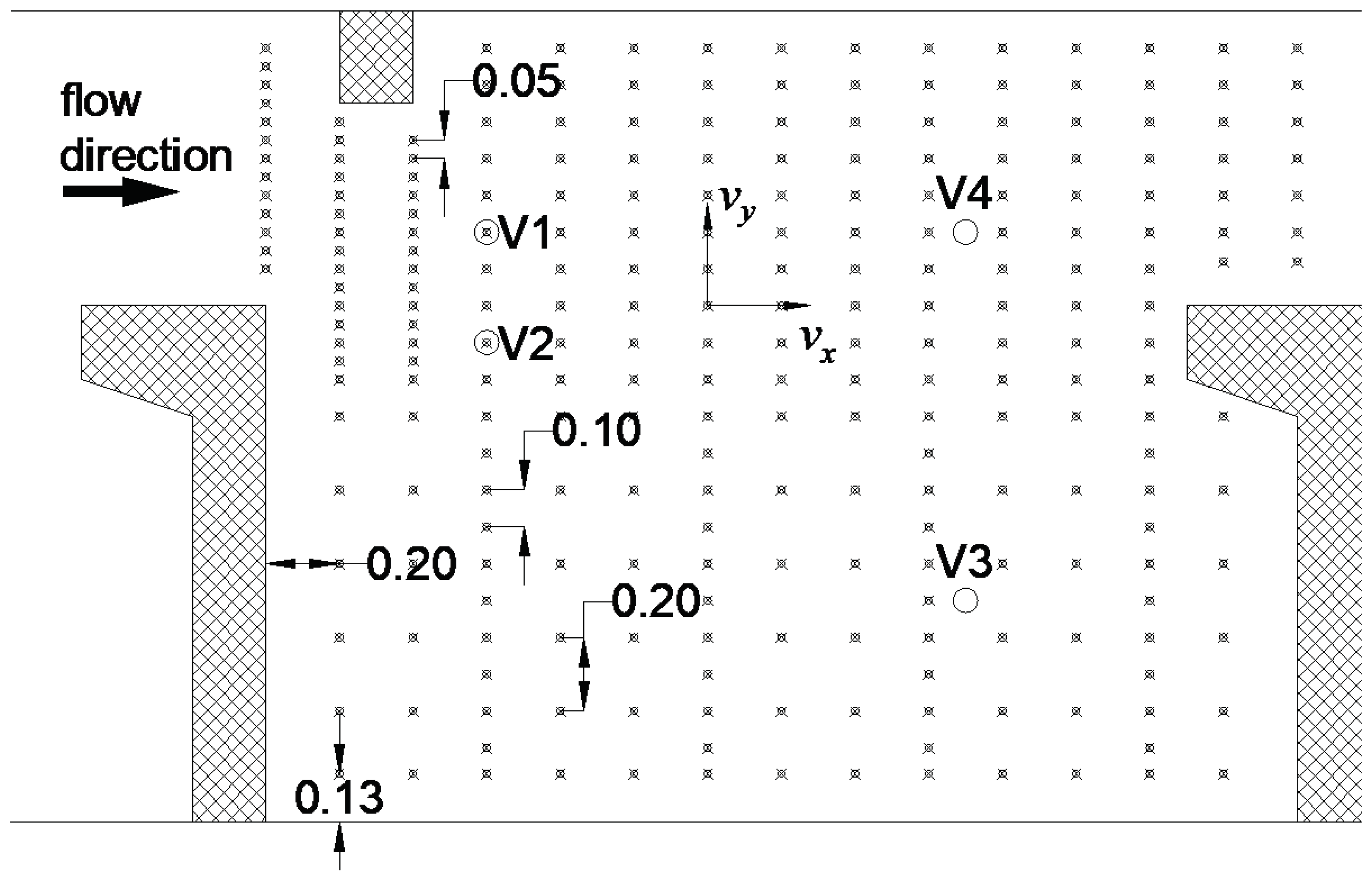
Simulations were calibrated against the existing field measurements described in Bombač et al., (2015) [12]. Measurements were obtained at the VSF situated at the Arto–Blanca HPP, which is in Slovenia (Europe), on river Sava. HPP Arto–Blanca is of the run-of-the-river and reservoir type, with three vertical generating units with a combined rated discharge of 500 m/s, five spillways and an average annual production output of 148 GWh. Field measurements were performed in steady-flow conditions, with a 1.0 m/s discharge and an average water depth of 1.3 m. The average water surface elevation was determined by leveling, and an acoustic Doppler velocimetry (ADV) probe was employed to measure velocity components at more than 250 points in the observed pool, as seen in Figure 1, taken directly from Bombač et al., (2015) [12]. The following parameters were measured: water surface elevation, bed elevation, and all three velocity components. Elevations were determined with leveling, while flow velocities were measured with a SonTek 3-D Micro-Acoustic Doppler Velocimeter (ADV). The probe was positioned with an adjustable traverse and caused negligible disturbance to the observed flow. The following user-defined settings were used: sampling frequency of 50 Hz, and measuring area of m/s. The suitability of the measurements was confirmed by an obtained signal correlation factor (with ) and signal-to-noise ratio (with ). Flow velocities were measured in a total of 254 points located 0.05 m to 0.20 m apart. Flow velocities were measured in two steps. First, the measurements were conducted at various depths in 4 verticals, shown in Figure 1 as V1 to V4. Results showed that the flow in the observed VSF was indeed two-dimensional, i.e., the vertical component of the velocity, w, was small while the horizontal components, u and v, remained practically constant for all . Additional measurements were performed in the first step to determine the time required for convergence of the measured values, i.e., the average of each velocity component and of turbulent kinetic energy. With the probe located at a different point in each of the mentioned 4 verticals (one point in each V1 to V4), measurements lasting up to 1222 s were then performed. Results showed that sufficient convergence () was achieved with measurements lasting 120 s. Measurements at vertical V3 were not presented, as this vertical location is near the center of the vortex, and consequently the measured average values are close to 0. Based on both findings from step one, velocity measurements were performed in all points shown at , with each measurement lasting 120 s.
Measured velocity fields indicated three regions of flow: the main flow through the slots, a larger recirculation in the pool behind the larger baffle, and a smaller recirculation immediately behind the smaller baffle. Comparison of both horizontal velocity components showed that measured longitudinal velocities were dominant over measured transverse velocity components, therefore we focused on the former when discussing the effects of various execution parameters in Section 5.
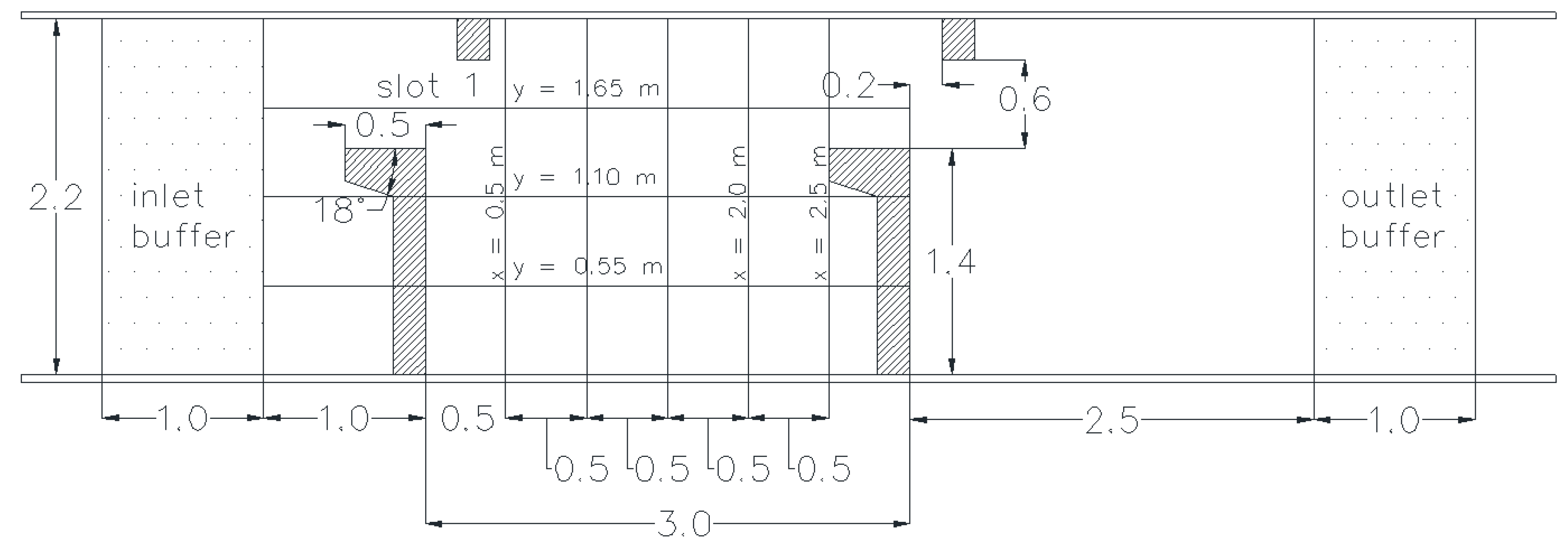
Preliminary simulations conducted in this work employed a geometry similar to the one described by Bombač et al., (2017) [18] and Novak et al., (2019) [57], i.e., an inlet section, nine pools, and an outlet section. Despite simulating several pools, both studies were focused only on a single pool in the middle of the VSF. The main results from the longer (nine pools) and the shorter (one pool) models showed only minor differences, indicating it was reasonable to use the shorter geometry. Thus, the VSF model described in this paper, consists of an inlet section, the observed pool, and an outlet section, as shown in Figure 2. Similar to the approach adopted for the simulation of open-channel flow in Tafuni et al., (2018) [58], a horizontal channel is used instead of an inclined one, the latter with a longitudinal slope of one degree. The baffles of the VSF have been tilted accordingly (counterclockwise by one degree) to allow for the correct simulation of the slope. Moreover, the gravity vector has been properly modified to account for the slope, i.e., a gravity vector m/s has been used in all simulations. This approach is adopted for a simpler implementation, in that the pre-processor used in this work generates SPH particles in the computational domain following a standard Cartesian grid. A sloped bed would cause not all SPH particles to lay on a perfectly flat plane, producing a stepped-like bed geometry that is nonphysical and as far from a flat bed as large is the value of the interparticle distance. The tilting of gravity vector provides proper driving forces and thus reproduces the physics of a sloped channel correctly. This has been done successfully in several other instances, such as for example the open-channel flow studied in [58]. Buffer regions representative of open boundary conditions are also easier to generate on such Cartesian mesh with a perfectly horizontal channel, rather than a sloped one. Other physical constants have been kept at their default values.
To set up the inlet and outlet of the VSF, variable velocity, extrapolated density, and fixed water elevation are adopted at the upstream and downstream ends of the VSF. This ensures a simulation of constant discharge, given as . Inlet and outlet velocities gradually increases from zero to 0.35 m/s in 6 s to avoid initial overflow, and then remains constant throughout the simulation. The density of buffer particles is extrapolated from the fluid adjacent to the buffer regions via the ghost nodes technique described earlier. The inlet and outlet buffers are set to include eight layers of particles, as recommended in Verbrugghe et al., (2019) [56] for open-channel flow. Water elevation H has been kept constant at 1.3 m. In all simulations, a ratio between the smoothing length and initial particle spacing has been used. A simulation time of 50 s has been chosen to allow the formation of the main recirculation in the observed pool. Outputs are saved every 0.2 s to capture the dynamics of the observed flow. Simulations with a particle spacing of 0.05 m resulted in approximately 240,000 initial particles, taking an average of 2.8 h of computational time on a single computer node with a NVIDIA GTX 1080 GPU.
5. Results and Discussion
The calibration of flow parameters is based on the following quantities: discharge Q in the slot, water elevation H along the pool, and profiles of longitudinal velocity u at locations m, 1.0 m, 1.5 m, 2.0 m and 2.5 m in the pool, as shown in Figure 2. Results from SPH simulations are evaluated primarily based on the obtained velocity profiles, as these were measured in the field with much greater accuracy than Q and H. Calibration includes several stages. Initial attention is dedicated to the effect of changing the particle resolution and choosing the right value of the viscosity coefficient, , as these are generally the most important parameters in the calibration of this SPH model. Additional simulations are also presented to address the use of different viscosity algorithms, i.e., using a Large Eddy Simulation (LES)-based model for turbulence. Results hereinafter present the difference between the two viscosity treatments. Optimal results are observed by applying the following combination of execution parameters: particle spacing m, time integration via the symplectic scheme, Wendland smoothing kernel, , .
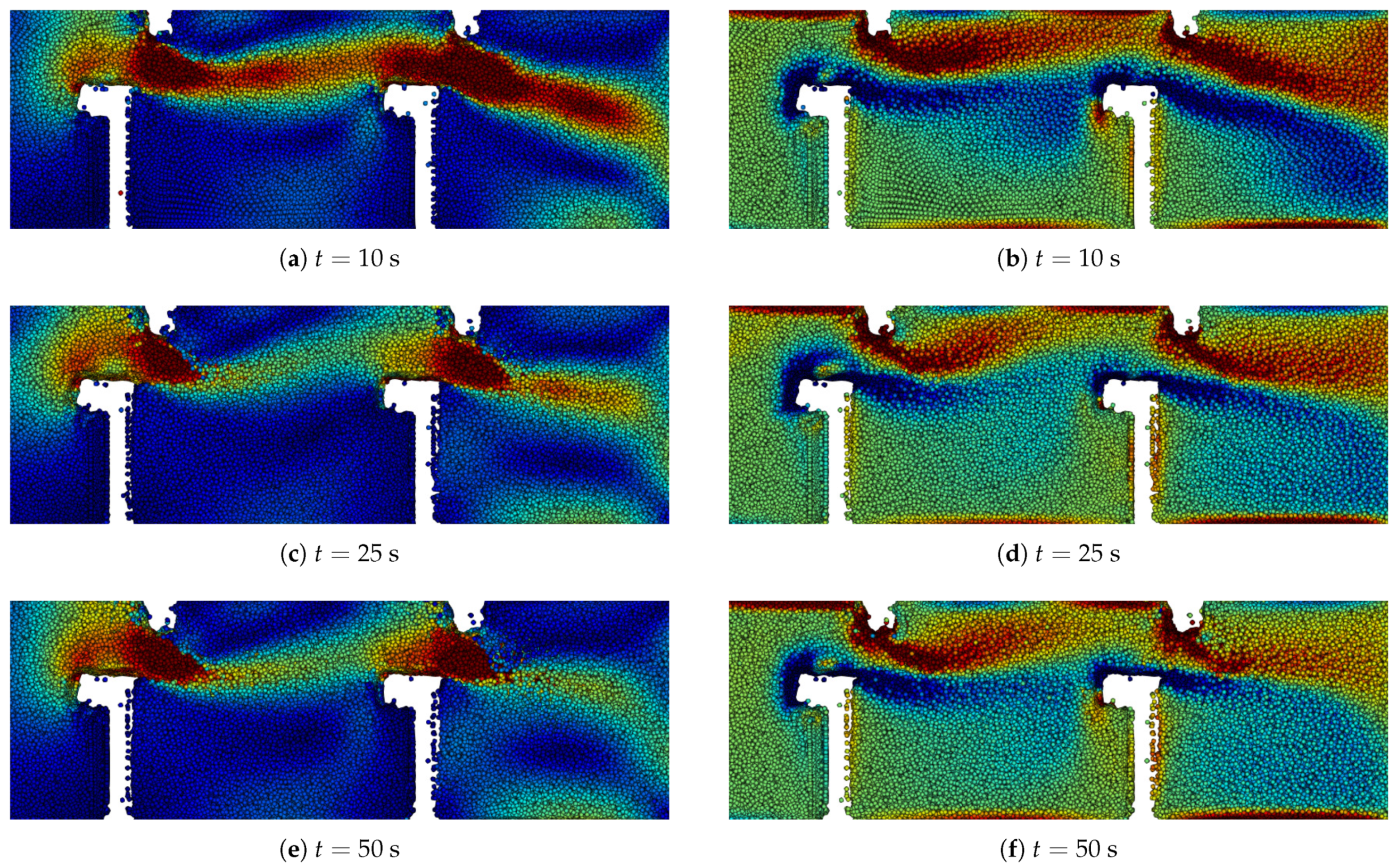
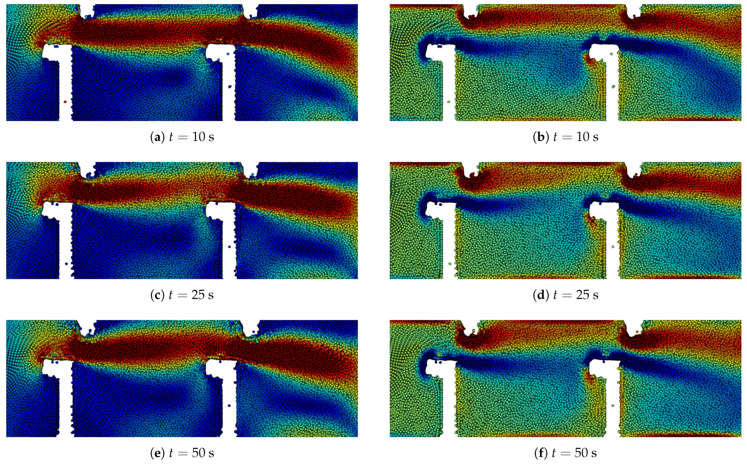
Figure 3 and Figure 4 present a top view of flow variables contours at different depths and different time instants. In particular, the left panels in both figures represent the flow velocity magnitude, ranging from 0 m/s (blue) to 1.5 m/s (red). The right panels symbolize vorticity in the vertical direction, ranging from –3.5 rad/s (blue) to 3.5 rad/s (red). The greatest velocities are attained in the slot region, where the water surface is more undulated than in the pool region, though flow conditions remain mostly 2-D. As can be seen by comparing velocities contours in Figure 3 and Figure 4 a higher velocity is observed in the slot regions at lower elevations than at the free surface. This also reflects in the vorticity contour maps, where larger rotational areas are observed at m than at m. The difference is attributed to the transfer of part of the flow kinetic energy to waves at the free surface. The results from the calibrated model are presented in the following sections, along with several variants highlighting the most significant findings.
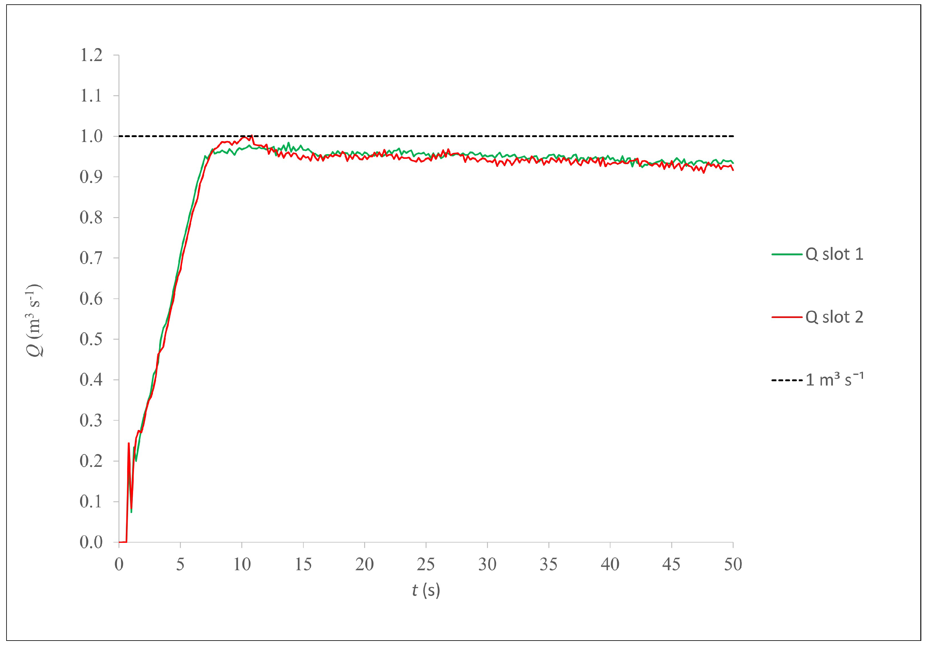
5.1. Discharge
The resulting discharge (i.e., the average Q over the last 10 s of the simulation) in both slots of the VSF is equal to 0.94 m/s, which is in good agreement with the measured value of 1.0 m/s. The time history of flow rate is shown in Figure 5. The gradual increase of Q from zero to a constant value in both slots can be noticed, complying with the boundary conditions at the inlet and outlet, where velocities are increased from zero to the constant value of 0.35 m/s in 6 s. Modeling the same VSF (existing geometry and field data for calibration) with an established commercial model, Sanagiotto et al., (2019) [7] achieved a better reproduction of m/s. This difference could be the result of a better formulation choice for boundary conditions and turbulence model. At the inlet, Sanagiotto et al., (2019) [7] used mass flow rates and applied a high turbulence intensity (10%) to specify the turbulence kinetic energy and the energy dissipation rate of the flow. In contrast, the discharge in DualSPHysics model was defined by imposing uniform velocity normal to the inlet cross section, without specifying turbulence characteristics. Prototype inlet conditions are similar to the ones used in our model, and field measurements do not necessarily support a definition of turbulence properties employed in [7].
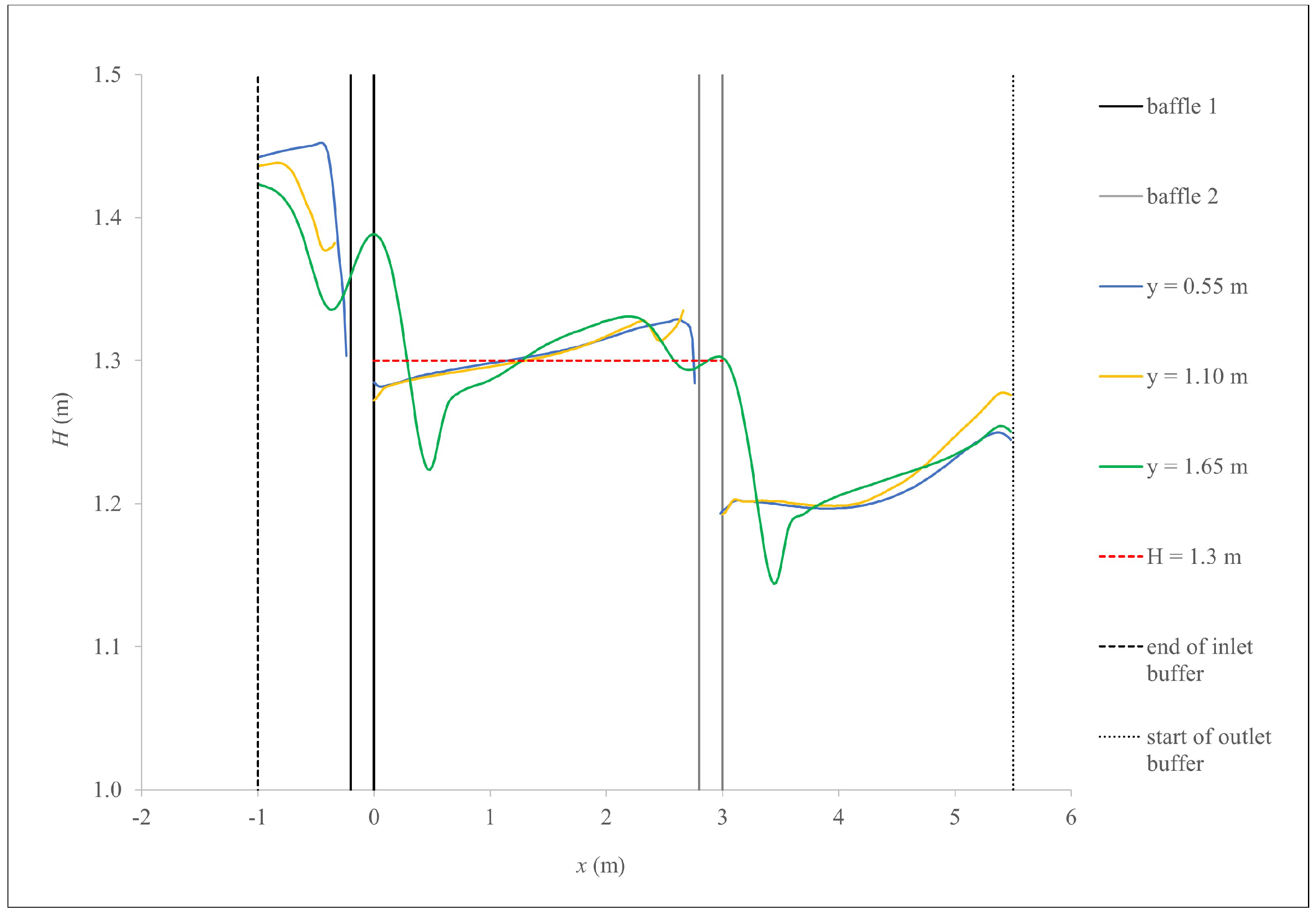
5.2. Water Elevation
The resulting water elevations (i.e., the average H over the last 10 s of the simulation) along the m, m, and m profiles (see Figure 2) in the observed pool are close to the measured average value of 1.3 m, as shown in Figure 6. Profiles indicate the water surface is more undulated in the slot regions (i.e., in the vicinity of the baffles in Figure 6), which is in accordance with field observations in Figure 7. The comparison is only qualitative, as water elevation was not measured to an accurate level of detail, hence no quantitative comparison is attempted. However, calculated water surface elevations are similar to those presented by Sanagiotto et al., (2019) [7]. In the region of the jet there is a trough in the water surface followed by a gradual increase of water depth. Closer to the right-side wall (i.e., within the observed pool) the longitudinal water elevation profile rises more gradually. This is expected because flow conditions there are less turbulent.
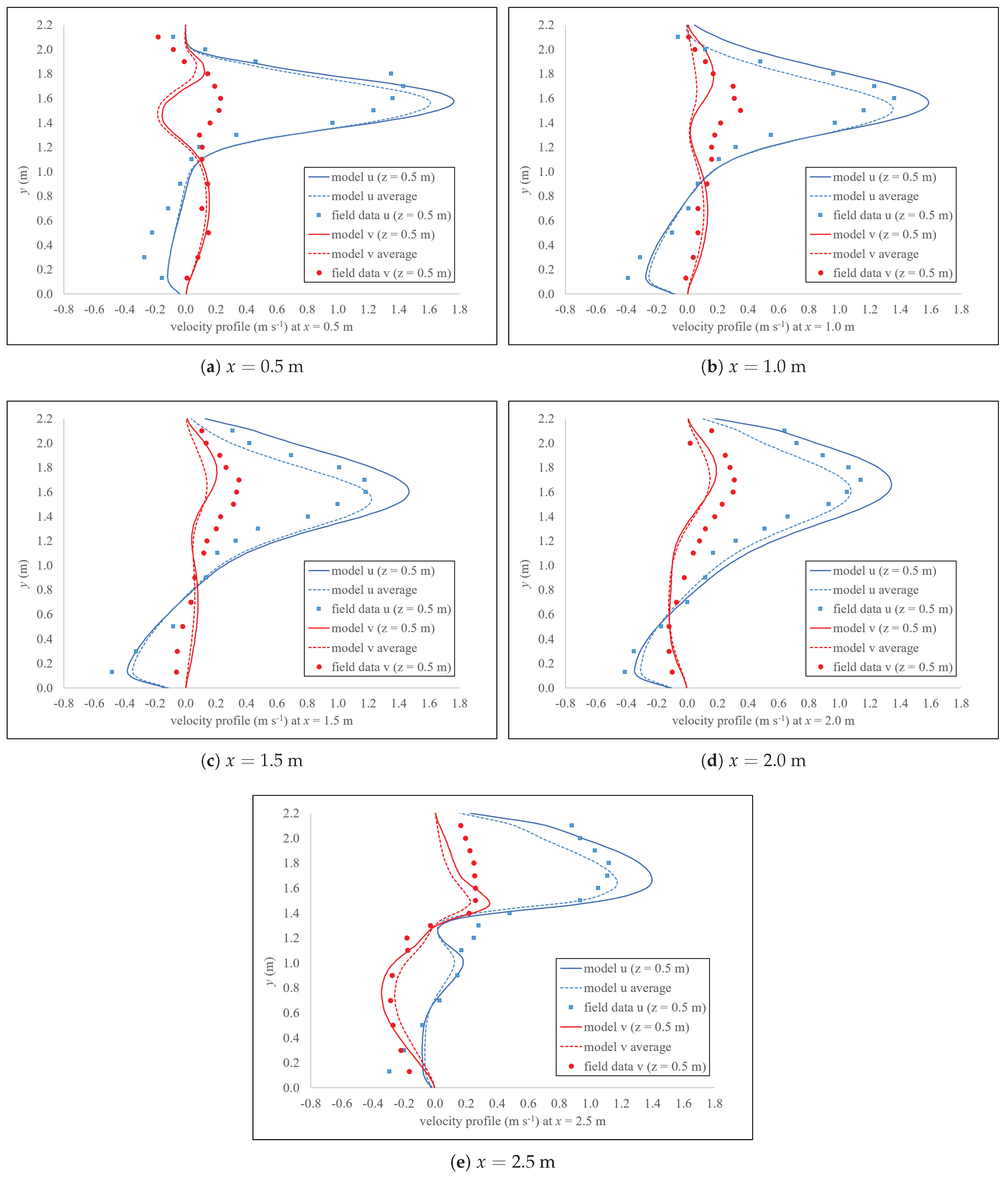
5.3. Velocity Profiles
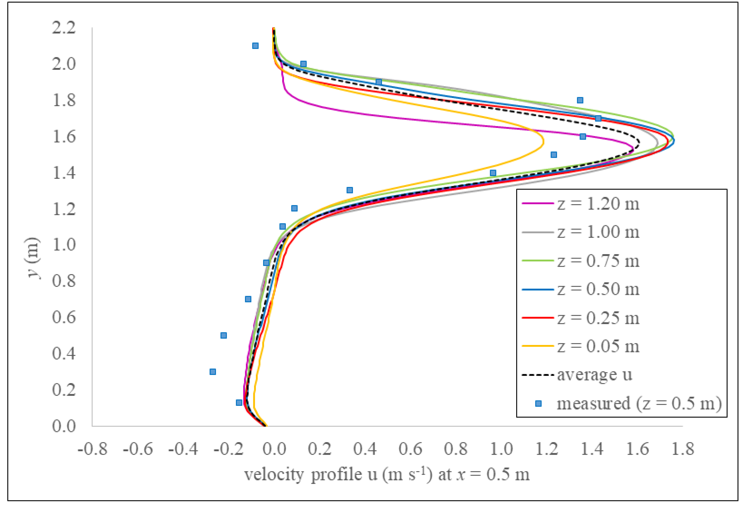
Velocity profiles are analyzed at cross sections x = 0.5 m, 1.0 m, 1.5 m, 2.0 m, and 2.5 m. At all cross sections, the velocities u and v are calculated at different depths, z, including m, 0.25 m, 0.50 m, 0.75 m, 1.00 m, and 1.20 m. The depth-averaged velocity (u or v) profile at a given cross section x is calculated from velocities (u or v) at six depths z at that location. These average velocity profiles are then compared to the values measured with ADV probe by Bombač et al., (2015) [12]. Figure 8a–e show velocity profiles calculated with the calibrated model. Therein, u and v profiles calculated with a calibrated DualSPHysics model agree qualitatively well with field data in [12]. Calculated v profiles run close to field data values (within 0.2 m/s difference), except in locations closer to the upstream slot, in the area of m to 1.0 m, and m to 1.8 m (Figure 8a,b). These velocities indicate that calculated jet coming out of the slot has partially (or locally) different direction than the measured one. However, values of v are close to zero (measured values are ranging from −0.3 m/s to 0.4 m/s in all cross sections) and much smaller than corresponding values u, so these differences do not play a significant role in relation to the overall velocity field in the observed pool.
Calculated u velocity profiles mostly run close to field data values (within 0.2 m/s difference). There are some discrepancies, which seem to be bigger near both walls, but it is worth mentioning that in the prototype VSF the velocities were in fact not measured exactly at the walls, so a detailed comparison is not possible. The use of uniform particle resolution also prevented the possibility of measuring velocity to the level of detail needed in the boundary layer, making it difficult to estimate the velocity in the close proximity of the wall. Close to the right-side wall, the model correctly shows the occurrence of backflow, but slightly underestimates velocity values of u, which are given in Table 1. Since field measurements were performed at m, profiles of u and v at m are shown in Figure 8 as well. It is evident that average profiles of u are closer to the measured values than calculated profiles at m. This can be expressed in terms of L-norm, given as a sum of distances between measured and calculated values in all measured points of a cross section, or
where n represents the number of points (16 in total) along an observed cross section. Values of L-norm for profiles of u shown in Figure 8 are 13.9 for u at m and 11.9 for the average u. In contrast, profiles of v at m are closer to the measured points than the average v, as indicated by an L-norm value of 7.6 and 9.0 for v at m and the average v, respectively. To further address the comparison between the measured and calculated values, we hereby report a two-tailed Wilcoxon signed-ranks test for paired samples with . Here represents the parameter used in the Wilcoxon test. Table 2 shows that significant differences are only noted for three cross sections, i.e., m, m, and m. These extend solely to v velocities, which have been shown to be far less important than u velocities when constructing the velocity vector.
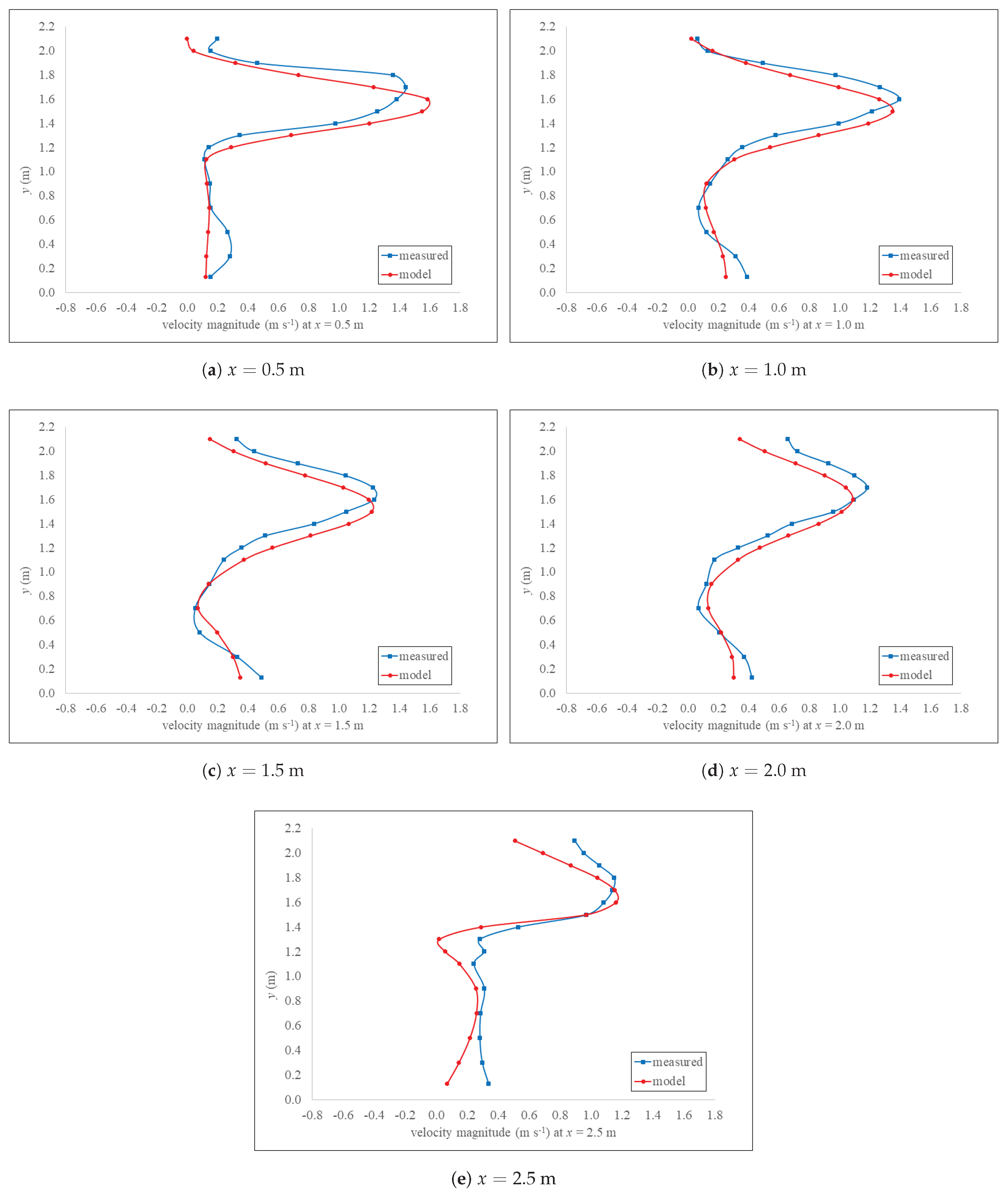
Some discrepancies can be observed in Figure 8. The most evident are those related to v profiles, especially in the slot region, i.e., m to m. However, vertical components of velocity are significantly smaller than horizontal components, thus the resulting velocity vectors given as are mostly determined by the value of the u component. The difference between measured and calculated values of v are thus significantly less important than the difference between measured and calculated values of u, which is substantially smaller. To emphasize this concept, Figure 9 depicts the magnitude V of measured and calculated flow velocities along the vertical direction, and at given x locations. The magnitude of the flow velocity vector is calculated as the length of the vector , namely . Clearly, the overall agreement between measured and calculated velocities becomes more evident. The largest differences between the measured and calculated values of v profiles occur close to the slot, i.e., at m, m to m, where the flow is significantly more complex than in the rest of the pool (3-D in the slot, 2-D elsewhere). The discrepancy could be because calculated values are an average of the last 10 s of the simulation, while the measured values at corresponding locations are an average of 120 s. For u profiles, however, the accuracy of the calculated average profiles is comparable to the results of other models of VSF at HPP Arto–Blanca, namely Bombač et al., (2015 and 2017) [12,18], where a depth-averaged 2-D model is employed, and Sanagiotto et al., (2019) [7], where a commercial 3-D model is applied. In the latter, a maximum longitudinal velocity of 1.62 m/s is shown at m. Our result at approximately the same location, i.e., at cross section m, is m/s, as seen by the maximum in the average profile of Figure 10. This shows that the two 3-D models agree well, giving approximately the same result in terms of velocity in the region of the main jet. From Figure 8 it is also evident that model does not perform well at some depths, since vertical distributions of SPH velocity are not as uniform as field measurements indicate. This can be better observed in Figure 10, showing calculated u profiles at various z for the most problematic locations, i.e., at the cross section m. Discrepancies are likely due to the boundary condition formulation used to discretize solid boundaries in DualSPHysics. This work represents the first application of dynamic boundary particles (with an active correction for the density) to the case of subcritical turbulent open-channel flow in a VSF, and as such, some inconsistencies have arisen. Dynamic boundary particles locally affect the velocities near the channel bed (see curve m in Figure 10), dissipating the flow kinetic energy at greater depths z, i.e., in the vicinity of the VSF bed.
Despite the discrepancies near solid boundaries (bed and both side walls), which seem to relate to the model’s inherent limitations when simulating solid walls (boundary correction, effective dimension of the slot), the overall performance of the DualSPHysics model remains comparable to numerical models employed in previous studies.
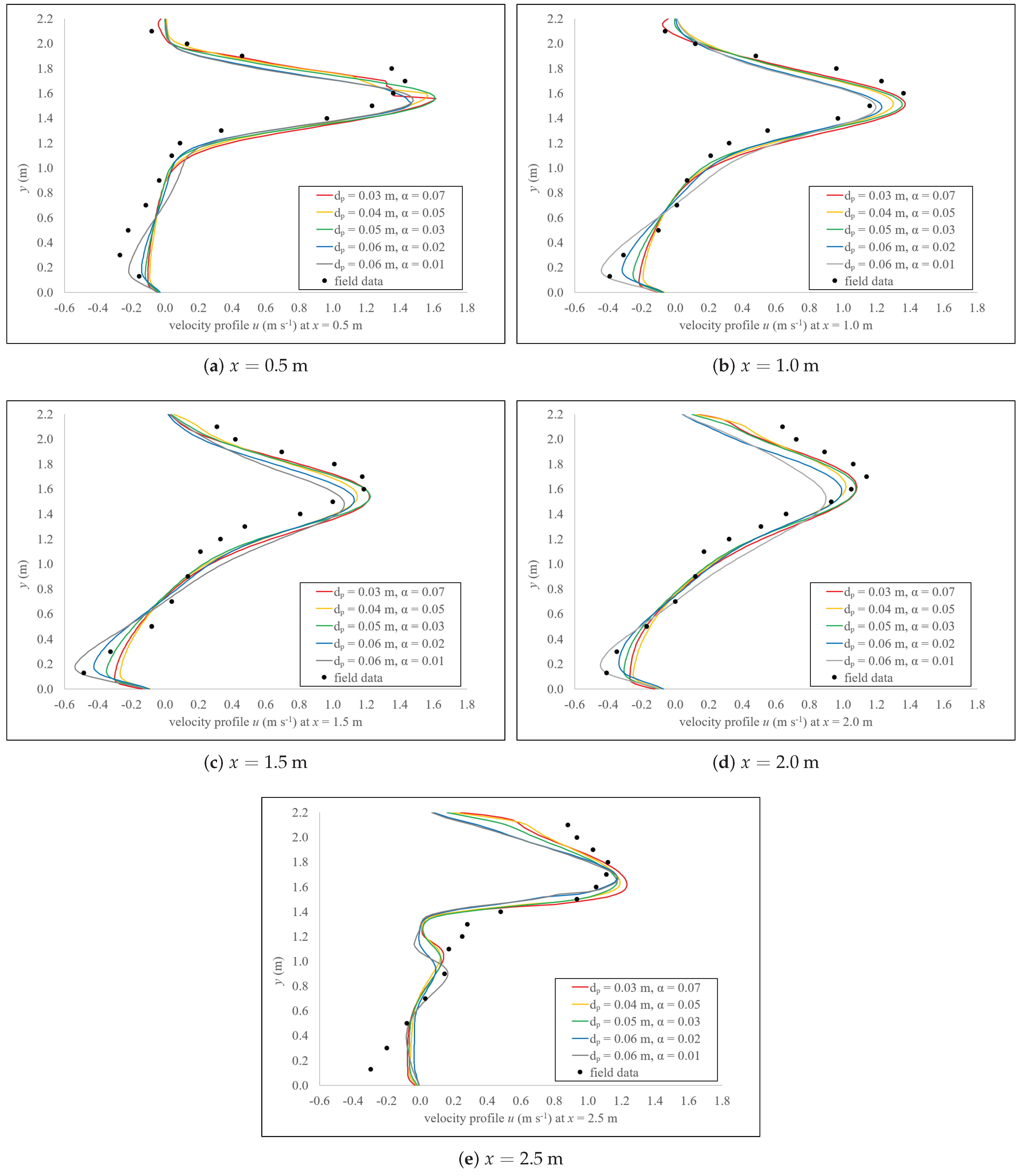
5.4. Effect of Particle Spacing and Artificial Viscosity Coefficient
Monaghan and Kajtar (2009) [61] and Crespo et al., (2011) [34] noticed a relation between artificial viscosity parameter and the Reynolds number of the flow. The results obtained in the present study confirm that in DualSPHysics the selection of (i.e., particle spacing) has to be accompanied by selection of an adequate value of (i.e., artificial viscosity coefficient) for a proper simulation outcome.
For smaller values of the initial particle spacing, resulting in an increased number of particles generated during the pre-processing, an adequately higher value of is required to generate consistent velocity profiles. This effect can be seen in Figure 11a–e, where plots of velocity profiles at different locations are superimposed for several values of the viscosity coefficient, varied according to the varying particle spacing. Velocity profiles are very similar for the following combinations of and : 1) m, , 2) m, , and 3) m, . Increasing even further to values of 0.06 m and beyond, and correspondingly decreasing to values 0.01 or less, generally gives much worse agreement in terms of velocity profiles, as can be seen from Table 3. These velocity profiles indicate that higher resolutions indeed lead to better results when coupled with an appropriately selected value , as also confirmed in Domínguez et al., (2019) [62].
5.5. Use of the Laminar Viscosity and SPS Turbulence Model
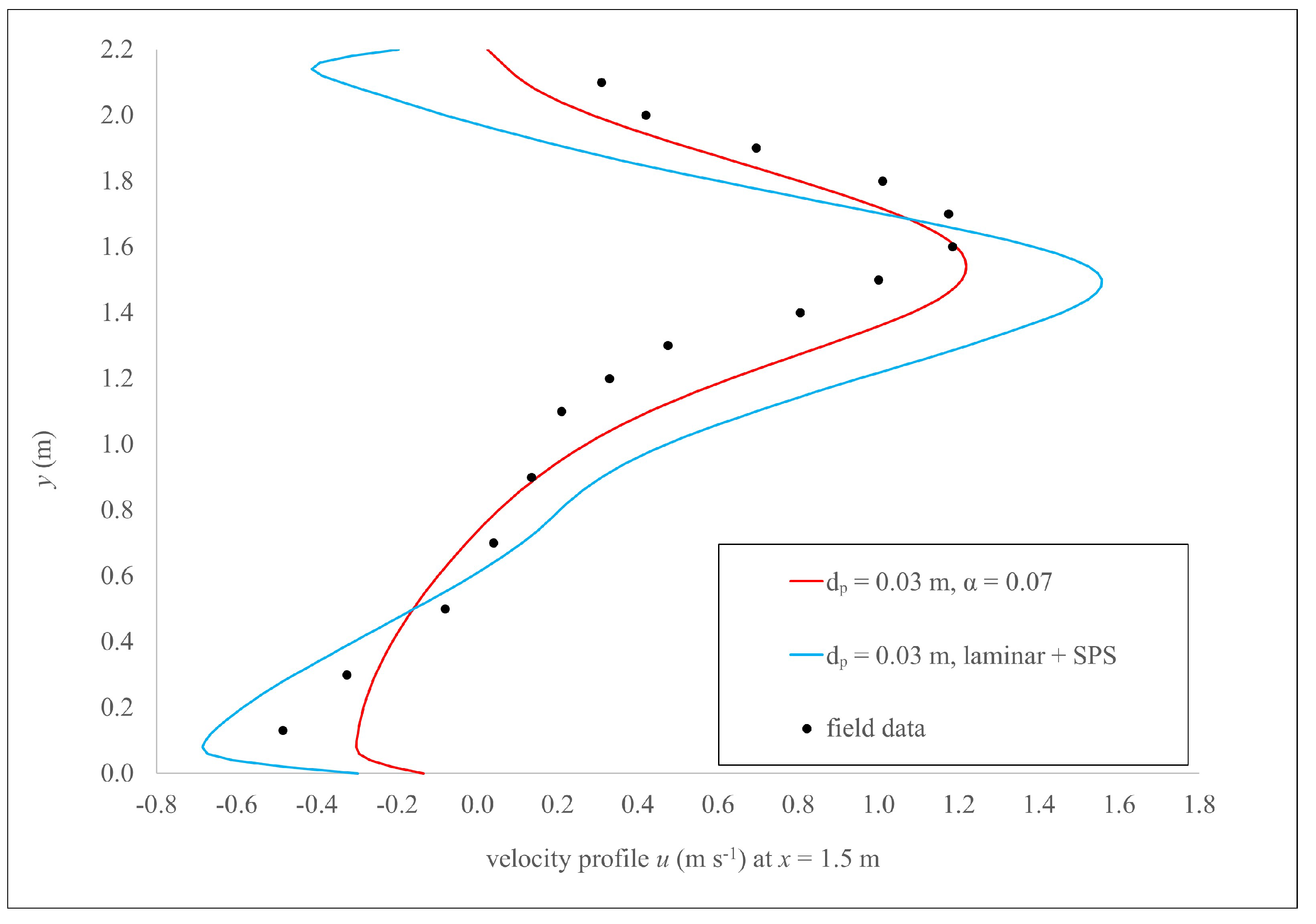
The laminar + SPS treatment of viscosity has been investigated with ranging from 0.03 m to 0.06 m. For these cases, the kinematic viscosity of water has been set to m/s. Results using the m with laminar + SPS option are presented in Figure 12. The plot shows that the results obtained using the artificial viscosity agree better with measurements than the results obtained with the laminar + SPS approach.
5.6. Relation between Particle Spacing and Artificial Viscosity Coefficient
As seen previously, various combinations of particle spacing and viscosity coefficient give similar velocity profiles. These combinations are arranged in a cohesive manner in Table 4. Based on this data, a relation between the number of fluid particles and the value which is required to reproduce the suitable velocity profiles can be obtained with a simple logarithmic fit of the form:
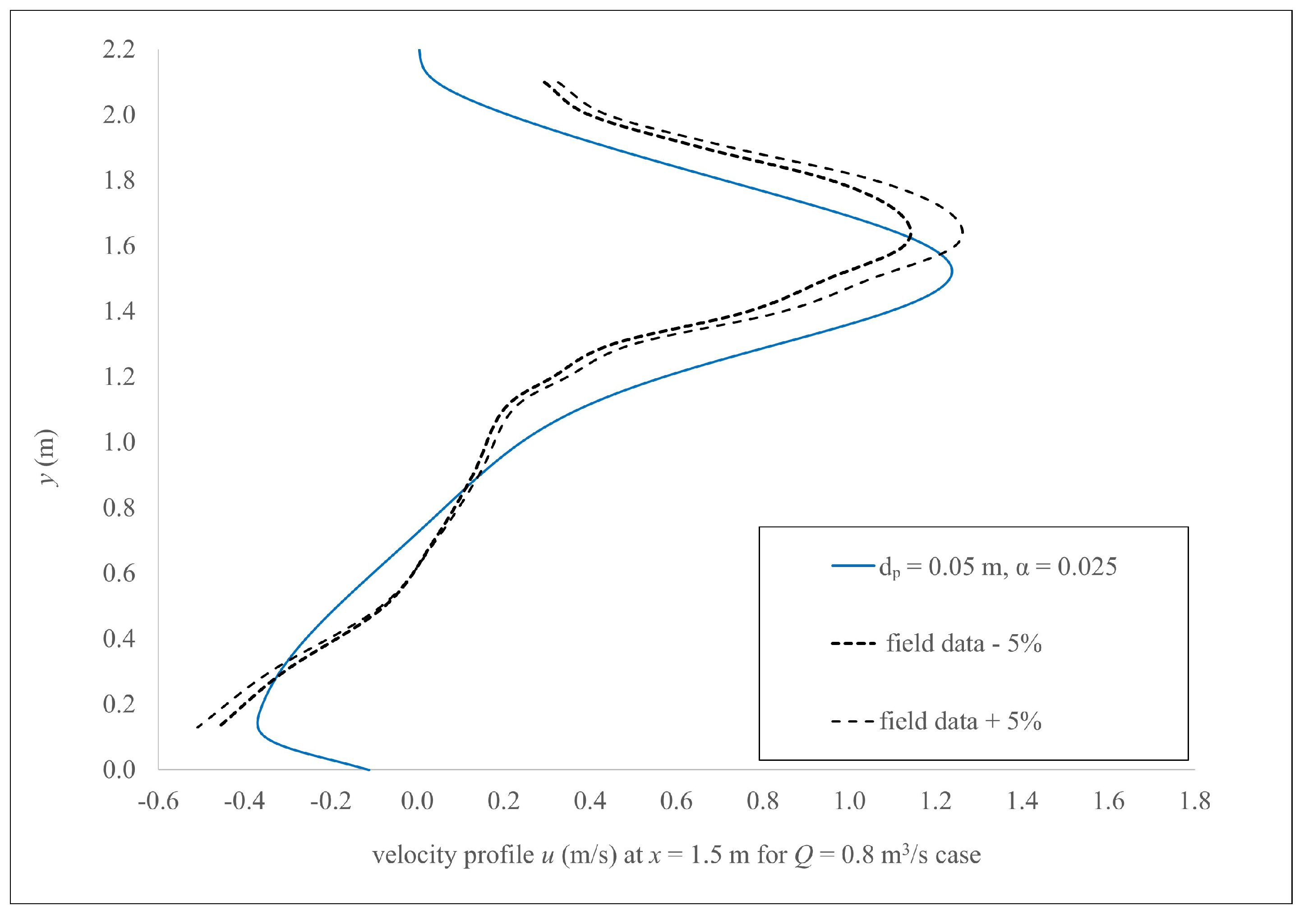
with a value of the R-square coefficient of approximately 0.991. To test the validity of Equation (12), an additional VSF case of m/s, m has been simulated, and compared against data by Bombač et al., (2015) [12]. Therein, a 2-D depth-averaged model was applied to confirm that velocity profiles in the observed VSF were very similar for various discharges ranging from 0.4 m/s to 2.0 m/s (difference between maximal values of u for these discharges was only 12 %), and that change of Q resulted only in a change of H, while velocities remained practically the same [18]. This translates into the possibility of using measured velocities from the m/s, m case (i.e., ADV points by Bombač et al., 2015 [12]) as an approximate reference frame against which the results from DualSPHysics model can be compared for the m/s, H = 1.06 m case. To achieve this, we decrease the values of imposed velocities and water elevations at inlet and outlet, since lower depth results in a smaller number of fluid particles. We then apply values of calculated from Equation (12). The total number of fluid particles is 133,628 and from Equation (12) a value of = 0.025 is obtained. The calculated discharge in the slot is equal to 0.74 m/s, and the velocity profile at m seen in Figure 13 is satisfactory as well. As mentioned above, results from depth-averaged model by Bombač et al., (2017) [18], here increased and decreased by 5 %, respectively (two dashed lines in Figure 13), act as an approximate reference frame. The authors would like to remark that no detailed sensitivity analysis was performed. Additional research is needed to widen the applicability of Equation (12). Nevertheless, the current research indicates that there is a relation between the particle spacing and the value of the artificial viscosity coefficient.
6. Conclusions
Fishways have a great ecological importance and have thus been the subject of many studies. However, many fishways are still not functioning properly, thus this research field remains relevant. In the present work, SPH-based 3-D solver DualSPHysics has been applied to numerically simulate flow in a vertical slot fishway (VSF). A versatile algorithm for the treatment of open boundary conditions using buffer layers has been applied to a case of free surface turbulent subcritical flow in a VSF to accurately reproduce discharges, water elevations and various velocity profiles (longitudinal and transverse velocities) within the observed pool of the VSF. This indicates DualSPHysics can be an accurate tool for modeling flows similar to those in VSF. Model has been successfully calibrated against the published field data of flow velocities that were measured with acoustic Doppler velocity probe. The effects of the main execution parameters, i.e., particle spacing and viscosity, have been investigated. Study shows that increasing the resolution of a model by decreasing the initial interparticle distance (and consequently increasing the number of fluid particles), should be coupled with an appropriately selected value of artificial viscosity coefficient to obtain the best results. An approach with laminar viscosity and SPS turbulence model has been examined as well, but this viscosity treatment has given velocity profiles that are not as accurate as in simulations using artificial viscosity. Based on the present study, a novel relation between the number of fluid particles and artificial viscosity coefficient has been formulated with a simple logarithmic fit. Currently, this relation indicates a trend that presents a useful guideline, but further studies including various geometries and types of flow should be performed to test its validity and to widen its applicability to a wider range of hydrodynamic problems.
Author Contributions
All authors listed have contributed substantially to the work reported. Conceptualization: G.N., A.T., D.Ž., M.Č.; methodology: A.T., J.M.D.; software: J.M.D., A.T.; results analysis: G.N., A.T.; visualization: A.T., G.N., J.M.D.; writing: G.N., A.T.; supervision: M.Č., D.Ž.; funding: D.Ž., M.Č.
Funding
This research was funded by the Slovenian Ministry of Education, Science and Sport and the Slovenian Research Agency as part of the research programme “Water Science and Technology, and Geotechnical Engineering: Tools and Methods for Process Analyses and Simulations, and Development of Technologies” (P2-0180).
Conflicts of Interest
The authors declare no conflict of interest.
Nomenclature
The following main nomenclature is used in this manuscript:
| coefficient of artificial viscosity (-) | |
| average numerical speed of sound (m s) | |
| initial interparticle distance (m) | |
| Wilcoxon test constant (-) | |
| g | acceleration of gravity (m s) |
| H | water elevation, depth (m) |
| Q | discharge (m s) |
| t | time (s) |
| u | longitudinal velocity (m s) |
| v | transverse velocity (m s) |
| w | vertical velocity (m s) |
| x | distance in longitudinal direction (m) |
| y | distance in transverse direction (m) |
| z | distance in vertical direction (m) |
Abbreviations
The following abbreviations are used in this manuscript:
| 2-D | Two-dimensional |
| 3-D | Three-dimensional |
| ADV | Acoustic Doppler velocimeter |
| CFD | Computational Fluid Dynamics |
| CPU | Central processing unit |
| CUDA | Compute unified device architecture |
| DBC | Dynamic boundary conditions |
| GPU | Graphics processing unit |
| GPGPU | General-purpose graphics processing unit |
| HPP | Hydropower plants |
| LES | Large eddy simulation |
| SPH | Smoothed particle hydrodynamics |
| SPS | Sub-particle scales |
| VSF | Vertical slot fishway |
| WCSPH | Weakly compressible SPH |
References
- D’Enno, D.; Marmulla, G.; Food and Agriculture Organization; Welcomme, R.; Food and Agriculture Organization of the United Nations; Deutscher Verband für Wasserwirtschaft und Kulturbau. Fish Passes: Design, Dimensions and Monitoring; Food and Agriculture Organization of the United Nations: Rome, Italy, 2002. [Google Scholar]
- Tan, J.; Tao, L.; Gao, Z.; Dai, H.; Shi, X. Modeling Fish Movement Trajectories in Relation to Hydraulic Response Relationships in an Experimental Fishway. Water 2018, 10, 1511. [Google Scholar] [CrossRef]
- Crowder, D.W.; Diplas, P. Applying spatial hydraulic principles to quantify stream habitat. River Res. Appl. 2006, 22, 79–89. [Google Scholar] [CrossRef]
- Shen, Y.; Diplas, P. Application of two- and three-dimensional computational fluid dynamics models to complex ecological stream flows. J. Hydrol. 2008, 348, 195–214. [Google Scholar] [CrossRef]
- Mao, X. Review of fishway research in China. Ecol. Eng. 2018, 115, 91–95. [Google Scholar] [CrossRef]
- Stamou, A.I.; Mitsopoulos, G.; Rutschmann, P.; Bui, M.D. Verification of a 3D CFD model for vertical slot fish-passes. Environ. Fluid Mech. 2018, 18, 1435–1461. [Google Scholar] [CrossRef]
- Sanagiotto, D.G.; Rossi, J.B.; Bravo, J.M. Applications of Computational Fluid Dynamics in The Design and Rehabilitation of Nonstandard Vertical Slot Fishways. Water 2019, 11, 199. [Google Scholar] [CrossRef]
- Odeh, M.; Noreika, J.; Haro, A.; Maynard, A.; Castro-Santos, T.; Cada, G. Evaluation of the Effects of Turbulence on the Behaviour of Migratory Fish; Technical Report DOE/BP-00000022-1; Bonneville Power Administration (BPA): Portland, OR, USA, 2002.
- Puertas, J.; Pena, L.; Teijeiro, T. Experimental Approach to the Hydraulics of Vertical Slot Fishways. J. Hydraul. Eng. 2004, 130, 10–23. [Google Scholar] [CrossRef]
- Tarrade, L.; Texier, A.; David, L.; Larinier, M. Topologies and measurements of turbulent flow in vertical slot fishways. Hydrobiologia 2008, 609, 177. [Google Scholar] [CrossRef]
- Chorda, J.; Maubourguet, M.M.; Roux, H.; Larinier, M.; Tarrade, L.; David, L. Two-dimensional free surface flow numerical model for vertical slot fishways. J. Hydraul. Res. 2010, 48, 141–151. [Google Scholar] [CrossRef] [Green Version]
- Bombač, M.; Novak, G.; Mlačnik, J.; Četina, M. Extensive field measurements of flow in vertical slot fishway as data for validation of numerical simulations. Ecol. Eng. 2015, 84, 476–484. [Google Scholar] [CrossRef]
- Marriner, B.A.; Baki, A.B.; Zhu, D.Z.; Cooke, S.J.; Katopodis, C. The hydraulics of a vertical slot fishway: A case study on the multi-species Vianney-Legendre fishway in Quebec, Canada. Ecol. Eng. 2016, 90, 190–202. [Google Scholar] [CrossRef]
- Wu, S.; Rajaratnam, N.; Katopodis, C. Structure of Flow in Vertical Slot Fishway. J. Hydraul. Eng. 1999, 125, 351–360. [Google Scholar] [CrossRef]
- Liu, M.; Rajaratnam, N.; Zhu, D.Z. Mean Flow and Turbulence Structure in Vertical Slot Fishways. J. Hydraul. Eng. 2006, 132, 765–777. [Google Scholar] [CrossRef]
- Cea, L.; Pena, L.; Puertas, J.; Vázquez-Cendón, M.E.; Peña, E. Application of Several Depth-Averaged Turbulence Models to Simulate Flow in Vertical Slot Fishways. J. Hydraul. Eng. 2007, 133, 160–172. [Google Scholar] [CrossRef]
- Bermúdez, M.; Puertas, J.; Cea, L.; Pena, L.; Balairón, L. Influence of pool geometry on the biological efficiency of vertical slot fishways. Ecol. Eng. 2010, 36, 1355–1364. [Google Scholar] [CrossRef]
- Bombač, M.; Četina, M.; Novak, G. Study on flow characteristics in vertical slot fishways regarding slot layout optimization. Ecol. Eng. 2017, 107, 126–136. [Google Scholar] [CrossRef]
- Masayuki, F.; Mai, A.; Mattashi, I. Chapter 3-D Flow Simulation of an Ice-Harbor Fishway. In Advances in Water Resources and Hydraulic Engineering; Springer: Berlin, Germany, 2009; pp. 2241–2246. [Google Scholar]
- Ferrand, M.; Laurence, D.R.; Rogers, B.D.; Violeau, D.; Kassiotis, C. Unified semi-analytical wall boundary conditions for inviscid, laminar or turbulent flows in the meshless SPH method. Int. J. Numer. Methods Fluids 2013, 71, 446–472. [Google Scholar] [CrossRef]
- Duguay, J.; Lacey, R.; Gaucher, J. A case study of a pool and weir fishway modeled with OpenFOAM and FLOW-3D. Ecol. Eng. 2017, 103, 31–42. [Google Scholar] [CrossRef]
- Gisen, D.C.; Weichert, R.B.; Nestler, J.M. Optimizing attraction flow for upstream fish passage at a hydropower dam employing 3D Detached-Eddy Simulation. Ecol. Eng. 2017, 100, 344–353. [Google Scholar] [CrossRef] [Green Version]
- Umeda, Y.C.L.; de Lima, G.; Janzen, J.G.; Salla, M.R. One- and three-dimensional modelling of a vertical-slot fishway. J. Urban Environ. Eng. 2017, 11, 99–107. [Google Scholar] [CrossRef]
- Li, Y.; Wang, X.; Xuan, G.; Liang, D. Effect of parameters of pool geometry on flow characteristics in low slope vertical slot fishways. J. Hydraul. Res. 2019, 1–13. [Google Scholar] [CrossRef]
- Romão, F.; Santos, J.M.; Katopodis, C.; Pinheiro, A.N.; Branco, P. How Does Season Affect Passage Performance and Fatigue of Potamodromous Cyprinids? An Experimental Approach in a Vertical Slot Fishway. Water 2018, 10, 395. [Google Scholar] [CrossRef]
- Ceola, S.; Pugliese, A.; Ventura, M.; Galeati, G.; Montanari, A.; Castellarin, A. Hydro-power production and fish habitat suitability: Assessing impact and effectiveness of ecological flows at regional scale. Adv. Water Resour. 2018, 116, 29–39. [Google Scholar] [CrossRef]
- Scholten, M.; Schütz, C.; Wassermann, S.; Weichert, R. Improving ecological continuity in German waterways: Research challenges of upstream migration and fishway. In Proceedings of the 10th International Symposium on Ecohydraulics, Norway, Trondheim, 23–27 November 2014. [Google Scholar]
- Kolman, G.; Mikoš, M.; Povž, M. Fish passages on hydroelectric power dams in Slovenia. Nat. Conserv. 2010, 24, 85–96. [Google Scholar]
- Ciuha, D.; Povž, M.; Kvaternik, K.; Brenčič, M.; Muck, P. The design and technical solutions of passages for aquatic organisms at the HPP on the lower Sava River reach, with an emphasis on the passage at HPP Arto—Blanca. In Proceedings of the Mišičev Vodarski Dan (in Slovenian), Maribor, Slovenia, 4 December 2014; pp. 228–236. [Google Scholar]
- Tafuni, A.; Sahin, I. Non-linear hydrodynamics of thin laminae undergoing large harmonic oscillations in a viscous fluid. J. Fluids Struct. 2015, 52, 101–117. [Google Scholar] [CrossRef]
- Canelas, R.B.; Domínguez, J.M.; Crespo, A.J.C.; Gómez-Gesteira, M.; Ferreira, R.M.L. Resolved Simulation of a Granular-Fluid Flow with a Coupled SPH-DCDEM Model. J. Hydraul. Eng. 2017, 143, 06017012. [Google Scholar] [CrossRef]
- Sun, P.; Zhang, A.M.; Marrone, S.; Ming, F. An accurate and efficient SPH modeling of the water entry of circular cylinders. Appl. Ocean Res. 2018, 72, 60–75. [Google Scholar] [CrossRef]
- González-Cao, J.; Altomare, C.; Crespo, A.; Domínguez, J.; Gómez-Gesteira, M.; Kisacik, D. On the accuracy of DualSPHysics to assess violent collisions with coastal structures. Comput. Fluids 2019, 179, 604–612. [Google Scholar] [CrossRef]
- Crespo, A.J.C.; Dominguez, J.M.; Barreiro, A.; Gómez-Gesteira, M.; Rogers, B.D. GPUs, a New Tool of Acceleration in CFD: Efficiency and Reliability on Smoothed Particle Hydrodynamics Methods. PLoS ONE 2011, 6, e20685. [Google Scholar] [CrossRef]
- Domínguez, J.M.; Crespo, A.J.C.; Gómez-Gesteira, M. Optimization strategies for CPU and GPU implementations of a smoothed particle hydrodynamics method. Comput. Phys. Commun. 2013, 184, 617–627. [Google Scholar] [CrossRef]
- Domínguez, J.M.; Crespo, A.J.C.; Valdez-Balderas, D.; Rogers, B.D.; Gómez-Gesteira, M. New multi-GPU implementation for smoothed particle hydrodynamics on heterogeneous clusters. Comput. Phys. Commun. 2013, 184, 1848–1860. [Google Scholar] [CrossRef]
- Marivela, R.; López, D. Applications of the SPH model to fishways design. In Proceedings of the XIII World Forestry Congress, Buenos Aires, Argentina, 18–25 October 2009. [Google Scholar]
- Violeau, D.; Issa, R.; Benhamadouche, S.; Saleh, K.; Chorda, J.; Maubourguet, M.M. Modelling a fish passage with SPH and Eulerian codes: The influence of turbulent closure. In Proceedings of the 3rd SPHERIC International Workshop, Lausanne, Switzerland, 4–6 June 2008. [Google Scholar]
- Gomes, D.; Nascimento, G. Application of a Meshless CFD Method for a Vertical Slot Fish Pass via 3D Simulation. Int. J. Sci. Eng. Investig. 2018, 7, 147–151. [Google Scholar]
- Crespo, A.J.C.; Domínguez, J.M.; Rogers, B.D.; Gómez-Gesteira, M.; Longshaw, S.; Canelas, R.; Vacondio, R.; Barreiro, A.; García-Feal, O. DualSPHysics: Open-source parallel CFD solver based on Smoothed Particle Hydrodynamics SPH. Comput. Phys. Commun. 2015, 187, 204–216. [Google Scholar] [CrossRef]
- Monaghan, J.; Lattanzio, J. A Refined Particle Method for Astrophysical Problems. Astron. Astrophys. 1985, 149, 135–143. [Google Scholar]
- Wendland, H. Piecewise polynomial, positive definite and compactly supported radial functions of minimal degree. Adv. Comput. Math. 1995, 4, 389–396. [Google Scholar] [CrossRef]
- Monaghan, J.J. Smoothed Particle Hydrodynamics. Annu. Rev. Astron. Astrophys. 1992, 30, 543–574. [Google Scholar] [CrossRef]
- Altomare, C.; Crespo, A.J.C.; Domínguez, J.M.; Gómez-Gesteira, M.; Suzuki, T.; Verwaest, T. Applicability of smoothed particle hydrodynamics for estimation of sea wave impact on coastal structures. Coast. Eng. 2015, 96, 1–12. [Google Scholar] [CrossRef]
- Monaghan, J.J. Simulating free surface flows with SPH. J. Comput. Phys. 1994, 110, 399–406. [Google Scholar] [CrossRef]
- Gotoh, H.; Shao, S.; Memita, T. SPH-LES Model for Numerical Investigation of Wave Interaction with Partially Immersed Breakwater. Coast. Eng. J. 2004, 46, 39–63. [Google Scholar] [CrossRef]
- Dalrymple, R.A.; Rogers, B.D. Numerical modeling of water waves with the SPH method. Coast. Eng. 2006, 53, 141–147. [Google Scholar] [CrossRef]
- Molteni, D.; Colagrossi, A. A simple procedure to improve the pressure evaluation in hydrodynamic context using the SPH. Comput. Phys. Commun. 2009, 180, 861–872. [Google Scholar] [CrossRef]
- Marrone, S.; Antuono, M.; Colagrossi, A.; Colicchio, G.; Touzé, D.L.; Graziani, G. δ-SPH model for simulating violent impact flows. Comput. Methods Appl. Mech. Eng. 2011, 200, 1526–1542. [Google Scholar] [CrossRef]
- Fourtakas, G.; Rogers, B. Modelling multi-phase liquid-sediment scour and resuspension induced by rapid flows using Smoothed Particle Hydrodynamics (SPH) accelerated with a Graphics Processing Unit (GPU). Adv. Water Resour. 2016, 92, 186–199. [Google Scholar] [CrossRef]
- Mokos, A.; Rogers, B.D.; Stansby, P.K. A multi-phase particle shifting algorithm for SPH simulations of violent hydrodynamics with a large number of particles. J. Hydraul. Res. 2017, 55, 143–162. [Google Scholar] [CrossRef]
- Buruchenko, S.K.; Crespo, A.J.C. Validation DualSPHysics code for liquid sloshing phenomena. In Proceedings of the ICCM2014, Cambridge, UK, 28–30 July 2014. [Google Scholar]
- Mogan, S.C.; Chen, D.; Hartwig, J.; Sahin, I.; Tafuni, A. Hydrodynamic analysis and optimization of the Titan submarine via the SPH and Finite–Volume methods. Comput. Fluids 2018, 174, 271–282. [Google Scholar] [CrossRef]
- Tafuni, A.; Sahin, I.; Hyman, M. Numerical investigation of wave elevation and bottom pressure generated by a planing hull in finite-depth water. Appl. Ocean Res. 2016, 58, 281–291. [Google Scholar] [CrossRef]
- Verbrugghe, T.; Domínguez, J.M.; Crespo, A.J.; Altomare, C.; Stratigaki, V.; Troch, P.; Kortenhaus, A. Coupling methodology for smoothed particle hydrodynamics modelling of non-linear wave-structure interactions. Coast. Eng. 2018, 138, 184–198. [Google Scholar] [CrossRef]
- Verbrugghe, T.; Domínguez, J.; Altomare, C.; Tafuni, A.; Vacondio, R.; Troch, P.; Kortenhaus, A. Non-linear wave generation and absorption using open boundaries within DualSPHysics. Comput. Phys. Commun. 2019, 240, 46–59. [Google Scholar] [CrossRef]
- Novak, G.; Žagar, D.; Četina, M.; Bombač, M. Vertical slot fishway simulated with PCFLOW2D and DualSPHysics v4.2 models. In Proceedings of the Panama 2019 IAHR World Congress, Urb. Marbella, Panamá, 1–6 September 2019. [Google Scholar]
- Tafuni, A.; Domínguez, J.M.; Vacondio, R.; Crespo, A.J.C. A versatile algorithm for the treatment of open boundary conditions in Smoothed particle hydrodynamics GPU models. Comput. Methods Appl. Mech. Eng. 2018, 342, 604–624. [Google Scholar] [CrossRef]
- Crespo, A.J.C.; Gómez-Gesteira, M.; Dalrymple, R.A. Boundary conditions generated by dynamic particles in SPH methods. Comput. Mater. Contin. 2007, 5, 173–184. [Google Scholar] [CrossRef]
- Altomare, C.; Crespo, A.J.C.; Rogers, B.D.; Domínguez, J.M.; Gironella, X.; Gómez-Gesteira, M. Numerical modelling of armour block sea breakwater with smoothed particle hydrodynamics. Comput. Struct. 2014, 130, 34–45. [Google Scholar] [CrossRef]
- Monaghan, J.; Kajtar, J. SPH particle boundary forces for arbitrary boundaries. Comput. Phys. Commun. 2009, 180, 1811–1820. [Google Scholar] [CrossRef]
- Domínguez, J.M.; Altomare, C.; Gonzalez-Cao, J.; Lomonaco, P. Towards a more complete tool for coastal engineering: Solitary wave generation, propagation and breaking in an SPH-based model. Coast. Eng. J. 2019, 61, 15–40. [Google Scholar] [CrossRef]
Figure 1.
Locations of flow velocity measurements by Bombač et al., (2015) [12].
Figure 1.
Locations of flow velocity measurements by Bombač et al., (2015) [12].

Figure 2.
Plan view of the VSF, showing the coordinate system with a base at the corner of the pool, locations of observed cross sections m, 1.0 m, 1.5 m, 2.0 m and 2.5 m, and profiles m, 1.10 m, 1.65 m. Dimensions are in meters.
Figure 2.
Plan view of the VSF, showing the coordinate system with a base at the corner of the pool, locations of observed cross sections m, 1.0 m, 1.5 m, 2.0 m and 2.5 m, and profiles m, 1.10 m, 1.65 m. Dimensions are in meters.

Figure 3.
Contour maps of flow variables at the free surface (top view). Left panels represent velocity magnitude, colored from 0 m/s (blue) to 1.5 m/s (red). Right panels show contours of vorticity in z, from −3 rad/s (blue) to 3 rad/s (red).
Figure 3.
Contour maps of flow variables at the free surface (top view). Left panels represent velocity magnitude, colored from 0 m/s (blue) to 1.5 m/s (red). Right panels show contours of vorticity in z, from −3 rad/s (blue) to 3 rad/s (red).

Figure 4.
Contour maps of flow variables at m from the free surface (top view). Left panels represent velocity magnitude, colored from 0 m/s (blue) to 1.5 m/s (red). Right panels show contours of vorticity in z, from −3 rad/s (blue) to 3 rad/s (red).
Figure 4.
Contour maps of flow variables at m from the free surface (top view). Left panels represent velocity magnitude, colored from 0 m/s (blue) to 1.5 m/s (red). Right panels show contours of vorticity in z, from −3 rad/s (blue) to 3 rad/s (red).

Figure 5.
Discharge in the numerical pool as observed from the calibrated model.

Figure 6.
Water depth profiles along m, m, and m.

Figure 7.
Prototype VSF at Arto–Blanca HPP during field measurements.

Figure 8.
Measured (Bombač et al., 2015) and calculated u and v velocity profiles.

Figure 9.
Velocity magnitude against vertical distance at different x locations. Red curves with circles are SPH velocities, blue curves with squares are experimental velocities.
Figure 9.
Velocity magnitude against vertical distance at different x locations. Red curves with circles are SPH velocities, blue curves with squares are experimental velocities.

Figure 10.
Calculated profiles of u at various depths z near the slot region.

Figure 11.
Average velocity profile of u at different x positions and for several different values of and compared against field data.
Figure 11.
Average velocity profile of u at different x positions and for several different values of and compared against field data.

Figure 12.
Average velocity profiles with artificial and laminar + SPS treatment of viscosity, both compared against field data.
Figure 12.
Average velocity profiles with artificial and laminar + SPS treatment of viscosity, both compared against field data.

Figure 13.
Average velocity profile for the m/s, m case.


Table 1.
Measured (ADV) and calculated (SPH) average values of u in m/s for the calibrated model.
| Location | m | m | m | m | m | |||||
|---|---|---|---|---|---|---|---|---|---|---|
| ADV | SPH | ADV | SPH | ADV | SPH | ADV | SPH | ADV | SPH | |
| m | 1.43 | 1.23 | 1.23 | 0.99 | 1.18 | 1.02 | 1.14 | 1.03 | 1.11 | 1.15 |
| m | 1.36 | 1.58 | 1.36 | 1.26 | 1.19 | 1.19 | 1.05 | 1.08 | 1.05 | 1.15 |
| m | −0.08 | 0.00 | −0.06 | 0.02 | 0.31 | 0.15 | 0.64 | 0.34 | 0.88 | 0.51 |
| m | −0.16 | −0.12 | −0.39 | −0.25 | −0.49 | −0.35 | −0.41 | −0.30 | −0.30 | −0.06 |
Table 2.
Two-tailed Wilcoxon signed-ranks test for paired samples with . Values in cells represent the test statistic, critical statistic (in brackets), and whether there is a significant difference, i.e., yes/no.
Table 2.
Two-tailed Wilcoxon signed-ranks test for paired samples with . Values in cells represent the test statistic, critical statistic (in brackets), and whether there is a significant difference, i.e., yes/no.
| m | m | m | m | m | |
|---|---|---|---|---|---|
| u | 40 (29); no | 52 (29); no | 52 (25); no | 66 (29); no | 31 (29); no |
| v | 31 (25); no | 13 (25); yes | 14 (25); yes | 12 (29); yes | 46 (29); no |
Table 3.
L-norm for the average profile of u for various combinations of and .
| [m] () | 0.03 (0.07) | 0.04 (0.05) | 0.05 (0.03) | 0.06 (0.02) | 0.06 (0.01) |
|---|---|---|---|---|---|
| L-norm | 12.1 | 11.7 | 11.9 | 14.1 | 15.6 |
Table 4.
Relation between particle spacing, , number of fluid particles, and viscosity coefficient, .
Table 4.
Relation between particle spacing, , number of fluid particles, and viscosity coefficient, .
| [m] | # of Fluid Particles | |
|---|---|---|
| 0.06 | 86,482 | 0.01 |
| 0.05 | 158,188 | 0.03 |
| 0.04 | 306,128 | 0.05 |
| 0.03 | 761,824 | 0.07 |
© 2019 by the authors. Licensee MDPI, Basel, Switzerland. This article is an open access article distributed under the terms and conditions of the Creative Commons Attribution (CC BY) license (http://creativecommons.org/licenses/by/4.0/).
Share and Cite
MDPI and ACS Style
Novak, G.; Tafuni, A.; Domínguez, J.M.; Četina, M.; Žagar, D. A Numerical Study of Fluid Flow in a Vertical Slot Fishway with the Smoothed Particle Hydrodynamics Method. Water 2019, 11, 1928. https://doi.org/10.3390/w11091928
AMA Style
Novak G, Tafuni A, Domínguez JM, Četina M, Žagar D. A Numerical Study of Fluid Flow in a Vertical Slot Fishway with the Smoothed Particle Hydrodynamics Method. Water. 2019; 11(9):1928. https://doi.org/10.3390/w11091928
Chicago/Turabian StyleNovak, Gorazd, Angelantonio Tafuni, José M. Domínguez, Matjaž Četina, and Dušan Žagar. 2019. "A Numerical Study of Fluid Flow in a Vertical Slot Fishway with the Smoothed Particle Hydrodynamics Method" Water 11, no. 9: 1928. https://doi.org/10.3390/w11091928
Note that from the first issue of 2016, this journal uses article numbers instead of page numbers. See further details here.