Analysis of the Effects of High Precipitation in Texas on Rainfed Sorghum Yields
by
 ,
,
Om Prakash Sharma
1, 
Narayanan Kannan
2,*,
Scott Cook
3,
Bijay Kumar Pokhrel
2 and
Cameron McKenzie
4 1
Department of Chemistry, Geosciences and Physics, Tarleton State University, Stephenville, TX 76402, USA
2
Texas Institute for Applied Environmental Research (TIAER), Tarleton State University, Stephenville, TX 76402, USA
3
Department of Mathematics, Tarleton State University, Stephenville, TX 76402, USA
4
Department of History, Sociology, Geography and GIS, Tarleton State University, Stephenville, TX 76402, USA
*
Author to whom correspondence should be addressed.
Water 2019, 11(9), 1920; https://doi.org/10.3390/w11091920
Submission received: 31 July 2019
/
Revised: 5 September 2019
/
Accepted: 10 September 2019
/
Published: 14 September 2019
(This article belongs to the Special Issue Water Management for Sustainable Food Production)
Abstract
:Most of the recent studies on the consequences of extreme weather events on crop yields are focused on droughts and warming climate. The knowledge of the consequences of excess precipitation on the crop yield is lacking. We attempted to fill this gap by estimating reductions in rainfed grain sorghum yields for excess precipitation. The historical grain sorghum yield and corresponding historical precipitation data are collected by county. These data are sorted based on length of the record and missing values and arranged for the period 1973–2003. Grain sorghum growing periods in the different parts of Texas is estimated based on the east-west precipitation gradient, north-south temperature gradient, and typical planting and harvesting dates in Texas. We estimated the growing season total precipitation and maximum 4-day total precipitation for each county growing rainfed grain sorghum. These two parameters were used as independent variables, and crop yields of sorghum was used as the dependent variable. We tried to find the relationships between excess precipitation and decreases in crop yields using both graphical and mathematical relationships. The result were analyzed in four different levels; 1. Storm by storm consequences on the crop yield; 2. Growing season total precipitation and crop yield; 3. Maximum 4-day precipitation and crop yield; and 4. Multiple linear regression of independent variables with and without a principal component analysis (to remove the correlations between independent variables) and the dependent variable. The graphical and mathematical results show decreases in rainfed sorghum yields in Texas for excess precipitation could be between 18% and 38%.
1. Introduction
Sorghum is a crop that can be grown as either a grain or cash crop. It is one of the top five cereal crops in the world. Sorghum is also required for the survival of humankind in different parts of the world, especially in Africa and Asia. The United States (US) is the largest producer of sorghum in the world [1]. In the US, sorghum usually grows throughout the sorghum belt from South Dakota to southern Texas [2]. The top five sorghum producing states are Kansas, Texas, Colorado, Oklahoma, and South Dakota. In the US, sorghum grain is primarily used for feeding of livestock and ethanol production, but it is becoming popular in the consumer food industry and other markets [3]. The livestock industry is one of the oldest standing marketplaces for sorghum grain in the US. Sorghum is utilized in feed rations for poultry, beef, dairy, and swine [3]. Also, a large portion of sorghum is used for biofuel production. It is also exported to the different parts of the world, including Mexico, China, and Japan.
Sorghum grain is highly resistant to drought and can withstand waterlogging better than any other cereal crop. Sorghum has a special fibrous root system, which can extend to a depth of 1.2 to 1.8 m (4 to 6 feet) deep in the soil. More than 75% of water and nutrients taken by root system are from the top 0.9 m (3 feet). Therefore, the deep extension of the root system helps sorghum withstand drought conditions better than any other cash crops [4]. Grain sorghum exhibits yield stability greater than maize. Drought resistance and heat tolerance make it a popular choice for marginal rainfall areas of semiarid zones of Africa where food shortages are common.
Total water use by a sorghum crop depends on the variety, maturation, planting date, and geographical and environmental conditions. It is estimated that the total use of 1750 mm/ha (28 inches of water/acre) water is needed for good sorghum yield of 783 kg/ha (700 lb/acre) [5]. The water use of sorghum depends on the growth stage of the sorghum plant (Table 1). During the early part of plant development, water use is relatively low but water stress during this time can affect plant growth and yield. Rainfall of 25 to 50 mm (1 to 2 inches) in the second week following sorghum pollination would result in the best yield if the period of pollination had adequate soil moisture [5,6]. The period from sorghum pollination to maturity is about 60 days. At the time of growth, a dry spell in the field from 14 to 60 days after pollination may have a small effect on the final harvesting yield of the sorghum crop. If no rain were to occur during the final period of 46 days, the yield of the sorghum crop would be greatly reduced [5,6]. Therefore, rainfall and its timing are important factors for the growth and yield of sorghum.
Although sorghum is tolerant of some waterlogging, it suffers damage under prolonged wetting of soil under very high rainfall [6]. Researchers from Australia, Germany, and the US have quantified the overall of extremes climate effects like drought, heat wave problems and precipitation on the crop yield variability of different staple crops around the world [7]. The year-to-year overall changes in the climatic factor in the growing season of maize, rice, sorghum, and wheat accounted the fluctuations of 20% to 49% of total yields [8]. Climatic extremes like hot and cold climates, drought, and heavy rainfall accounted for 18% to 43% of inter-annual variations in different crops yields [9]. Therefore, it is important to understand the consequences of climate extremes on crop yields to secure our food supply. A large body of literature already exists for drought. However, studies on the consequences of extremely high precipitation on crop yield are sparse, especially for grain sorghum. Therefore, an attempt is made in this study to analyze the consequences of high precipitation on rainfed grain sorghum yields.
Extreme precipitation events are producing more and more rain, and are now becoming one of the most common events since the beginning of the 1950s in many regions of the world, including the US. Scientists expect heavy rainfall as a consequence of a warming planet [10,11]. Warmer air mass can hold more water vapor content than cold air mass. For each degree of warming in the earth, the air mass capacity for holding water vapor goes up by about 7%. An atmosphere with more moist air can produce more heavy and continuous rainfall events, which is what has been observed all over the world since the 1950s [10,11].
An increase in continuous heavy rainfall events may not always show the increases in total rainfall over a season or year. Some studies show a small decrease in rainfall and show an increase of dry periods, which offsets rainfall increases falling during heavy events. The most immediate effect of heavy rainfall is the flooding. There are several recent examples of heavy rainfall events. In August 2017, Hurricane Harvey produced 1220 mm (48 inches) of heavy rainfall on Houston, Texas from a single event and was the biggest threat from tropical cyclones. In July 2016, more than 150 mm (6 inches) of heavy rainfall occurred in less than two hours in Ellicott City, Maryland, the estimated cost of the damage is more than $22 million dollars. In summary, we incur a huge economic loss because of heavy precipitation events, including some losses coming from a reduction in crop yields.
Precipitation is generally useful in recharging the soil profile, which is very important for crop growth. The precipitation efficiency in recharging the soil profile depends on intensity and rate at which precipitation occurs. Precipitation that falls on the soil at rates greater than 127 cm/h (0.5 inches an hour) are less efficient compared to lighter rain, because the water that runs off from the surface carries the fertile soil to the streams, lakes, and rivers which decreases future yields. The timing of rainfall while crops are growing is critical. During germination and stand establishment, either heavy rainfall or little rainfall can substantially affect the yield.
In general, the more precipitation during the crop growing season, the better the crop growth. However, too much precipitation will damage the crop by saturating the soil profile and removing air, which is also important for healthy plant growth. The majority of the previous studies relating extreme climate events and food production are focused on increasing temperatures and drought. The consequences of high precipitation on probable reduction in crop yields are often ignored. There is a big knowledge gap of understanding the consequences of extremely high precipitation on the yield of food crops and relating it to subsequent consequences in food production scenarios at different spatial scales. Addressing the knowledge gap and exploring the less-studied relationship between excess precipitation and rainfed food crop yields are the novelties of this study. Detailed analysis of the above-mentioned relationship using a combination of established mathematical principles and graphical tools are some of the unique aspects of this study. The results from our study and other similar studies have applications in crop insurance, parameterization of computer models (estimating crop yield reductions based on aeration stress), policy level decisions on rainfed crop selection, yield forecasting, estimating food production, and water footprint analysis.
The specific objectives of the study are to: (1) Identify historic extreme high precipitation events during the crop growth of rainfed sorghum in Texas, (2) Extract continuous serially complete crop yield information for rainfed sorghum by county, (3) Collect continuous records of daily average precipitation corresponding to the sorghum crop yield data, (4) Estimate the growing season total precipitation and 4-day maximum precipitation using the precipitation data, and (5) Relate items 3 and 4 above using visual patterns and statistical principles to quantify the consequences of high precipitation on crop yields.
2. Materials and Methods
2.1. Data Collection and Arrangement
2.1.1. GIS Data
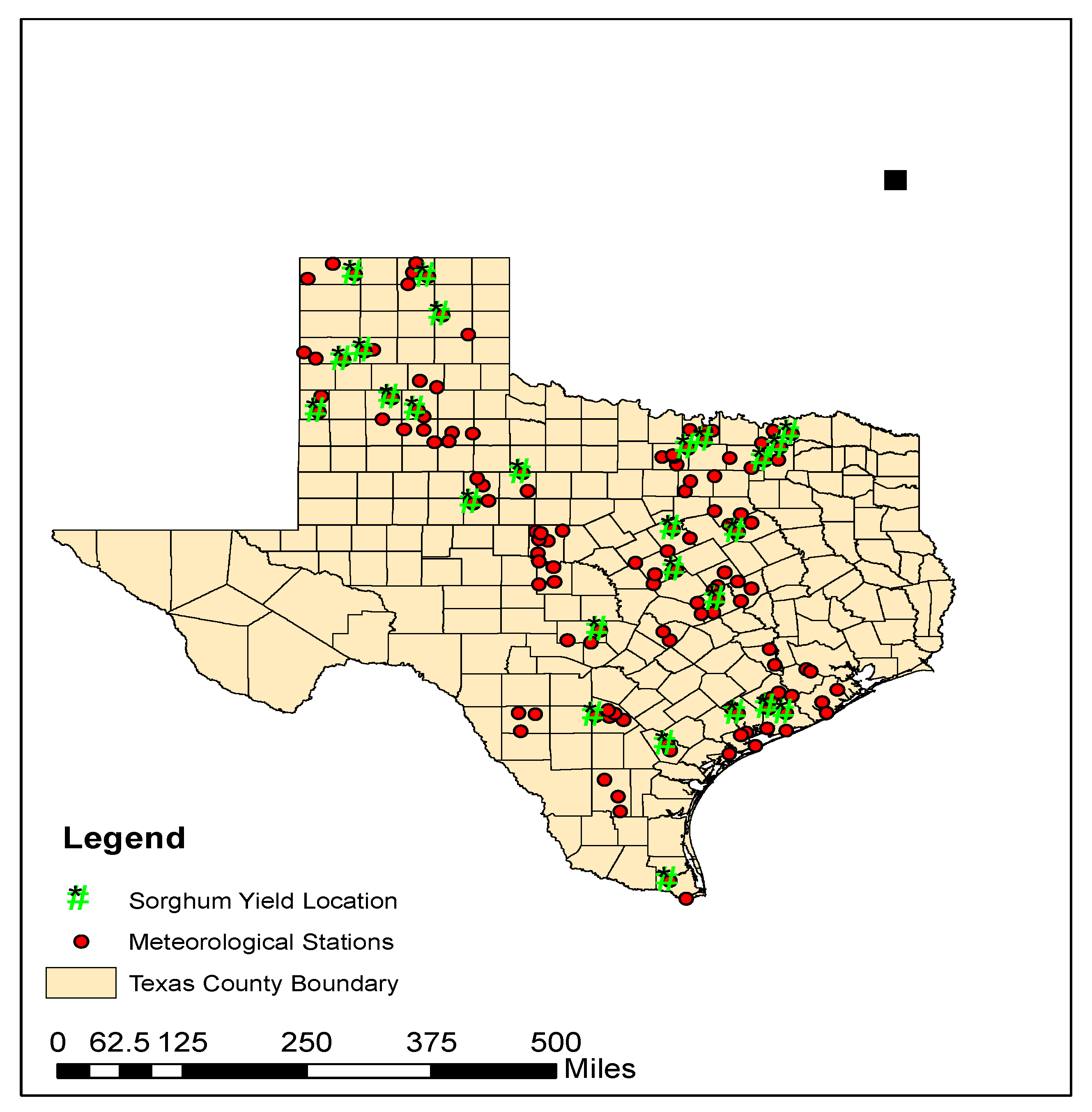
The map of county boundaries was downloaded from the Texas Natural Resources Information System (TNRIS) website [12]. The cultivated area map of Texas was downloaded from the National Land Cover Dataset (NLCD) [13] and overlaid with county boundaries. A map showing the location of meteorological stations in Texas was developed using the latitude and longitude information that came with the precipitation data. It was overlaid with county boundaries to identify the list of weather stations within each county. Continuous records of Sorghum yield data (without gaps) are required for the analysis. In addition, the data availability period had to be consistent for different counties in Texas. The period from 1973 to 2000 satisfied the criteria of no data gaps and consistent availability of data for many counties. Therefore, only those counties with rainfed sorghum yield data (Figure 1, Table A1 in Appendix A) for the period 1973–2000 are included in the analysis and 26 United State Geological Survey (USGS) precipitation gaging data satisfied these criteria are considered for further analysis. Twenty-six meteorological stations (precipitation data from USGS) correspond to the counties having rainfed sorghum yield.
2.1.2. Estimation of Sorghum Growing Season for Different Counties in Texas
Grain sorghum is a hot season crop grown in most arid plain states that do not have enough moisture to grow other crops. Sorghum is planted once the soil temperature is consistent at about 15.5 °C (60 °F). This sometimes depends on the local condition so it can occur as early as late February in warmer climates or May in colder climates. This crop has longer maturity stages than other corn and cereal crops.
The planting dates of sorghum were estimated from USDA-ARS [14], taking into consideration the north-south temperature gradient. The harvest dates were estimated based on the planting date and the crop duration of 120 days (assumption). The detail of dates of planting and harvesting estimated for different counties in Texas are shown below in Table 2.
There is a north-south temperature gradient in Texas. Therefore, planting starts from the south and moves toward the northern region of Texas. Sorghum is planted in the southern region of Texas first around the last week of March and then towards the south-central region followed by the far eastern and eastern regions and finally ends toward the north in the last week of May. We selected a date from the range of dates in between the early and late planting dates of each county listed in the table above. That day is taken as a base for analysis with the precipitation data (Figure 2).
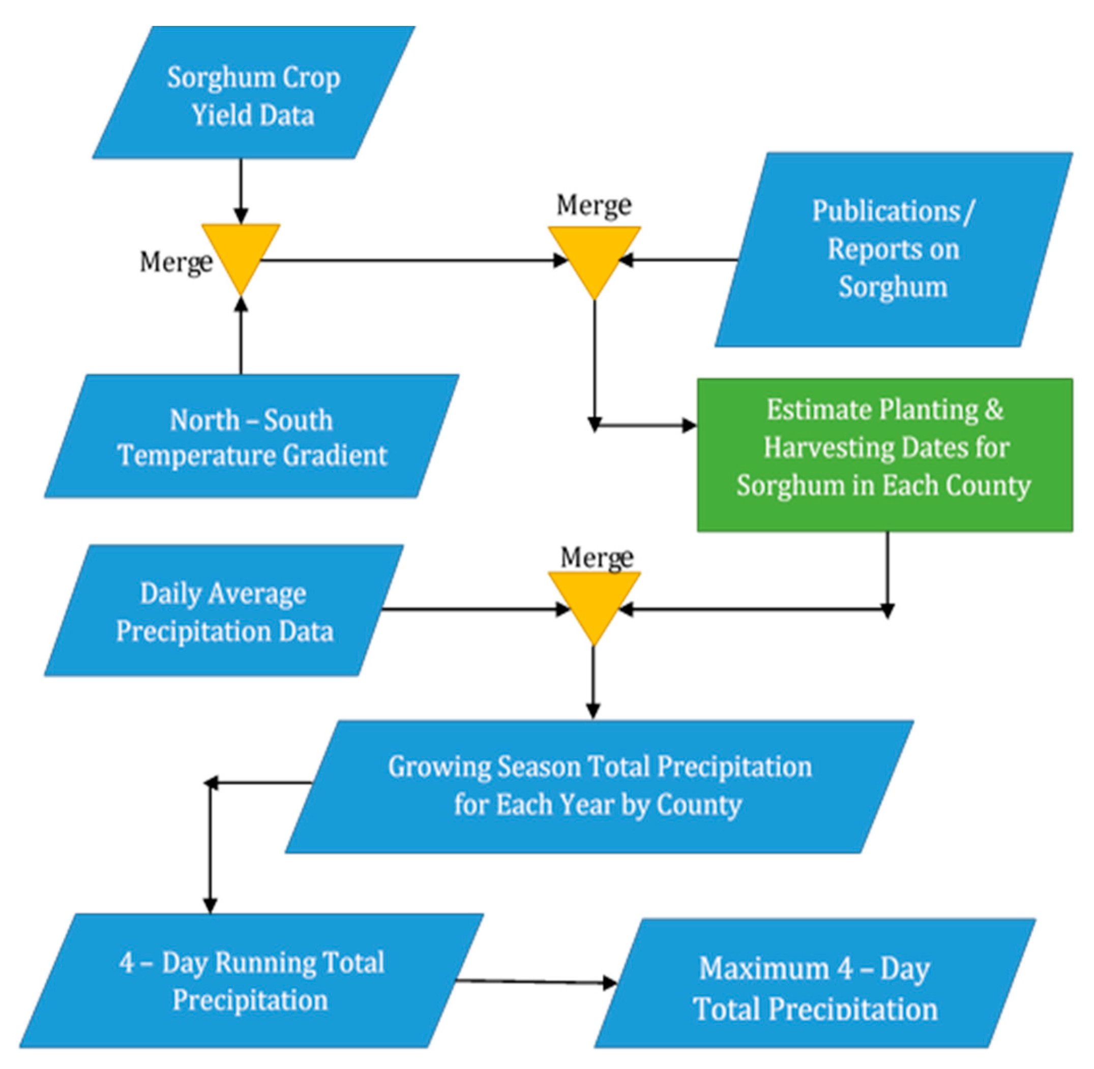
2.1.3. Estimation of Growing Season Precipitation by County
The growing season is the number of consecutive days from the beginning of planting date to the harvesting date. It is calculated for every county. To obtain the growing season total precipitation, the precipitation of all daily values within the growing season is added together. The precipitation data used for analysis for each county was taken from 10 days before the planting and harvesting dates of each station from the base date. This is because farmers would use soil moisture from any precipitation event before planting the seeds. Also, they harvest the crop only when the crop is adequately dry, avoiding days for harvest soon after precipitation (Figure 2).
2.1.4. Estimation of Maximum 4-Day Running Total Precipitation
The 4-day running total is the cumulative value of continuous four days of precipitation data. Continuous four days of precipitation is added to get one value, and so on. In this way, it is calculated for every day in the growing season for each year and station considered for the analysis. Finally, the maximum of four days of total precipitation within the grain sorghum growing season each year is calculated for every station for further graphical analysis.
2.2. Data Analysis
2.2.1. Level 1: Historically Documented Extreme Precipitation Events and Sorghum Yield in Texas
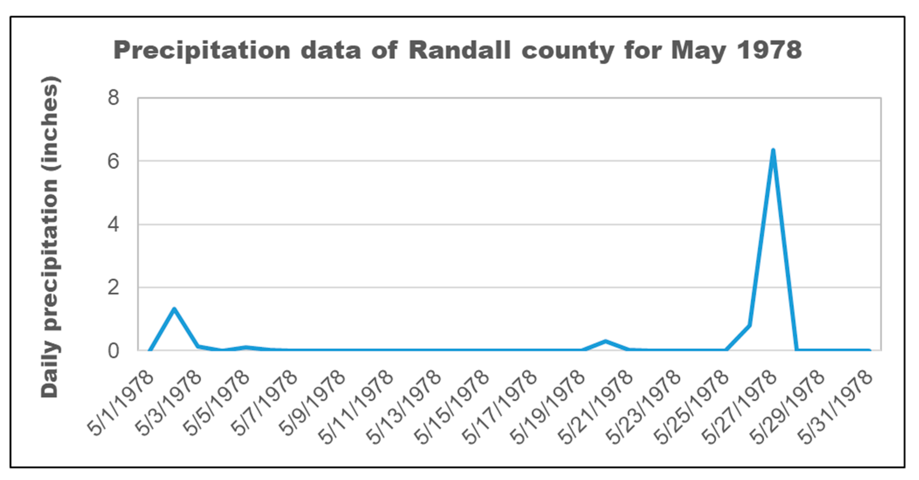
The High Plains and Low Rolling Plains climatic regions of Texas received an extreme rainfall of 508 mm (20 inches) over 26 km2 (10 square miles) area and 254 mm (10 inches) over 26,000 km2 (10 thousand square miles) from 1 August to 4 August in 1978. The East Texas and Upper Coast climatic regions of Texas received an extreme rainfall of 1000 mm (40 inches) for about 26 km2 (10 square miles) area and 254 mm (10 inches) for 26,000 km2 (10 thousand square miles) from 24 July to 28 July in 1979. Randall County had a storm during 26 May to 27 May 1978. The rainfall amount during the period averaged 100 mm to 254 mm (4 in. to 10 in.) on the High Plains. Out of all the extreme precipitation events documented, only the May 1978 storm in Randall County fell within the sorghum-growing season. Therefore, only the details of the May 1978 storm will be included for further analysis under this category [15,16].
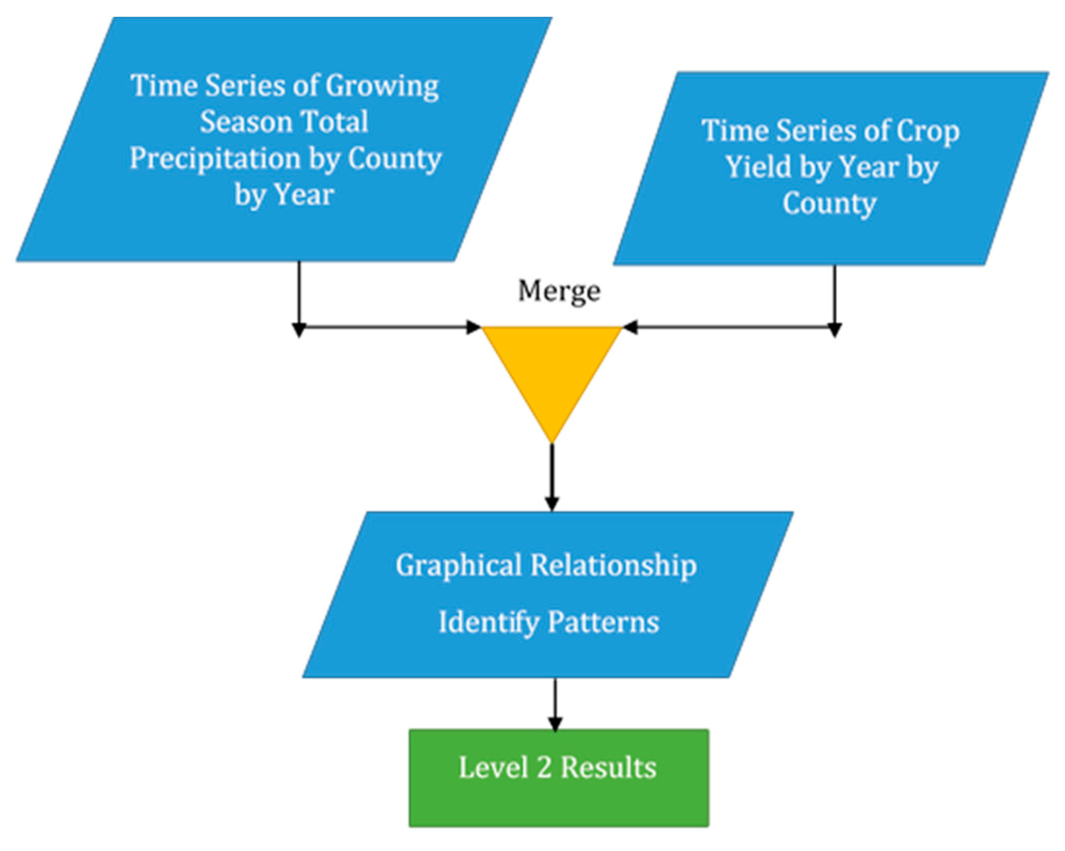
2.2.2. Level 2: Growing Season Precipitation and Rainfed Sorghum Crop Yields
The growing season’s total precipitation and rainfed sorghum crop yield for different years is plotted to identify graphical relationships (Figure A1). The trends in data for every county were analyzed.
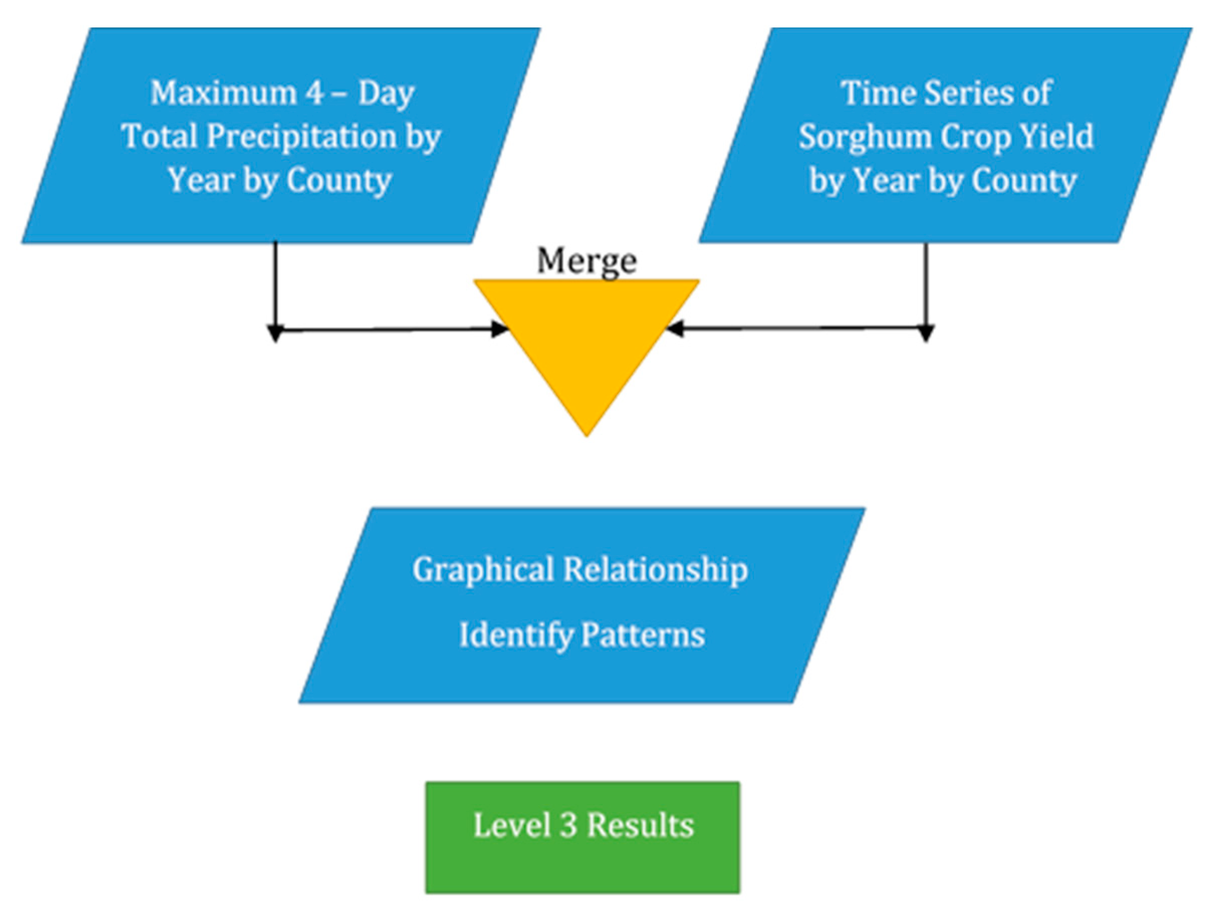
2.2.3. Level 3: Maximum 4-Day Running Total Precipitation and Crop Yield
The maximum 4-day running total precipitation and rainfed sorghum crop yield for different years is plotted to identify graphical relationships (Figure A2). The trends in data were studied for every county considered for the analysis.
2.2.4. Level 4: Generation of Mathematical Relationships between Rainfed Sorghum Yield and Excess Precipitation
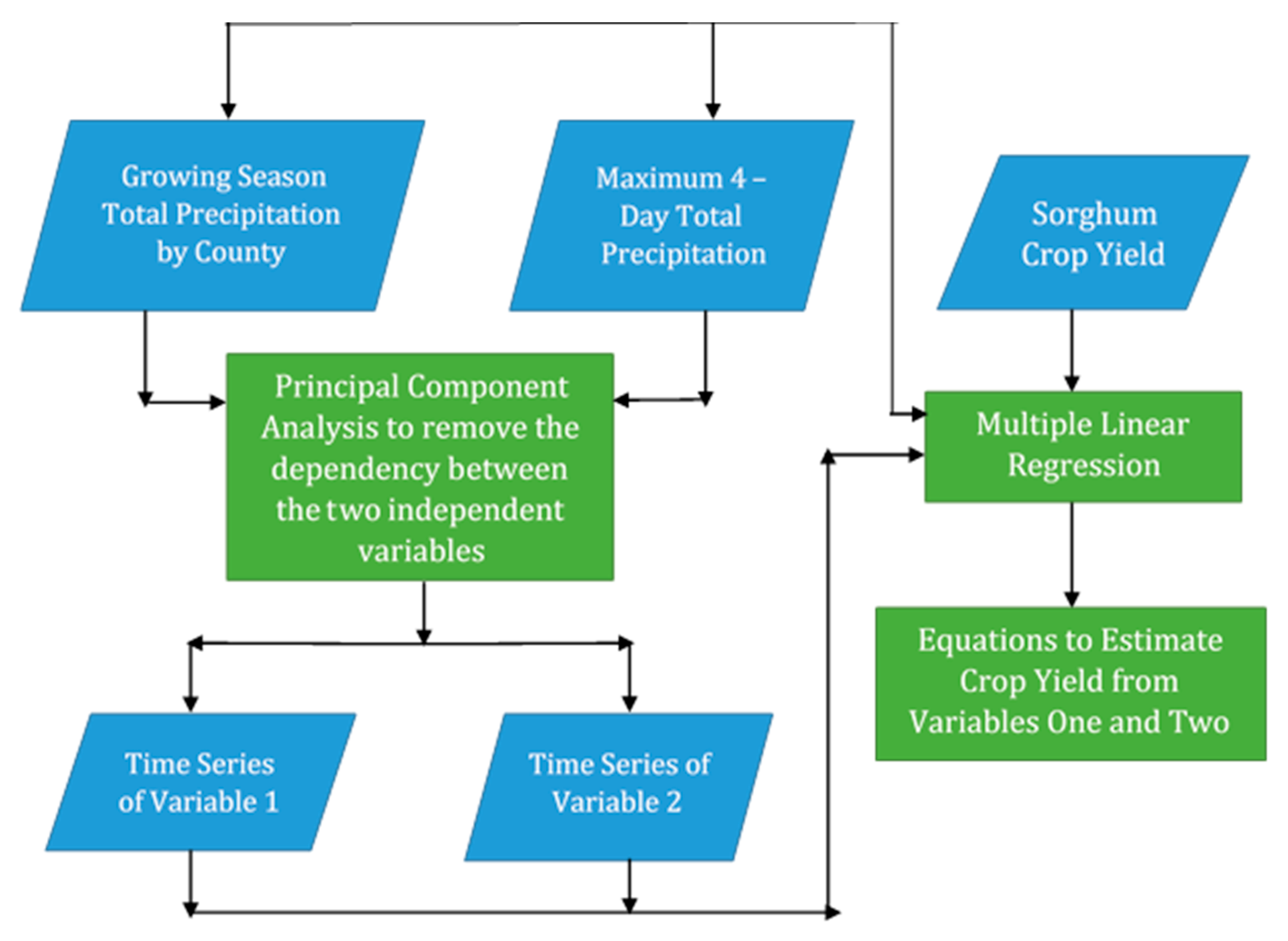
Principal component analysis (PCA) is a commonly used mathematical tool used to display patterns in multivariate data. It removes correlation within a large set of variables and sorts them according to importance (explained variance) [17]. While PCA is commonly used for dimensionality reduction, it was not used for that purpose in this study. Total precipitation and max 4-day precipitation are somewhat correlated, which could affect the regression relationships. PCA transforms the input variables to remove such correlation. A downside of PCA is that while the original variables have clear interpretations (total growing season precipitation and max 4-day precipitation), the PCA-transformed variables do not. They are called “principal components” 1 and 2.
In our regression analysis, the dependent variable was taken as the rainfed grain sorghum yield data, and the independent variables were growing season total precipitation and maximum 4-day total precipitation (Figure 3). Multiple linear regression (MLR) analysis (Equation (1)) [18] was performed with the data analysis tool available in Microsoft Excel.
where Y is crop yield, A is an intercept, X1 and X2 are growing season total precipitation and maximum 4-day total precipitation respectively, and B1 and B2 are partial regression coefficients [18].
Y = A + B1X1 + B2X2,
3. Results
3.1. Level 1 Results
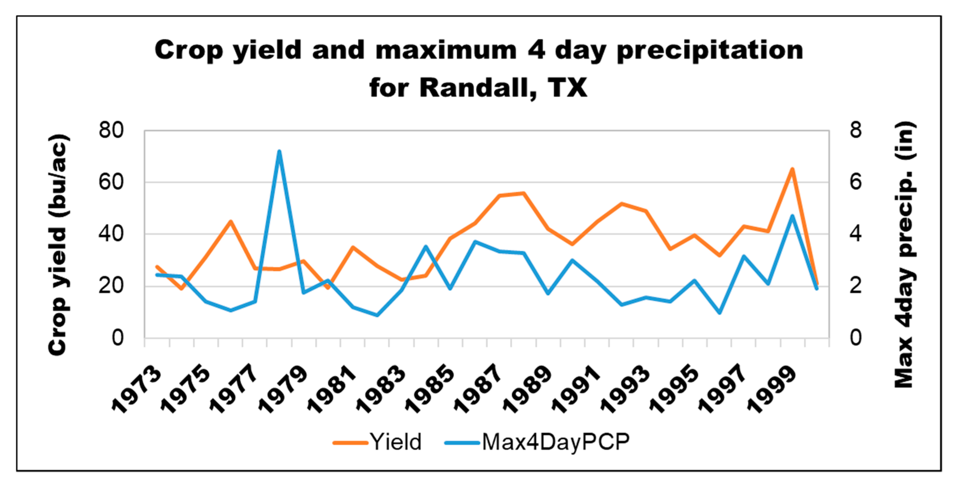
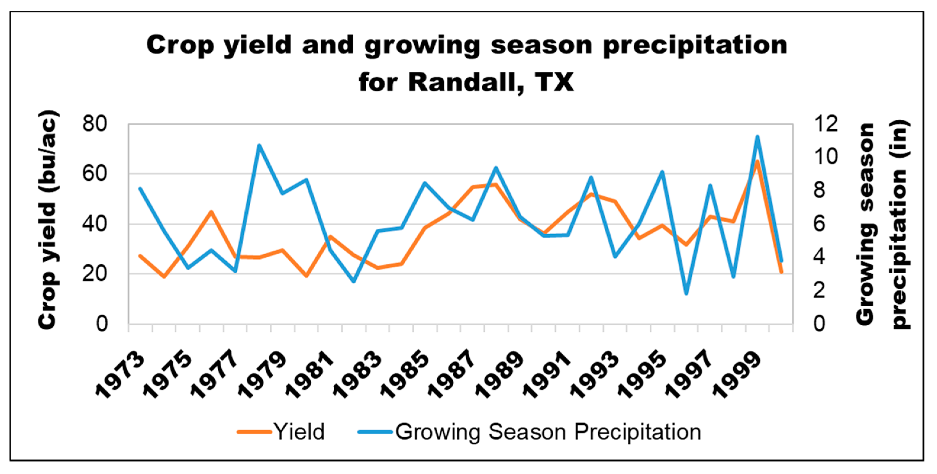
In the year 1978, Randall County encountered a storm event during the grain sorghum crop-growing period (26–27 May) (Figure 4). The 4-day maximum precipitation during the crop growing period was 182.9 mm (7.2 inches) which is 206% more than the average 4-day maximum precipitation (60.9 mm [2.4 inches]) that occurred during the sorghum crop growing period between 1973 and 2000. Also, the growing season total precipitation during the 1978 grain sorghum crop growing period was 271.8 mm (10.7 inches) which is 72.3% more than the average of the growing season total precipitation (157.5 mm (6.2 inches)) that occurred during the sorghum crop growing period between 1973 and 2000. The storm event could have brought down the rainfed sorghum yield by 27.5% (corresponding to the year 1978) when compared to the average rainfed sorghum yield from 1973 to 2000. This is evident from Figure 5 and Figure 6, which show the sharp declines in crop yields based on 4-day maximum precipitation and growing season total precipitation separately.
3.2. Level 2 Results
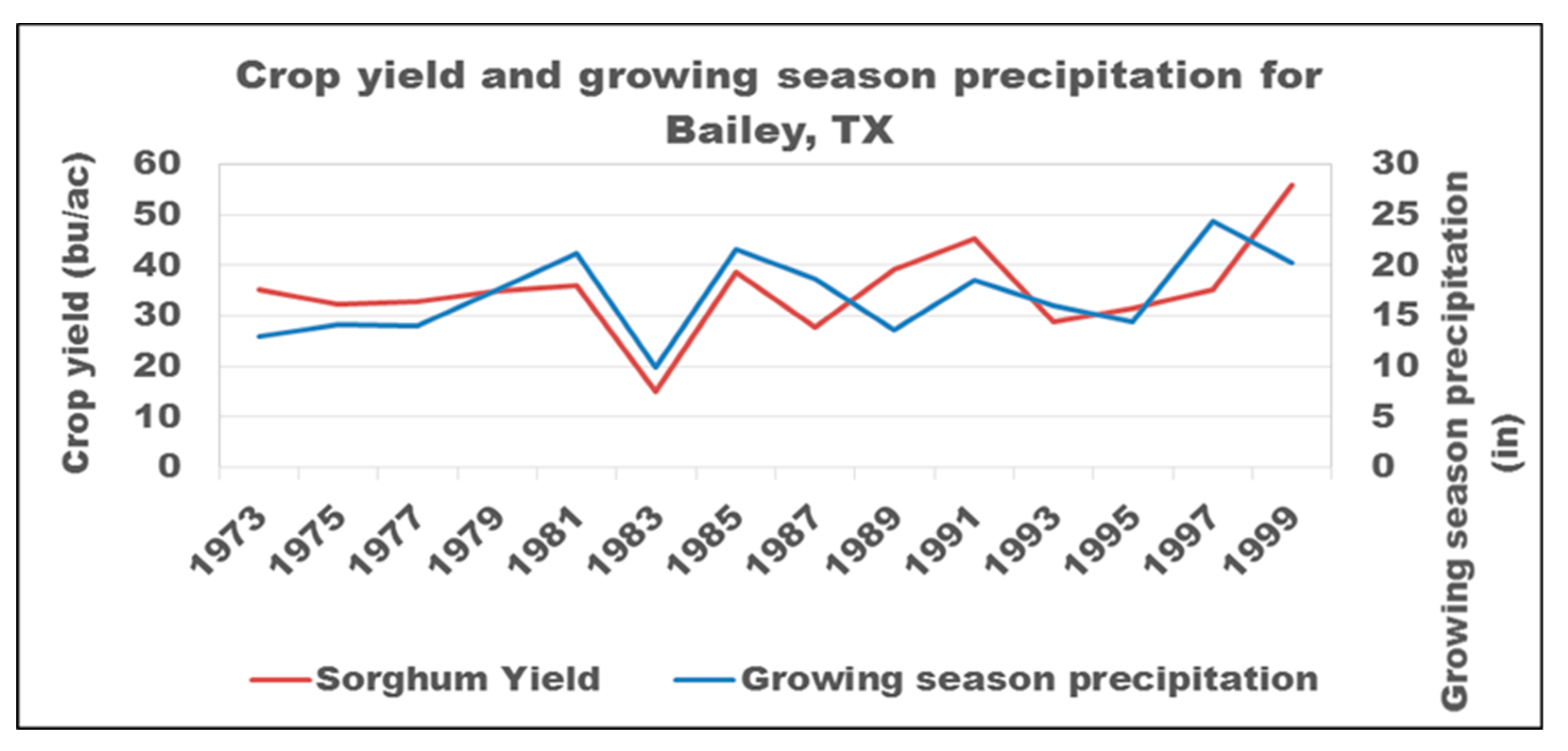
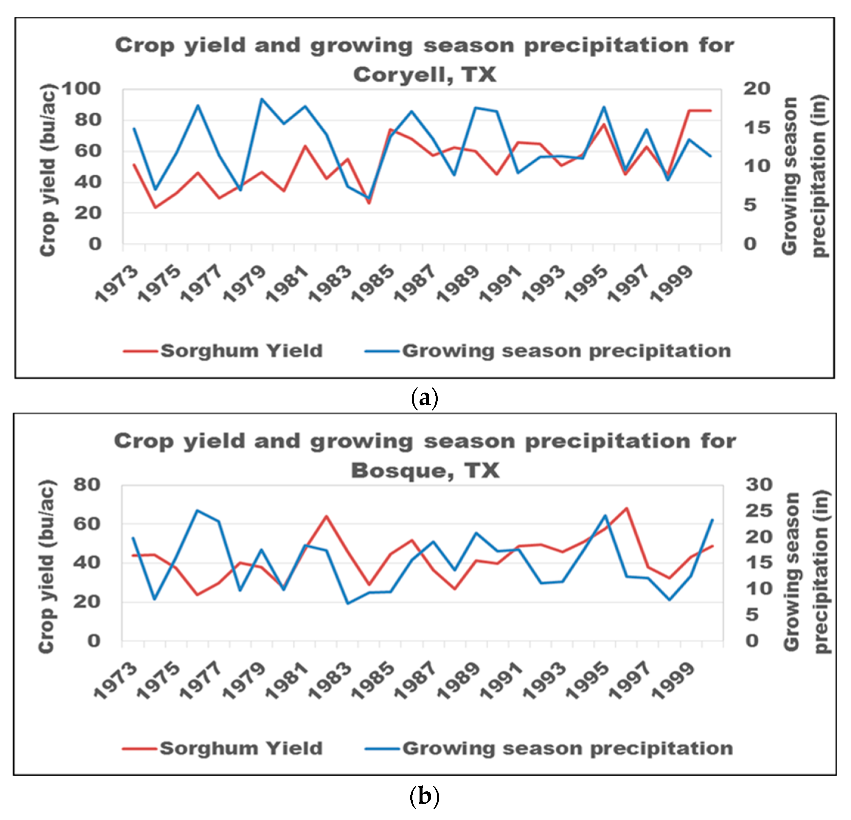
The graphical relationship between growing season total precipitation and rainfed sorghum crop yield was studied. Crop yield trends closely followed the growing season total precipitation for Texas counties Bailey, Bee, Cameron, Collin, Cooke, Dallam, Fannin, Hansford, Hunt, Jackson, and Wharton. When there was an increase in precipitation, there was a corresponding increase in the crop yield and vice versa (Figure 7). However, for some counties (e.g., Figure 8) there were declines in crop yield for excess precipitation. For Bosque County in 1976, growing season precipitation increased to 635 mm (25 inches) which resulted in a sharp decrease of crop yield. For Coryell County, when the annual growing season rainfall increased to 381 mm (15 inches) in 1976, it showed a decrease in crop yield. For Milam County in 1976, 1978, and 1994, increases in growing season total precipitation brought decreases in crop yield. Similar noticeable yield declines for excess precipitation results were observed for Atascosa, Gillespie, Hansford, Navarro, Randall, and Wise counties in Texas (Table 3) (graphs not shown in the manuscript for the sake of brevity).
The numerical analysis of crop yields and growing season total precipitation are provided in Table 3. When compared to the average for the period 1973 to 2000, the decreases in crop yield corresponding to the year(s) with excess precipitation is about 30% (95% confidence intervals 23% to 37%). When compared to the nearby years (before and after the year with excess precipitation), the years with excess precipitation showed a decrease in crop yield of 17% (95% confidence intervals 7% to 28%) (Table 3).
In summary, the analysis of numerical and graphical crop yield trends with respect to growing season total precipitation highlighted decreases in rainfed sorghum crop yield when the precipitation received is higher than the average or what could probably be necessary for healthy crop growth.
3.3. Level 3 Results
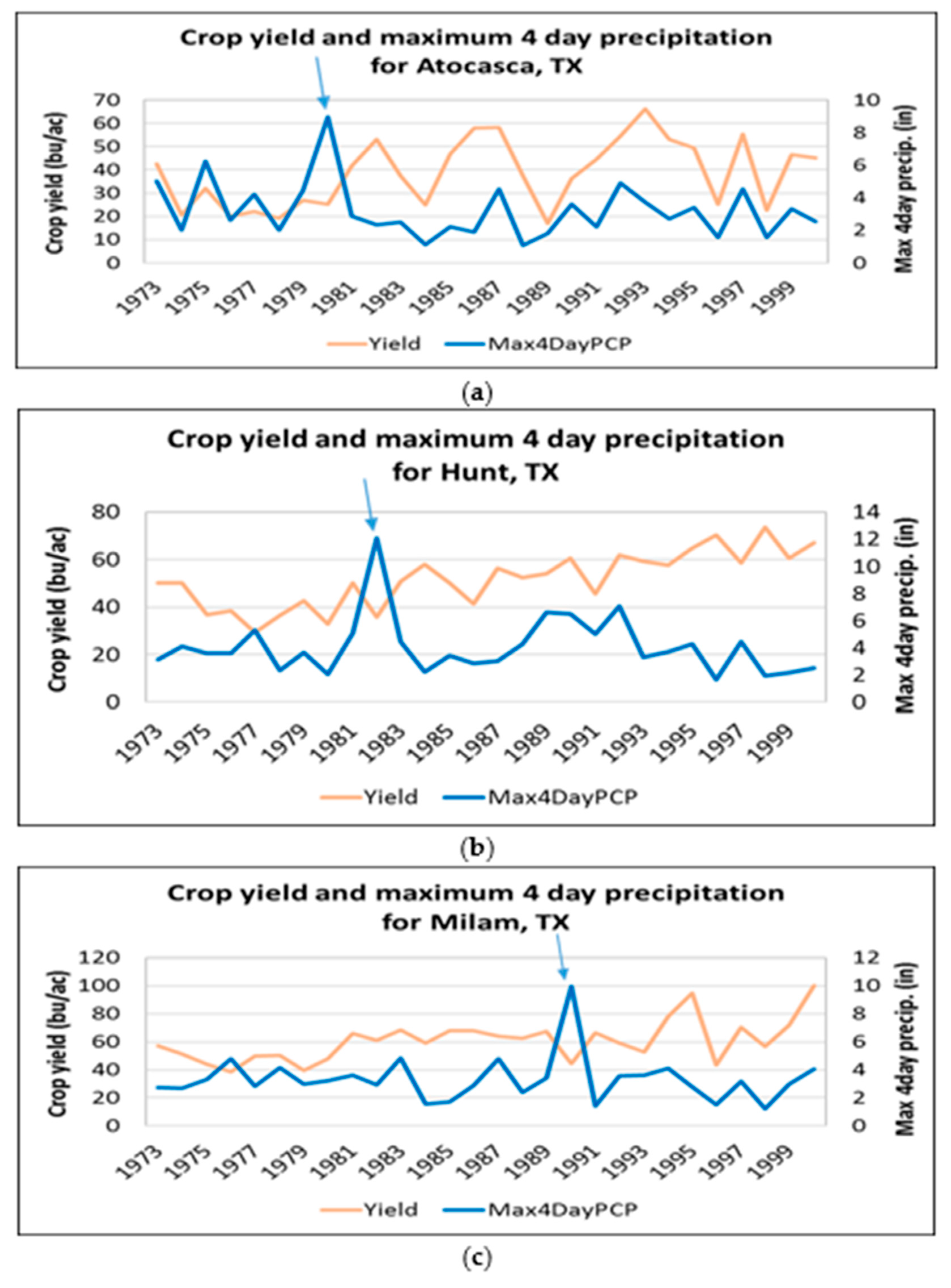
The graphical relationships of maximum 4-day total precipitation with rainfed sorghum crop yields were analyzed. Some of the results are shown in Figure 9. Crop yield trends closely follow the maximum 4-day total precipitation for Bailey, Bee, Bosque, Fannin, Dallam, Hale, Hunt, Jones, Matagorda, Nolan, and Wise counties. Atascosa County shows four days maximum total of 8 inches and results in the sharp decrease in crop yield for the year 1980 while for the other years the crop yield trends follow precipitation. For Hunt County, the four days precipitation go above 254 mm (10 inches) and result in a decrease in crop yield comparing to other years. The decrease in crop yield was observed for Milam County as well when the maximum 4-day total precipitation reached 254 mm (10 inches).
Similar rainfed sorghum yield declines were observed for high values of maximum 4-day running total precipitation for Coryell, Gillespie, Grey, Hansford, Matagorda, Navarro, Nolan, Randall, Wharton, and Wise counties. In summary, whenever the maximum four days running total precipitation is higher, that results in a decrease in crop yield of rainfed grain sorghum.
The numerical analysis of crop yields and maximum 4-day total precipitation are provided in Table 4. When compared to the average for the period 1973 to 2000 the decreases in crop yield corresponding to the year(s) with excess four-day precipitation is about 25% (95% confidence intervals 18% to 31%). When compared to the nearby years, the years with excess 4-day maximum precipitation showed a decrease in crop yield of 22% (95% confidence intervals 14% to 31%) (Table 4). In summary, the analysis of graphical and numerical crop yield trends with respect to maximum 4-day total precipitation pointed out decreases in rainfed sorghum crop yield when the precipitation received was much higher than the average or what could be necessary for healthy crop growth.
3.4. Level 4 Results
A multiple linear regression (MLR) analysis was performed with growing season total precipitation and maximum 4-day total precipitation as independent variables and rainfed sorghum yield as dependent variable the results of which are presented in Table 5. Although the R2 values (Column 5 of Table 5) appear smaller, the regression relationships are significant, as evidenced by the F values of regression relationships presented in Table 6. Looking at the regression relationships by county, negative coefficients appear for growing season total precipitation for counties Bosque, Dallam, Hansford, and Milam only. Twenty-three out of 27 counties analyzed mathematically did not show declines in crop yield for excess precipitation when analyzed by growing season total precipitation. However, when analyzed by the maximum 4-day total precipitation, 21 out of 27 counties show negative coefficients substantiating the declines in crop yield for excess precipitation. The counties that do not show negative coefficients (with maximum 4-day total precipitation) are Bee, Bosque, Dallam, Deaf Smith, Floyd, and Hansford. Majority of the counties analyzed mathematically exhibit declining crop yields for excess precipitation showing negative coefficients mostly in maximum 4-day total precipitation and some in growing season total precipitation. Milam is the only county showing a negative coefficient for both the independent variables. Although Deaf Smith and Floyd showed some graphical relationships, they were the only counties that did not mathematically exhibit the regression relationship between the independent variables and the dependent variable.
An MLR analysis like the one described above was performed with a PCA. The PCA was carried out to remove the relationship between the two independent variables. The results of the MLR are presented in Table 6; although the R2 values (Column 5 of Table 7) appear smaller, the regression relationships are significant as evidenced by the F values of regression relationships presented in Table 6. Looking at the regression relationships (with PCA) by county, negative coefficients appear for growing season total precipitation for Fannin, Hansford, Hunt, Jackson, and Milam counties only. Twenty-two out of 27 counties analyzed did not show declines in crop yield for excess precipitation when analyzed mathematically using regression relationships with growing season total precipitation and crop yields. However, when analyzed by the maximum 4-day total precipitation, 21 out of 27 counties show negative coefficients substantiating the declines in crop yield for excess precipitation. The counties that do not show negative coefficients are Bee, Bosque, Dallam, Deaf Smith, Floyd, and Hansford. Like the MLR without a PCA, most of the counties analyzed mathematically exhibit declining crop yields for excess precipitation showing negative coefficients mostly in maximum 4-day total precipitation and some in growing season total precipitation. Milam is the only county showing a negative coefficient for both the independent variables. Although showing some graphical relationships, Deaf Smith and Floyd are the only counties that did not mathematically exhibit the regression relationship between the independent variables and the dependent variable.
A comparison of the R2 values of regression relationships with and without PCA are presented in Table 8 which pointed out that the PCA did not offer a significant improvement in identifying relationships between excess precipitation and rainfed sorghum yield. However, there is some difference in the regression analysis results. In the regression without a PCA, only one county (Milam) did not mathematically show any declining crop yields with excess precipitation. In the regression with PCA, six out of 27 counties analyzed (Bee, Bosque, Dallam, Deaf Smith, Floyd, and Hansford) did not show declining crop yields with excess precipitation. However, the results analyzed in all four different levels point out the existence of crop yield declines with excess precipitation.
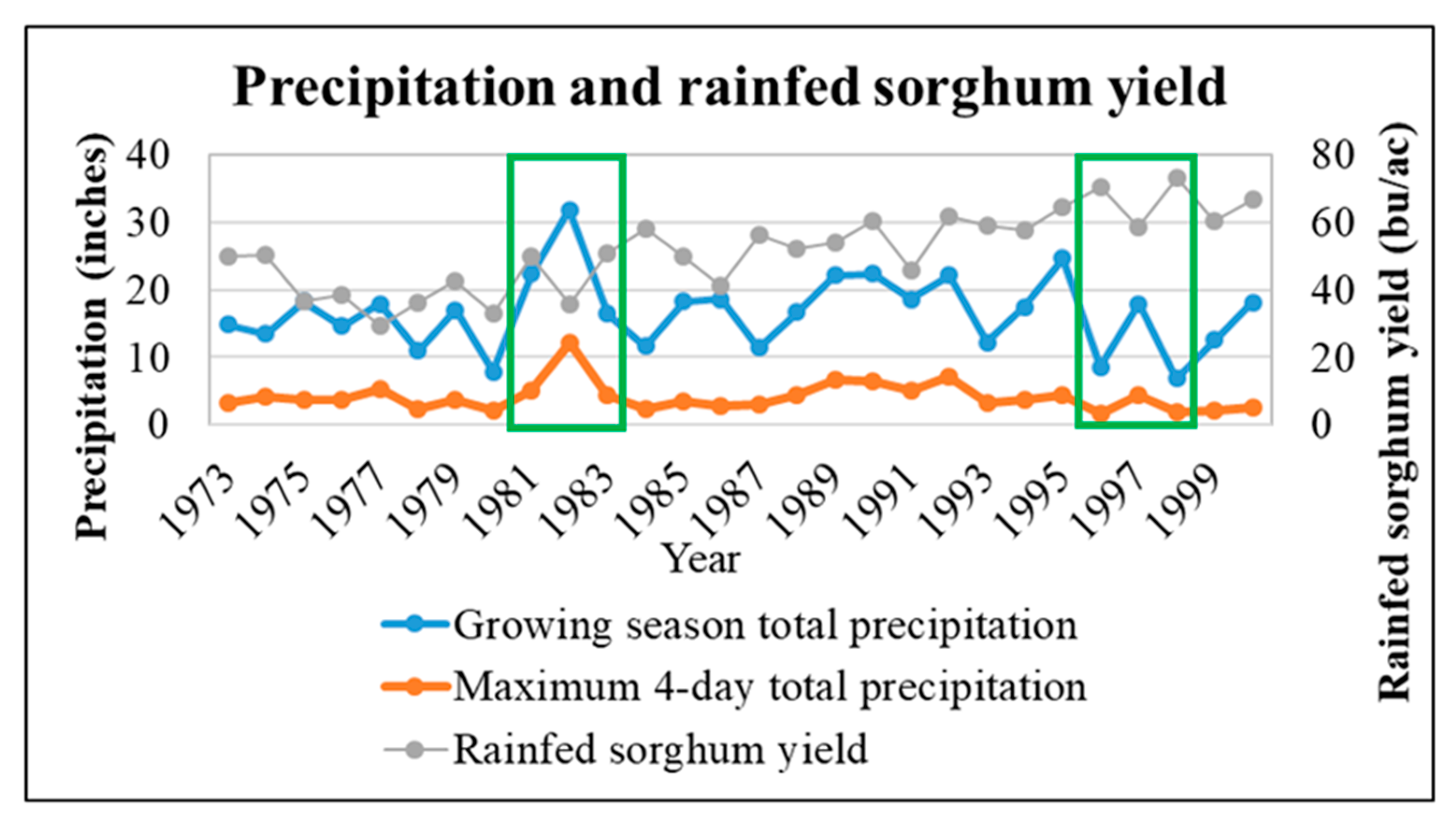
3.5. Substantiation of Crop Yield Declines with Excess Precipitation
In the previous section, the existence of crop yield decline with excess precipitation was identified based on separate graphical relationships between crop yield and growing season total precipitation, and crop yield and maximum 4-day total precipitation. The presence of crop yield decline for excess precipitation are substantiated by the graphical plot of crop yield, growing season total precipitation, and maximum 4-day total precipitation together for Hunt county in TX. The thin green rectangle outlined in Figure 10 identifies the hotspots that substantiate our findings described in the previous section(s).
3.6. Spatial Variation of Declines in Crop Yield for Excess Precipitation
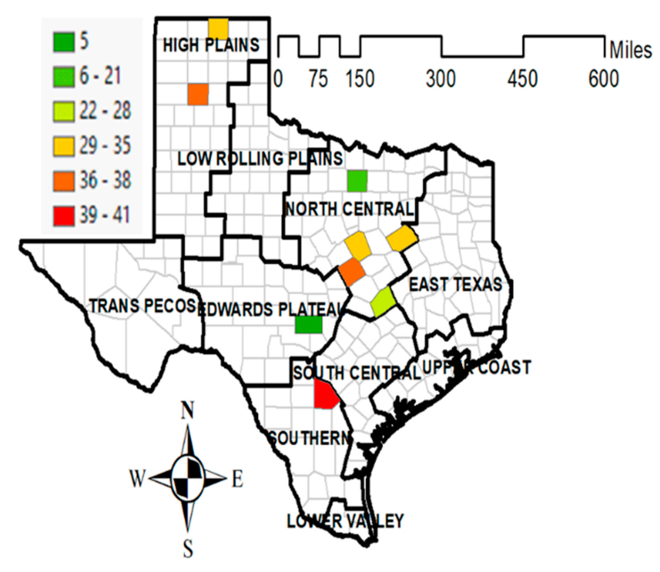
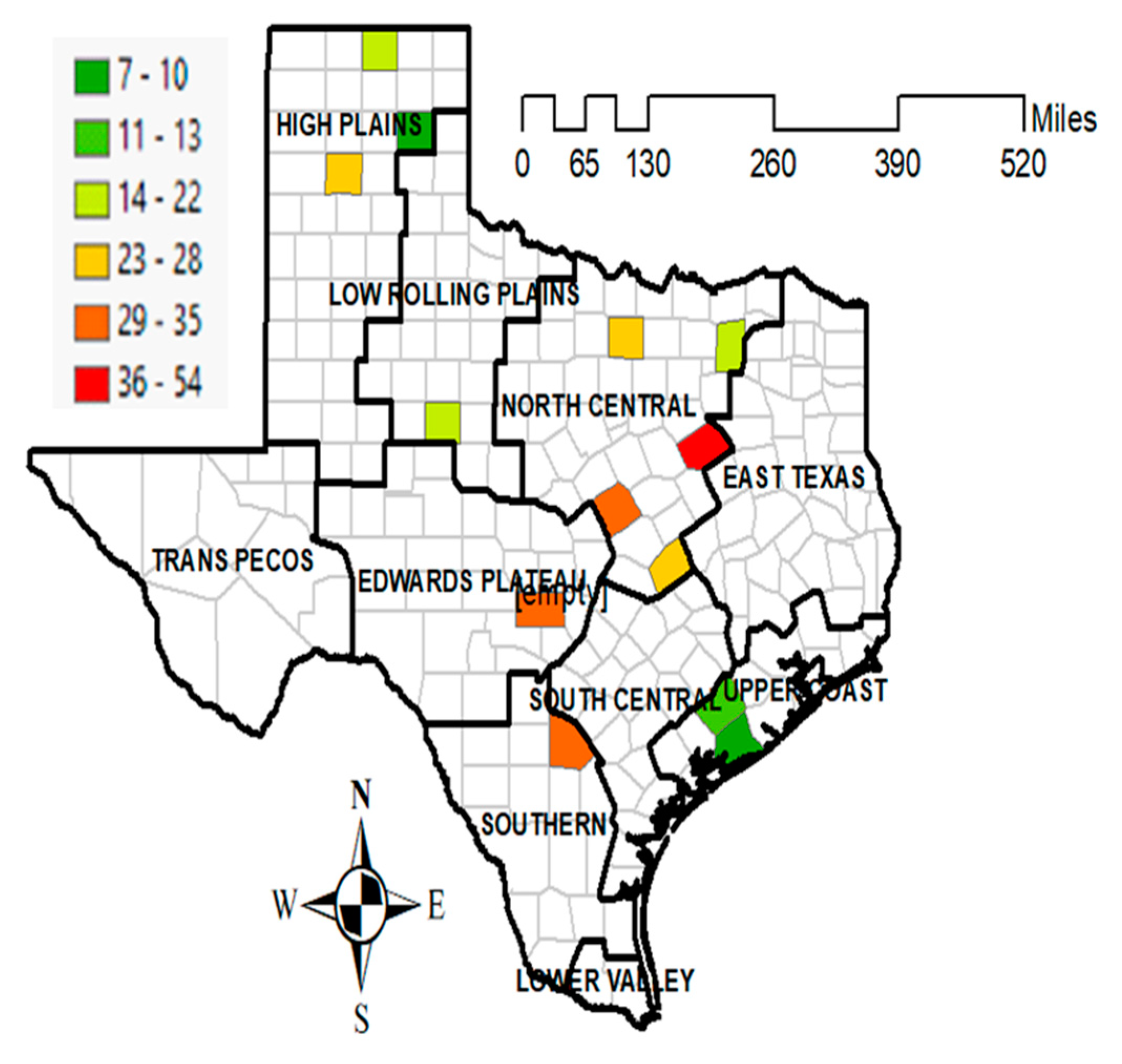
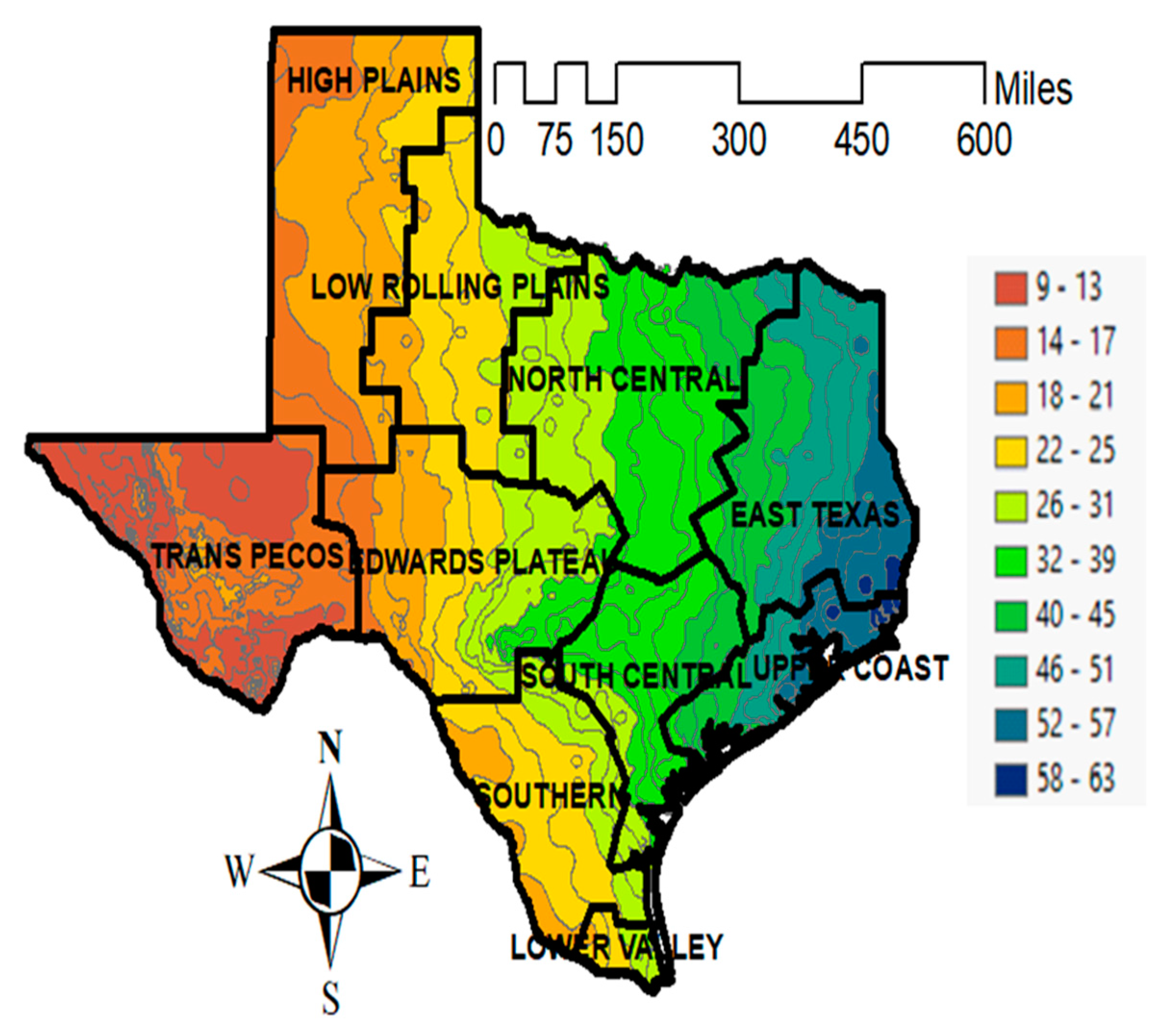
Counties and climate regions in Figure 11 and Figure 12, respectively show the spatial variation of declines in yield of sorghum for excess precipitation. Based on both growing season total precipitation and maximum 4-day total precipitation, the North Central region of Texas appears to be more vulnerable to rainfed sorghum yield declines than other parts of Texas. The other regions showing some crop yield decline for excess precipitation are the High Plains and Southern regions. The large variation of precipitation within the region (Figure 13) and precipitation patterns appear to be the probable reason that can be attributed. However, we need more evidence to substantiate this finding.
4. Discussion
For estimating crop yield losses, our study considered the quantity of precipitation alone leaving out another important aspect of precipitation, the timing with respect to the sorghum-growing season. In addition to excess precipitation, there are other contributing factors to yield losses such as high/low temperature (higher than optimum temperature for crop growth and lower than the crop base temperature), wind speed (high winds can dislodge the crop), humidity levels (excess would cause fungal problems), quality of soil (pH, drainage characteristics, depth), human decisions (e.g., whether or not going for pesticide application, irrigation, etc.), human errors in timing of land management operations (fertilizer or pesticide application, tillage, irrigation, and harvest). Therefore, care should be taken when interpreting the results of our study.
In addition to the approach used in this study, there are other ways of estimating crop yield losses by excess precipitation. The possibility of using remote sensing techniques to estimate crop yield losses by flooding was explored in Tapia-Silva et al. [20] using the August 2002 flooding event in Germany. In their approach, the flood crop loss is a function of crop value and a damage factor. The damage factor is a function of type of crop, timing of flood event, and inundation duration. When compared to field observations, they were able to estimate the crop losses with limited success. Their analysis dealt with flood inundation area of cropped fields rather than the proportion of yield loss.
There were a few other studies that explored the relationship between excess precipitation and crop yield reductions. Rosenzweig et al. [21] documented the extreme weather events that occurred in the US between 1977 and 1998; many of them include severe flooding events that resulted in reductions in crop yield. Increased moisture resulting from excess precipitation helps to spread epidemics and prevalence of leaf fungal pathogens, for example, fungal epidemics in corn, soybean, alfalfa, and wheat reported to have occurred in the US Midwest in 1993. The same period also saw incidences of soybean sudden death and mycotoxin increases [21]. Continuous soil saturation causing crazy top and common smut are also documented in the same study.
Corn yield reductions due to excess soil moisture (resulting from high precipitation) during current conditions and future conditions (under climate change) were estimated by Rosenzweig et al. [9] using CERES-maize model for the US Midwest. The current conditions showed a 3% reduction in corn yield ($600 million for the US corn production) because of aeration stress resulting from excess precipitation in the US Midwest. However, they have also estimated the increase in frequency of excess precipitation events in the future because of climate change. The same study also points out that when compared to the present, 90% more decreases in crop yield losses by 2030 and 150% more yield losses are expected by 2090. Winter wheat yield response to many parameters were analyzed in the Netherlands including excess precipitation. Except for one precipitation event in week 31 of the calendar year, they could not find any noticeable yield reductions for winter wheat resulting from excess precipitation [22].
The topic discussed in this manuscript relates to the idea of water use efficiency and water footprint. Water-use efficiency [23] is the ratio of aboveground biomass production to the water evapotranspired. The biomass is usually determined as dry weight rather than as fresh weight because moisture content of crops is different, which can mislead the interpretation of the water-use efficiency results. The results are usually expressed in kg L−1 or t m−3. In the context of water-use efficiency, the reductions in crop yield during excess precipitation will present a less water efficient scenario. Therefore, care should be taken when interpreting the water-use efficiency results.
Water footprint [24,25] is the inverse of the water-use efficiency described above. The typical units are L kg−1 (L of water required to produce a kg of useful yield) or m3 t−1 (m3 of water required to produce a metric ton of useful yield). Green water footprint is water from precipitation that is stored in the root zone of the soil and evaporated, transpired, or incorporated by plants [24]. For rainfed crops, the inverse of water-use efficiency is analogous to green water footprint. The reductions in crop yield during excess precipitation will produce a relatively large green water footprint. Therefore, care should be taken when interpreting the water footprint results for crops that underwent an excess precipitation scenario like what is discussed in our study. The simplest way to avoid misleading water-use efficiency and green water footprint results are to use the average values from multiple crop growing years capturing a range of climatic scenarios.
The results of this study and other similar studies have applications in payment of crop insurance claims, parameterization of computer models (estimating crop yield reductions based on aeration stress), policy level decisions on rainfed crop selection, yield forecasting, estimating threats to food production, and water footprint analysis.
5. Conclusions
We collected historical crop yield data for Texas by county for grain sorghum from 1973 to 2000 and the corresponding daily precipitation data from weather stations within the counties. After estimating the crop growing season for sorghum in different parts of Texas, we estimated the growing season total precipitation and maximum 4-day total precipitation for each county growing rainfed grain sorghum. Using the two parameters mentioned above as independent variables, and crop yield of sorghum as the dependent variable, we tried to find out relationships between excess precipitation and decreases in crop yields using both graphical and mathematical relationships. We carried out a multiple linear regression (MLR) analysis with and without the use of a principal component analysis (PCA). Based on the results obtained, we can conclude that:
- Excess precipitation during crop growing season can cause yield reduction in rainfed grain sorghum.
- Total precipitation during the growing season and maximum 4-day total precipitation during the growing season are potential indicators of yield reductions in grain sorghum.
- Yield reductions could be in the range of 18% to 38% for rainfed grain sorghum in Texas because of excess precipitation during the growing season.
- When analyzed spatially, the north-central climate region of Texas appears to be more vulnerable to rainfed sorghum yield reductions because of excess precipitation.
Author Contributions
O.P.S. carried out most parts of the study. N.K. conceptualized the overall study, S.C. designed and carried out the principal component analysis; regression analysis was carried out by O.P.S. under the supervision of S.C. and N.K. B.K.P. analyzed the results of the study. Most of the GIS analysis was carried out by C.M. All the authors contributed to the development of this manuscript.
Funding
Funding for this study is provided by Tarleton State University under the Faculty-Student Research and Creative Activity Internal Grants.
Acknowledgments
The authors acknowledge Tarleton State University for supporting this research.
Conflicts of Interest
As the guest editor of the special issue “Water Management for Sustainable Food Production”, Narayanan Kannan has a conflict of interest. Therefore, the assistant editors, and the editor-in-chief (of Water-MDPI), were involved in inviting reviewers, analyzing the peer review report and making the decision on acceptance of the article for publication.
Appendix A

Table A1.
List of counties in Texas that have rainfed sorghum yield data is available.
| Station Number | County | Latitude | Longitude |
|---|---|---|---|
| 2 | Atascosa | 28.92 | −98.74 |
| 4 | Bailey | 34.21 | −102.73 |
| 6 | Bee | 28.45 | −97.70 |
| 9 | Bosque | 32.01 | −97.61 |
| 16 | Cameron | 25.91 | −97.42 |
| 20 | Collin | 33.03 | −96.48 |
| 23 | Cooke | 33.48 | −97.15 |
| 24 | Coryell | 31.27 | −97.88 |
| 26 | Dallam | 36.23 | −102.24 |
| 28 | Deaf Smith | 34.93 | −102.98 |
| 36 | Fannin | 33.43 | −96.33 |
| 39 | Floyd | 33.98 | −101.33 |
| 41 | Gillespie | 30.18 | −99.15 |
| 42 | Gray | 35.55 | −100.97 |
| 43 | Hale | 34.18 | −101.7 |
| 45 | Hansford | 36.19 | −101.18 |
| 46 | Hunt | 33.36 | −96.06 |
| 47 | Jackson | 28.96 | −96.68 |
| 48 | Jones | 32.94 | −99.8 |
| 50 | Matagorda | 28.68 | −95.97 |
| 52 | Milam | 30.61 | −97.2 |
| 53 | Navarro | 31.96 | −96.68 |
| 54 | Nolan | 32.44 | −100.52 |
| 58 | Randall | 34.95 | −102.1 |
| 66 | Wharton | 29.31 | −96.08 |
| 67 | Wise | 33.35 | −97.39 |
Figure A1.
Generation of the graphical relationship between rainfed sorghum yield and growing season total precipitation (level 2 results).
Figure A1.
Generation of the graphical relationship between rainfed sorghum yield and growing season total precipitation (level 2 results).

Figure A2.
Generation of the graphical relationship between rainfed sorghum yield and maximum 4–day total precipitation (level 3 results).
Figure A2.
Generation of the graphical relationship between rainfed sorghum yield and maximum 4–day total precipitation (level 3 results).

References
- Tsuchihashi, N.; Goto, Y. Year-round cultivation of sweet sorghum [Sorghum bicolor (L.) Moench] through a combination of seed and ratoon cropping in Indonesian Savanna. Plant Prod. Sci. 2008, 11, 377–384. [Google Scholar] [CrossRef]
- Sorghum Program. Available online: https://www.sorghumcheckoff.com/all-about-sorghum (accessed on 31 July 2019).
- Eggen, M.; Ozdogan, M.; Zaitchik, B.; Ademe, D.; Foltze, J.; Simane, B. Vulnerability of sorghum production to extreme, sub-seasonal weather under climate change. Environ. Res. Lett. 2019, 14, 045005. [Google Scholar] [CrossRef]
- New, L. Grain Sorghum Irrigation; Texas A&M AgriLife Extension: Amarillo, TX, USA, 2004.
- Arkansas Sorghum Quick Facts. Available online: https://www.uaex.edu/farm-ranch/crops-commercial-horticulture/grain-sorghum/2014-Arkansas-Grain-Sorghum-Quick-Facts.pdf (accessed on 31 July 2019).
- Promkhambut, A.; Younger, A.; Polthanee, A.; Akkasaeng, C. Morphological and physiological responses of Sorghum (Sorghum bicolor L. Moench) to Waterlogging. Asian J. Plant Sci. 2010, 9, 183–193. [Google Scholar]
- Lobell, D.; Burke, M.B.; Tebaldi, C.; Mastrandrea, M.D.; Falcon, W.P.; Naylor, R.L. Prioritizing climate change adaptation needs for food security in 2030. Science 2008, 319, 607–610. [Google Scholar] [CrossRef] [PubMed]
- Grossi, M.C.; Justino, F.; Rodrigues, R.; Andrade, C.L.T. Sensitivity of the sorghum yield to individual changes in climate parameters: Modelling based approach. Bragantia 2015, 74, 341–349. [Google Scholar] [CrossRef]
- Rosenzweig, C.; Tubiello, F.N.; Goldberg, R.; Mills, E.; Bloomfield, J. Increased crop damage in the US from excess precipitation under climate change. Glob. Environ. Chang. 2002, 12, 197–202. [Google Scholar] [CrossRef] [Green Version]
- Balling, R.C., Jr.; Goodrich, G.B. Spatial analysis of variations in precipitation intensity in the USA. Theor. Appl. Climatol. 2011, 104, 415–421. [Google Scholar] [CrossRef]
- Kunkel, K.E.; Karl, T.R.; Brooks, H.; Kossin, J.; Lawrimore, J.H.; Arndt, D.; Bosart, L.; Changnon, D.; Cutter, S.L.; Doesken, N.; et al. Monitoring and understanding trends in extreme storms: State of knowledge. Bull. Am. Meteorol. Soc. 2013, 94, 499–514. [Google Scholar] [CrossRef]
- Texas Natural Resources Information Systems (TNRIS). Available online: https://data.tnris.org/ (accessed on 31 July 2019).
- Jin, S.; Yang, L.; Danielson, P.; Homer, C.; Fry, J.; Xian, G. A comprehensive change detection method for updating the National Land Cover Database to circa 2011. Remote Sens. Environ. 2013, 132, 159–175. [Google Scholar] [CrossRef] [Green Version]
- United States Department of Agriculture-National Agricultural Statistical Service (USDA-NASS). Field Crops Usual Planting and Harvesting Dates; Agricultural Handbook Number 626; USDA-NASS: Washington, DC, USA, 2010.
- Mishra, A.K.; Singh, V.P. Changes in extreme precipitation in Texas. J. Geophys. Res. Atmos. 2010, 115. [Google Scholar] [CrossRef]
- Nielsen-Gammon, J.W.; Zhang, F.; Odins, A.M.; Myoung, B. Extreme rainfall in Texas: Patterns and predictability. Phys. Geogr. 2005, 26, 340–364. [Google Scholar] [CrossRef]
- Jolliffe, I.T. Principal Component Analysis, 2nd ed.; Springer: New York, NJ, USA, 2002. [Google Scholar]
- Bluman, A.G. Elementary Statistics: A Step by Step Approach, 7th ed.; McGraw Hill Publishers: New York, NJ, USA, 2009. [Google Scholar]
- Texas Water Development Board (TWDB). GIS Data. Available online: www.twdb.texas.gov/mapping/gisdata.asp (accessed on 10 June 2019).
- Tapia-Silva, F.; Itzerott, S.; Foerster, S.; Kuhlmann, B.; Breibich, H. Estimation of flood losses to agricultural crops using remote sensing. Phys. Chem. Earth 2011, 36, 253–265. [Google Scholar] [CrossRef]
- Rosenzweig, C.; Iglesias, A.; Yang, X.B.; Epstein, P.R.; Chivian, E. Climate change and extreme weather events Implications for food production, plant diseases, and pests. Glob. Chang. Hum. Health 2001, 2, 90–104. [Google Scholar] [CrossRef]
- Powell, J.P.; Reinhard, S. Measuring the effects of extreme weather events on yields. Weather Clim. Extremes 2016, 12, 69–79. [Google Scholar] [CrossRef] [Green Version]
- Kirkham, M.B. Water use efficiency. In Encyclopedia of Soils in the Environment, Reference module in Earth Systems and Environmental Sciences; Elsevier: Cambridge, MA, USA, 2005; pp. 315–322. [Google Scholar]
- Hoekstra, A.Y. The Water Footprint of Modern Consumer Society; Routledge: London, UK, 2013. [Google Scholar]
- Zhang, Y.; Huang, K.; Yu, Y.; Yang, B. Mapping of water footprint research: A bibliometric analysis during 2006–2015. J. Clean. Prod. 2017, 149, 70–79. [Google Scholar] [CrossRef]
Figure 1.
Map showing the location of Meteorological stations and rainfed sorghum cultivated location.
Figure 1.
Map showing the location of Meteorological stations and rainfed sorghum cultivated location.

Figure 2.
Estimation of growing season total precipitation and maximum 4-day total precipitation.

Figure 3.
Schematic for the multiple linear regression (MLR) with and without a principal component analysis (PCA) (level 4 results).
Figure 3.
Schematic for the multiple linear regression (MLR) with and without a principal component analysis (PCA) (level 4 results).

Figure 4.
Storm event of May 1978 in Randall County.

Figure 5.
Sorghum yield reductions for Randall County in 1978 coming from maximum 4-day total precipitation.
Figure 5.
Sorghum yield reductions for Randall County in 1978 coming from maximum 4-day total precipitation.

Figure 6.
Sorghum yield reductions for Randall County in 1978 coming from excess growing season precipitation.
Figure 6.
Sorghum yield reductions for Randall County in 1978 coming from excess growing season precipitation.

Figure 7.
Example for crop yield trends closely following growing season total precipitation.

Figure 8.
Relationship between growing season precipitation and crop yield for (a) Coryell County, (b) Bosque County, and (c) Milam County.
Figure 8.
Relationship between growing season precipitation and crop yield for (a) Coryell County, (b) Bosque County, and (c) Milam County.


Figure 9.
Relationship between maximum 4-day total precipitation and rainfed sorghum yield for (a) Atascosa (b) Hunt, and (c) Milam counties.
Figure 9.
Relationship between maximum 4-day total precipitation and rainfed sorghum yield for (a) Atascosa (b) Hunt, and (c) Milam counties.

Figure 10.
Graph showing rainfed sorghum yield, maximum 4-day total precipitation, and growing season total precipitation for Hunt County.
Figure 10.
Graph showing rainfed sorghum yield, maximum 4-day total precipitation, and growing season total precipitation for Hunt County.

Figure 11.
Percent reduction in rainfed sorghum yield between the year with excess precipitation and average crop yield from 1973 to 2000 (based on growing season total precipitation).
Figure 11.
Percent reduction in rainfed sorghum yield between the year with excess precipitation and average crop yield from 1973 to 2000 (based on growing season total precipitation).

Figure 12.
Percent reduction in rainfed sorghum yield between the year with excess precipitation and average crop yield from 1973 to 2000 (based on maximum 4-day total precipitation).
Figure 12.
Percent reduction in rainfed sorghum yield between the year with excess precipitation and average crop yield from 1973 to 2000 (based on maximum 4-day total precipitation).

Figure 13.
Variation of precipitation in different climate regions of Texas [19].
Figure 13.
Variation of precipitation in different climate regions of Texas [19].

Table 1.
Estimated grain sorghum water use by growth stage [5].
Table 1.
Estimated grain sorghum water use by growth stage [5].
| Days after Sorghum Planting | Water Requirement (Inches/Day) | Water Requirement (mm/day) |
|---|---|---|
| 0–30 (early plant growth) | 0.05–0.10 | 1.3–2.5 |
| 30–60 (rapid plant growth) | 0.10–0.20 | 2.5–5.0 |
| 60–80 (boot and flowering) | 0.25–0.30 | 6.3–7.5 |
| 80–120 (grain fill to maturity) | 0.10–0.25 | 2.5–6.3 |
Table 2.
Plant date of sorghum in different counties of Texas [14].
Table 2.
Plant date of sorghum in different counties of Texas [14].
| County | Planting Date | Harvest Date | Precipitation Start | Precipitation End | ||
|---|---|---|---|---|---|---|
| Early | Late | Used | ||||
| Atascosa | 3/10–3/15 | 3/15–3/25 | 15-March | 3-July | 5-March | 25-June |
| Bailey | 3/5–3/10 | 3/10–3/20 | 10-March | 28-June | 1-March | 18-June |
| Bee | 1/21–1/30 | 1/31–2/10 | 30-January | 20-May | 20-Jan | 10-May |
| Bosque | 3/15–3/25 | 3/26–4/5 | 25-March | 13-July | 15-March | 3-July |
| Cameron | 1/21–1/30 | 1/31–2/10 | 30-January | 20-May | 20-Jan | 10-May |
| Collin | 3/25–4/4 | 4/5–4/15 | 4-April | 23-July | 26-March | 13-July |
| Cooke | 3/15–3/25 | 3/26–4/5 | 25-March | 13-July | 15-March | 3-July |
| Coryell | 3/15–3/25 | 3/25–4/5 | 25-March | 13-July | 15-March | 3-July |
| Dallam | 3/5–3/10 | 3/10–3/20 | 10-March | 28-June | 1-March | 18-June |
| Fannin | 3/25–4/4 | 4/5–4/15 | 4-April | 23-July | 26-March | 13-July |
| Floyd | 3/5–3/10 | 3/10–3/20 | 10-March | 28-June | 1-March | 18-June |
| Gillespie | 3/10–3/15 | 3/15–3/25 | 15-March | 3-July | 5-March | 25-June |
| Gray | 3/5–3/10 | 3/10–3/20 | 10-March | 28-June | 1-March | 18-June |
| Hale | 3/5–3/10 | 3/10–3/20 | 10-March | 28-June | 1-March | 18-June |
| Hansford | 3/5–3/10 | 3/10–3/20 | 10-March | 28-June | 1-March | 18-June |
| Hunt | 3/25–4/4 | 4/5–4/15 | 4-April | 23-July | 26-March | 13-July |
| Jackson | 2/15–2/21 | 2/22–3/5 | 21-February | 11-June | 11-February | 1-June |
| Jones | 3/5–3/10 | 3/10–3/20 | 10-March | 28-June | 1-March | 18-June |
| Matagorda | 2/15–2/21 | 2/22–3/5 | 21-February | 11-June | 11-February | 1-June |
| Milam | 3/15–3/25 | 3/26–4/5 | 25-March | 13-July | 15-March | 3-July |
| Navarro | 3/25–4/4 | 4/5–4/15 | 4-April | 23-July | 26-March | 13-July |
| Nolan | 3/5–3/10 | 3/10–3/20 | 10-March | 28-June | 1-March | 18-June |
| Randall | 3/5–3/10 | 3/10–3/20 | 10-March | 28-June | 1-March | 18-June |
| Wharton | 2/15–2/21 | 2/22–3/5 | 21-February | 11-June | 11-February | 1-June |
| Wise | 3/15–3/25 | 3/26–4/5 | 25-March | 13-July | 15-March | 3-July |
Table 3.
Differences in sorghum yield between average growing season total precipitation (for years 1973–2000) and years showing high growing season total precipitation (column 2) and years nearby high growing season total precipitation (column 3).
Table 3.
Differences in sorghum yield between average growing season total precipitation (for years 1973–2000) and years showing high growing season total precipitation (column 2) and years nearby high growing season total precipitation (column 3).
| County | % Differences in Sorghum Yield between the High Growing Season Precipitation and | |
|---|---|---|
| Growing Season Precipitation for 1973–2000 | Years Nearby High Growing Season Precipitation | |
| Atascosa | 40.5 | 9.5 |
| Bosque | 37.5 | 31.1 |
| Coryell | 33.4 | 27.3 |
| Gillespie | 4.88 | −22.7 |
| Hansford | 34.59 | 28.5 |
| Milam | 27.87 | 21.9 |
| Navarro | 34.72 | 23.3 |
| Randall | 37.34 | 24.5 |
| Wise | 20.71 | 14.3 |
| Average | 30.2 | 17.5 |
| 95% CI | 23 to 37 | 7 to 28 |
Table 4.
Differences in sorghum yield between maximum 4-day precipitation (for years 1973–2000) and years showing high growing season total precipitation and years nearby high growing season total precipitation (Level 3 results).
Table 4.
Differences in sorghum yield between maximum 4-day precipitation (for years 1973–2000) and years showing high growing season total precipitation and years nearby high growing season total precipitation (Level 3 results).
| County | % Differences in Sorghum Yield between the High Growing Season Precipitation and | |
|---|---|---|
| Growing Season Precipitation for 1973–2000 | Years Nearby High Growing Season Precipitation | |
| Atascosa | 35.0 | 26.8 |
| Coryell | 31.7 | 31.5 |
| Hunt | 30.6 | 29.0 |
| Gillespie | 10.2 | −1.3 |
| Gray | 19.31 | 24.39 |
| Hansford | 22.29 | 24.95 |
| Matagorda | 7.16 | 5.80 |
| Milam | 26.52 | 33.23 |
| Navarro | 53.88 | 53.75 |
| Nolan | 20.14 | 32.52 |
| Randall | 27.54 | 10.13 |
| Wharton | 13.37 | 5.14 |
| Wise | 25.21 | 16.12 |
| Average | 24.8 | 22.5 |
| 95% CI | 18 to 31 | 14 to 31 |
Table 5.
Results of multiple linear regression analysis (without principal component analysis) using annual growing season precipitation, 4-day maximum precipitation, and crop yield.
Table 5.
Results of multiple linear regression analysis (without principal component analysis) using annual growing season precipitation, 4-day maximum precipitation, and crop yield.
| County | Coefficients for Independent Variables | Intercept | Regression Analysis without PCA | |
|---|---|---|---|---|
| Growing Season Precipitation | Maximum 4-Day Precipitation | Calculated (R2) | ||
| Atascosa | 1.922 | −2.499 | 27.274 | 0.204 |
| Bailey | 1.595 | −1.923 | 9.759 | 0.239 |
| Bee | 0.364 | 5.311 | 35.281 | 0.363 |
| Bosque | −0.070 | 0.970 | 40.030 | 0.031 |
| Cameron | 1.346 | −1.337 | 49.332 | 0.072 |
| Collin | 0.710 | −0.481 | 46.576 | 0.086 |
| Cooke | 0.938 | −1.453 | 48.932 | 0.151 |
| Coryell | 2.119 | −2.830 | 36.120 | 0.119 |
| Dallam | −0.476 | 1.762 | 31.160 | 0.024 |
| Deaf Smith | 0.506 | 2.239 | 31.146 | 0.053 |
| Fannin | 0.478 | −2.411 | 56.630 | 0.094 |
| Floyd | 0.109 | 1.000 | 36.176 | 0.018 |
| Gillespie | 2.597 | −3.674 | 26.381 | 0.350 |
| Gray | 1.568 | −4.507 | 34.518 | 0.058 |
| Hale | 1.974 | −3.905 | 32.998 | 0.056 |
| Hansford | −1.161 | 3.661 | 42.566 | 0.028 |
| Hunt | 0.274 | −1.941 | 55.071 | 0.064 |
| Jackson | 0.270 | −2.128 | 78.370 | 0.103 |
| Jones | 2.003 | −1.146 | 16.200 | 0.317 |
| Matagorda | 0.620 | −0.750 | 69.784 | 0.075 |
| Milam | −0.066 | −0.977 | 64.811 | 0.014 |
| Navarro | 1.175 | −4.179 | 50.711 | 0.070 |
| Nolan | 1.621 | −1.206 | 21.611 | 0.268 |
| Randall | 1.730 | −0.666 | 27.504 | 0.105 |
| Wharton | 0.177 | −0.652 | 77.381 | 0.008 |
| Wise | 0.464 | −1.952 | 41.285 | 0.054 |
| All stations | 2.523 | −5.651 | 36.647 | 0.371 |
Table 6.
Relevance of regression relationships.
| County | Significance of Regression without PCA | Significance of Regression with PCA | ||
|---|---|---|---|---|
| F | Significance F | F | Significance F | |
| Atascosa | 3.203 | 0.057 | 3.056 | 0.065 |
| Bailey | 3.933 | 0.032 | 4.251 | 0.026 |
| Bee | 6.822 | 0.004 | 7.333 | 0.003 |
| Bosque | 0.386 | 0.683 | 0.386 | 0.683 |
| Cameron | 0.933 | 0.406 | 0.933 | 0.406 |
| Collin | 0.841 | 0.447 | 0.468 | 0.631 |
| Cooke | 1.595 | 0.230 | 1.235 | 0.308 |
| Coryell | 1.617 | 0.219 | 1.617 | 0.219 |
| Dallam | 0.295 | 0.747 | 0.295 | 0.747 |
| Deaf Smith | 0.669 | 0.521 | 0.669 | 0.521 |
| Fannin | 1.244 | 0.306 | 1.244 | 0.306 |
| Floyd | 0.226 | 0.800 | 0.225 | 0.799 |
| Gillespie | 6.456 | 0.006 | 6.465 | 0.005 |
| Gray | 0.739 | 0.487 | 0.739 | 0.487 |
| Hale | 0.710 | 0.508 | 0.710 | 0.501 |
| Hansford | 0.346 | 0.710 | 0.346 | 0.710 |
| Hunt | 0.817 | 0.453 | 0.817 | 0.453 |
| Jackson | 1.439 | 0.255 | 1.324 | 0.284 |
| Jones | 5.795 | 0.008 | 6.100 | 0.007 |
| Matagorda | 1.007 | 0.379 | 1.013 | 0.377 |
| Milam | 0.179 | 0.836 | 0.182 | 0.834 |
| Navarro | 0.947 | 0.401 | 0.914 | 0.414 |
| Nolan | 4.572 | 0.020 | 3.109 | 0.062 |
| Randall | 1.473 | 0.248 | 1.473 | 0.248 |
| Wharton | 0.097 | 0.907 | 0.097 | 0.907 |
| Wise | 0.717 | 0.497 | 0.586 | 0.564 |
| All stations | 7.37 | 0.003 | 7.272 | 0.003 |
Table 7.
Results of multiple linear regression analysis (with PCA for removing the relationship between the two independent variables) using annual growing season precipitation, 4-day maximum precipitation, and crop yield.
Table 7.
Results of multiple linear regression analysis (with PCA for removing the relationship between the two independent variables) using annual growing season precipitation, 4-day maximum precipitation, and crop yield.
| County | Coefficients for Independent Variables | Intercept | Regression Analysis with PCA | |
|---|---|---|---|---|
| Variable (X1) | Variable (X2) | Calculated (R2) | ||
| Atascosa | 1.156 | −2.986 | 38.517 | 0.203 |
| Bailey | 1.345 | −2.153 | 30.925 | 0.262 |
| Bee | 1.753 | 5.296 | 53.441 | 0.379 |
| Bosque | 0.093 | 0.968 | 42.508 | 0.031 |
| Cameron | 0.325 | −1.869 | 54.574 | 0.072 |
| Collin | 0.389 | −0.232 | 53.336 | 0.038 |
| Cooke | 0.418 | −1.637 | 53.976 | 0.093 |
| Coryell | 1.331 | −3.275 | 53.757 | 0.119 |
| Dallam | 0.185 | 1.816 | 31.922 | 0.024 |
| Deaf Smith | 1.068 | 2.032 | 38.246 | 0.053 |
| Fannin | −0.036 | −2.458 | 54.716 | 0.094 |
| Floyd | 0.381 | 0.931 | 39.602 | 0.018 |
| Gillespie | 1.526 | −4.232 | 45.486 | 0.350 |
| Gray | 0.171 | −4.769 | 37.397 | 0.058 |
| Hale | 0.463 | −4.351 | 38.201 | 0.056 |
| Hansford | −0.320 | 3.827 | 41.515 | 0.028 |
| Hunt | −0.363 | −1.926 | 51.713 | 0.064 |
| Jackson | −0.150 | −2.231 | 73.163 | 0.099 |
| Jones | 1.718 | −1.643 | 30.740 | 0.337 |
| Matagorda | 0.448 | −1.116 | 74.051 | 0.078 |
| Milam | −0.253 | −1.003 | 60.859 | 0.015 |
| Navarro | 0.167 | −4.396 | 52.597 | 0.071 |
| Nolan | 1.041 | −1.337 | 30.958 | 0.206 |
| Randall | 1.366 | −1.252 | 36.707 | 0.105 |
| Wharton | 0.051 | −0.674 | 76.854 | 0.008 |
| Wise | 0.133 | −1.738 | 41.469 | 0.047 |
| All stations | 1.402 | −6.034 | 47.693 | 0.377 |
Table 8.
R2 with and without PCA.
| County | (R2) without PCA | (R2) with PCA |
|---|---|---|
| Atascosa | 0.204 | 0.203 |
| Bailey | 0.239 | 0.262 |
| Bee | 0.363 | 0.379 |
| Bosque | 0.031 | 0.031 |
| Cameron | 0.072 | 0.072 |
| Collin | 0.086 | 0.038 |
| Cooke | 0.151 | 0.093 |
| Coryell | 0.119 | 0.119 |
| Dallam | 0.024 | 0.024 |
| Deaf Smith | 0.053 | 0.053 |
| Fannin | 0.094 | 0.094 |
| Floyd | 0.018 | 0.018 |
| Gillespie | 0.350 | 0.350 |
| Gray | 0.058 | 0.058 |
| Hale | 0.056 | 0.056 |
| Hansford | 0.028 | 0.028 |
| Hunt | 0.064 | 0.064 |
| Jackson | 0.103 | 0.099 |
| Jones | 0.317 | 0.337 |
| Matagorda | 0.075 | 0.078 |
| Milam | 0.014 | 0.015 |
| Navarro | 0.070 | 0.071 |
| Nolan | 0.268 | 0.206 |
| Randall | 0.105 | 0.105 |
| Wharton | 0.008 | 0.008 |
| Wise | 0.054 | 0.047 |
| All stations | 0.371 | 0.377 |
© 2019 by the authors. Licensee MDPI, Basel, Switzerland. This article is an open access article distributed under the terms and conditions of the Creative Commons Attribution (CC BY) license (http://creativecommons.org/licenses/by/4.0/).
Share and Cite
MDPI and ACS Style
Sharma, O.P.; Kannan, N.; Cook, S.; Pokhrel, B.K.; McKenzie, C. Analysis of the Effects of High Precipitation in Texas on Rainfed Sorghum Yields. Water 2019, 11, 1920. https://doi.org/10.3390/w11091920
AMA Style
Sharma OP, Kannan N, Cook S, Pokhrel BK, McKenzie C. Analysis of the Effects of High Precipitation in Texas on Rainfed Sorghum Yields. Water. 2019; 11(9):1920. https://doi.org/10.3390/w11091920
Chicago/Turabian StyleSharma, Om Prakash, Narayanan Kannan, Scott Cook, Bijay Kumar Pokhrel, and Cameron McKenzie. 2019. "Analysis of the Effects of High Precipitation in Texas on Rainfed Sorghum Yields" Water 11, no. 9: 1920. https://doi.org/10.3390/w11091920
Note that from the first issue of 2016, this journal uses article numbers instead of page numbers. See further details here.