System Dynamics Approach to Groundwater Storage Modeling for Basin-Scale Planning

Abstract

A system dynamics approach to groundwater modeling suitable for groundwater management planning is presented for a basin-scale system. System dynamics techniques were used to develop a general model for estimating changes in net annual groundwater storage. This model framework was applied to two inland groundwater basins in California and tested against groundwater depletion data developed by the United States Geological Survey. Changes in net groundwater storage developed from these models were compared to values from numerical models provided by the United States Geological Survey. The basin-specific models were able to replicate changes in net annual groundwater storage volumes for 1-year and 5-year periods at a level suitable for planning, with R² values ranging from 0.88 to 0.93. At the 10-year prediction period, R² values ranged from 0.83 to 0.91. The results of this research illustrate that a system dynamics model using observed relationships between components may be capable of predicting behavior for the purposes of groundwater management planning.

1. Introduction

In the United States, groundwater constitutes approximately 22% of the fresh water consumed [1]. In the arid southwest, it represents up to 40% of the fresh water consumed [2]. Unfortunately, unsustainable groundwater consumption is a growing problem in many areas. Groundwater modeling can be useful for groundwater management planning. However, different modeling approaches vary in the time and effort required as well as in the accuracy of the results. This study aimed to illustrate how a system dynamics approach could be used to simulate changes in groundwater storage while producing results that are adequate for planning purposes.

Groundwater is a resource with multiple interconnected stocks and flows coupled with a slow-feedback mechanism, resulting in a systemic delay [3]. The interconnected nature of these components indicates that they cannot be effectively managed independently [4]. System dynamics is a promising option for understanding and simulating complex interaction of interrelated stocks and flows in groundwater systems [5]. As such, system dynamics modeling may be an appropriate tool for basin-scale planning.

Selecting a groundwater model depends on the nature of the problem, the data available, and the required results. An overly simple model may lead to unreliable results, while an overly complex model may be too costly or require more data than are available [6]. Numerical models like MODFLOW are often used to simulate changes in groundwater storage. These models require a detailed characterization of the physical parameters of the aquifer and can be expensive to develop [7]. If a detailed characterization of the groundwater system is not required, or the financial means or technical expertise are a barrier to the planning process, a less detailed approach may be warranted. A system dynamics model may be a less expensive planning tool that can bridge the gap between conceptual models and expensive numerical models.

System dynamics models rely on observed relationships between system components (correlations) rather than simulation of physical processes. Long-term flow data are required to identify the systemic relationships. The system dynamics models discussed herein used flow data from the 10 years preceding each simulation to develop the correlation equations. They focused on the correlated causal relationship between system components rather than on physical processes. These causal interactions can result in complex behavior. For example, pumping removes groundwater from storage, but it may also result in a decrease in groundwater discharge, an increase in ground-water recharge, or a combination of the two [8]. The nature of how these components interact is unique to each groundwater system. However, using system dynamics to simulate this interaction can potentially reduce the amount of data and expertise required to support planning decisions.

The primary purpose of this research is to determine if changes in annual groundwater storage predicted by a system dynamics model are similar to those predicted by United States Geological Survey (USGS) MODFLOW models. The groundwater systems selected for testing were the Modesto groundwater region in California’s Central Valley and the Cuyama Valley Groundwater Basin in Santa Barbara County, California.

1.1. Background

The California legislature has passed a suite of bills collectively known as the Sustainable Groundwater Management Act (SiGMA) of 2014. This act mandates the creation of groundwater sustainability agencies (GSAs) charged with developing and implementing groundwater management plans to reduce overconsumption and transition to sustainable groundwater use [9]. SiGMA requires high- and medium-priority basins to develop sustainable groundwater management plans and provides GSAs with expanded powers and authority to achieve sustainability [10]. GSAs are required to develop conceptual hydrogeological models in order to understand the systems they manage [11]. Since these conceptual models are not required to simulate groundwater system behavior, their usefulness for planning may be somewhat limited. Adding a predictive capability to these conceptual models using system dynamics may increase understanding and support planning functions.

1.2. System Dynamics Approach

System dynamics modeling has the potential to provide insight for planning and the creation of water resource management policies [12]. System dynamics modeling differs from many traditional simulation methods, in that it focuses on the relationship between interconnected elements rather than on simulating the physical processes involved. The system dynamics approach classifies elements of the system into stocks and flows. Stream flow and subsurface flow are examples of flow elements in hydrologic systems. Groundwater storage is an example of a stock. System dynamics modeling techniques simulate changes in these stocks and flows based on behavior observed in long-term flow data rather than on a detailed characterization of the physical properties that dictate behavior.

The purpose of many traditional models is to predict system behavior with a high degree of accuracy [13]. This research shows that the results produced by system dynamics models using long-term flow data may be comparable to those produced by numerical models. In addition, they may require less technical expertise because they rely on correlations found in long-term flow data rather than on detailed knowledge of the physical processes involved.

2. Materials and Methods

The methodological approach to this research consisted of three steps. First, system analysis techniques were used to develop a general structural model for groundwater systems in California. This general model was used to establish the causal links between various system components necessary to create functioning system dynamics models. Next, the general model was adapted to simulate groundwater depletion in the Cuyama and Modesto groundwater systems. Relevant system components for each system were identified and linked based on observed correlations. Finally, the model output was compared to historical groundwater depletion data provided by (USGS) numerical simulation models. Statistical analysis procedures considered appropriate for system dynamics [14] were used to evaluate the results.

2.1. Setting

The Cuyama and Modesto groundwater basins were selected because the USGS has completed extensive investigations and developed hydraulic models for each. The Cuyama Valley is a high desert watershed primarily located in northeastern Santa Barbara County with portions in the surrounding counties. It has a drainage area of approximately 180,000 ha. The alluvial groundwater basin is approximately 60,000 ha in area. The rainfall average is between 30 and 38 cm per year. Groundwater is the primary source of water consumed in the basin, dominated by agricultural use, and the aquifer has been subject to overdraft since the 1950s [15]. The Cuyama Valley Hydrologic Model (CUVHM) was developed for the basin by Hansen et al. [15] of the USGS. The CUVHM uses MODFLOW-One-Water Hydrologic Flow Model (MF-OWHM) to simulate hydrologic systems. Output from the CUVHM was used to develop and verify the system dynamics model described herein.

The Modesto groundwater region covers a relatively small portion (260,000 ha) of the northeastern San Joaquin Valley and the greater San Joaquin groundwater basin in California’s central valley. It is bounded by the San Joaquin River, the Stanislaus River, and foothills of the Sierra Nevada mountains. The climate is semi-arid, averaging 31.5 cm of rainfall annually. Approximately 60% of the land area is considered agricultural and 6% is considered urban. Water consumption in the region is also dominated by agriculture, but municipal use contributes significantly. The Modesto region also receives surface water from reservoirs in northern portions of the state [16]. Phillips et al. [16] of the USGS developed the MERSTAN hydrologic model for the Modesto basin, between the Merced and Stanislaus Rivers. The USGS MERSTAN model also uses MF-OWHM to simulate hydrologic systems. Output from the USGS MERSTAN was used to develop and verify the system dynamics model described herein.

2.2. Model Development

Model development progressed from a general model to basin-specific models. The general model is a conceptual model developed using systems analysis techniques. It identifies the relevant systemic components and provides the conceptual framework for how individual components and sub-systems work together to create observed behavior. It also provides a way to identify the potential leverage points, or policy levers, that may be available to groundwater managers. For the purposes of this research, policy levers were defined as regulatory or economic instruments that may be used to adjust system behavior.

Basin-specific models apply the basic structure of the general model to specific groundwater basins. The components that make up the general model become parameters in the basin-specific models. However, since each basin is unique, components from the general model may be subdivided to account for specific conditions within the basin and available data. For example, the net infiltration component of the general model could be subdivided into stream leakage and deep percolation in a basin-specific model if the data are available and the modeler determines it is necessary.

This research is to assess how well the system dynamics approach compares to the numerical approach used in MODFLOW for the purpose of validating its use for groundwater basin management purposes. However, it should be noted that one of the benefits to the system dynamics approach is the ability to easily add policy levers to a model. This could provide planners with a tool to evaluate the effect of groundwater management policies on annual groundwater storage. Potential policy levers were added to the general model for the purpose of illustrating these leverage points. They can be added to basin-specific models to test policies if sufficient data exist. However, the effects of groundwater management policies on consumption behavior have not been developed for these basins. As such, policy levers are not included in the basin-specific models. While it is theoretically possible to use these models to test groundwater policies, this is beyond the scope of this research. A detailed description of the general model and basin-specific models follows below.

2.2.1. General Model Development

The general model is a conceptual model that describes components of the hydrologic systems and their relationship to each other in system dynamics terms. It provides the general framework for the basin-specific models. Elements of the system were classified as either stocks or flows consistent with system dynamics methods. Flow elements represent water moving from one component to another. Stock elements represent an accumulation of flows. Components can represent physical processes or abstract concepts like aggregate demand. They can also be used to represent an accumulation of deficits (debt) that can help understand groundwater depletion over time.

Table 1. General model system components and descriptions [17,18].

Component	Description
Water Market Operations	Potential policy lever representing potential policies that may be used to transfer water into the system.
Minimum Storage Requirement	Potential policy lever representing potential policies that may be used to set direct limits on groundwater depletion.
Pump Tax	Potential policy lever representing potential policies that may be used to increase the cost of groundwater.
Inflow	Water entering the system.
Net Infiltration	The net flow of water from the surface water system to the groundwater system from all sources.
Groundwater Stock	The total amount of groundwater available in the system.
Available Groundwater Stock	The amount of groundwater that is available for use.
Groundwater Debt	The accumulated deficit caused by groundwater depletion.
Pumpage and Evapotranspiration of Groundwater	Water moving from the groundwater system to the surface water system via pumpage or natural means.
Net Underflow	The net subsurface groundwater flow at the system boundary.
Surface Flows	Water flowing in the surface water system.
Consumptive Use	The total amount of water consumed in the surface water system.
Aggregate Groundwater Demand	The total demand for groundwater in the surface water system.
Runout	Surface water exiting the system boundary via stream flow, from runoff or unused surface inflow.

describes the components of the general model.

The three primary components in the general model are the surface sub-system, the groundwater sub-system, and transitional components. The surface sub-system represents water entering or flowing on the surface. The groundwater sub-system represents water stocks existing below the surface. Transitional components represent the processes by which water moves from one sub-system to the other.

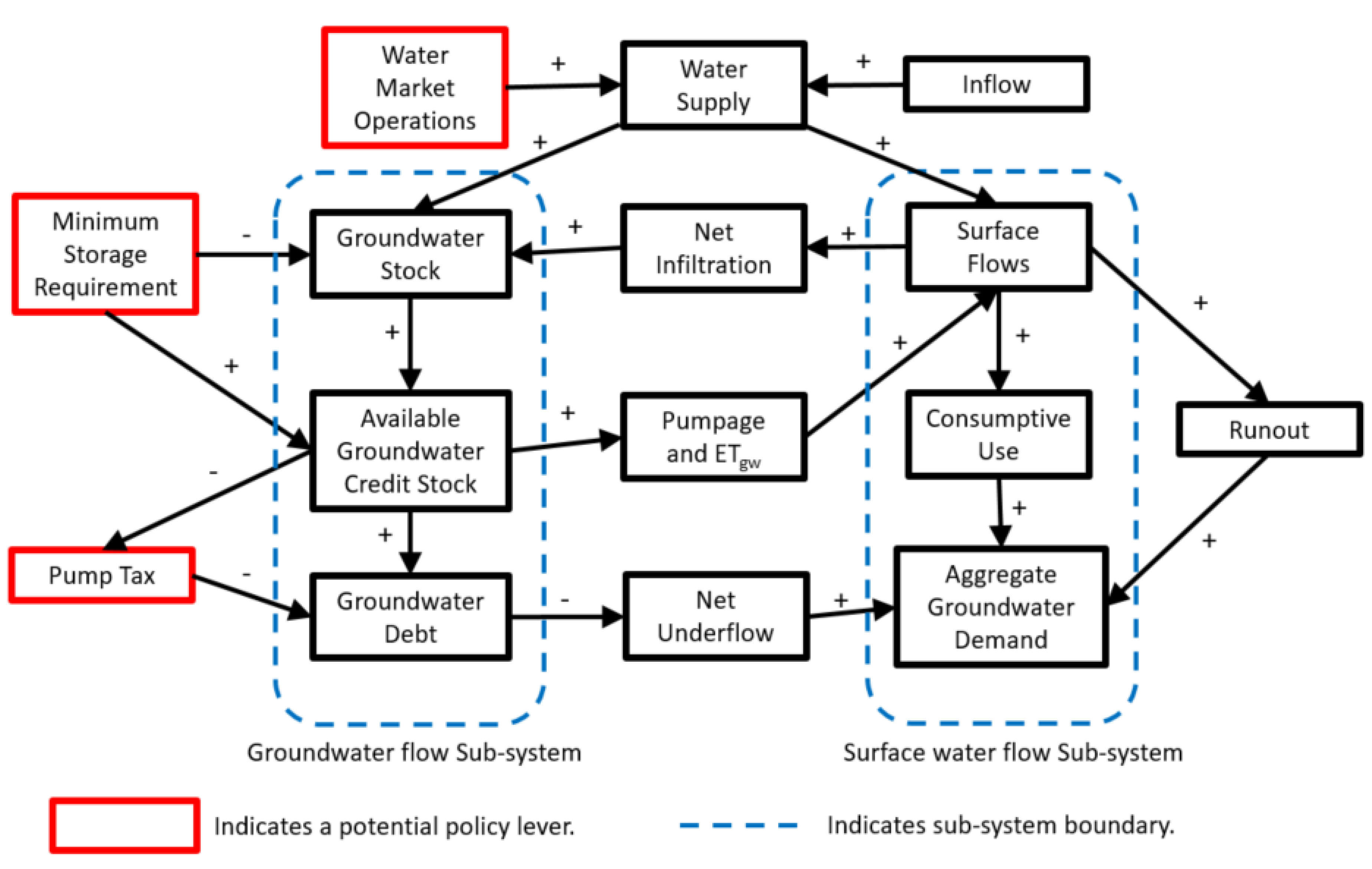
The general model shown in Figure 1 illustrates the system structure. It includes input components, policy levers, and the two sub-systems with transitional components in between. Input components are inflow, water supply, pumpage, and consumptive use. These can be supplied to the model based on historical data. In a planning effort, these components could be adjusted to simulate climate change, land use change, conservation efforts, or changes in consumption habits. The aggregate groundwater demand and groundwater debt components are artificial components intended to help explain the fate of groundwater over time. The available groundwater stock component is the total volume of groundwater available.

The policy levers shown represent potential policies that may be available to policy makers. These include water market operations, reserve requirements, and pump taxes. Water market operations include transferring water into or out of the system. Reserve requirements represent policies aimed at setting a physical limit to the amount of groundwater depletion. Pump taxes represent policies intended to increase the price of groundwater and potentially reduce demand.

The groundwater sub-system and the surface water sub-system are connected by various transitional components to create the single complex system shown in the causal loop diagram (CLD) below.

In system dynamics, CLDs are used to describe the relationship between structural components in a system [17]. Figure 1 is a CLD for the general model, illustrating the relationship between the system components described in Table 1 above. The arrows in Figure 1 show how components are connected. The “+” and “−” symbols are used in system dynamics to illustrate the direction of change in one component relative to the change in the connected components. The “+” symbol indicates changes between system components moving in the same direction. The “−” indicates changes between system components moving in the opposite direction. These components and connections make up the structure of the system. The structure of the general model was applied to the basin-specific models.

2.2.2. Basin-Specific Model Development

System dynamics models for the Cuyama and Modesto groundwater systems were developed based on the structure of the general model using Microsoft Excel. Each groundwater system is unique. The general model simply describes the location of the system components in the overall system and their relation to other components. For the model to be useful, the general model was adapted to the specific groundwater basin in question. In a basin-specific model, the components of the general model become parameters. Changes in these parameters cause changes in the other internal parameters based on the correlation equations used within the model. These, in turn, cause changes in estimated annual groundwater storage.

The parameters used for these models are the components of the groundwater system that make up the mass balance. Within the model, they are classified as input parameters and simulated parameters. The input parameters include water supply (i.e., rainfall and surface inflow), demand (i.e., evapotranspiration and consumptive use), and initial conditions for the groundwater system. Although it is beyond the scope of this research, the input parameters can be changed for planning purposes to simulate changes in climate, policy, or land use. The model simulates the remaining parameters during each water year run.

The general model provided the basic structure for each basin-specific model. However, the relationships between elements within each model were further refined by examination of data provided by USGS numerical models. In some cases, the components of the general model were sub-divided based on the available data. For example, in the Cuyama model, the net infiltration component was sub-divided into deep percolation and stream leakage parameters because the data for each parameter were available.

In order to develop the correlation equations required for the model to function, data provided by USGS numerical models were evaluated for evidence of strong correlations. For example, in the Cuyama basin, runoff was strongly found to be strongly correlated to precipitation, and stream leakage was correlated to runoff. This information was used to refine the linkages in the model and justify the development of the correlation equations used in the sub-basin model.

Once the correlated parameters were identified, regression analysis was used to develop the initial linear equations for the model using the earliest 10 years of data from USGS numerical models (see Tables 3 and 5 below). New correlation equations are developed after each time step (one simulated year). The slope and y-intercept values for each linear correlation equation are revised based on the new data developed within the simulation model. The model continues to develop linear equations based on the 10 years of data immediately preceding the simulation term. However, after each time step, the oldest data point from the USGS numerical model is replaced with new data developed within the system dynamics model, and new correlation equations are developed.

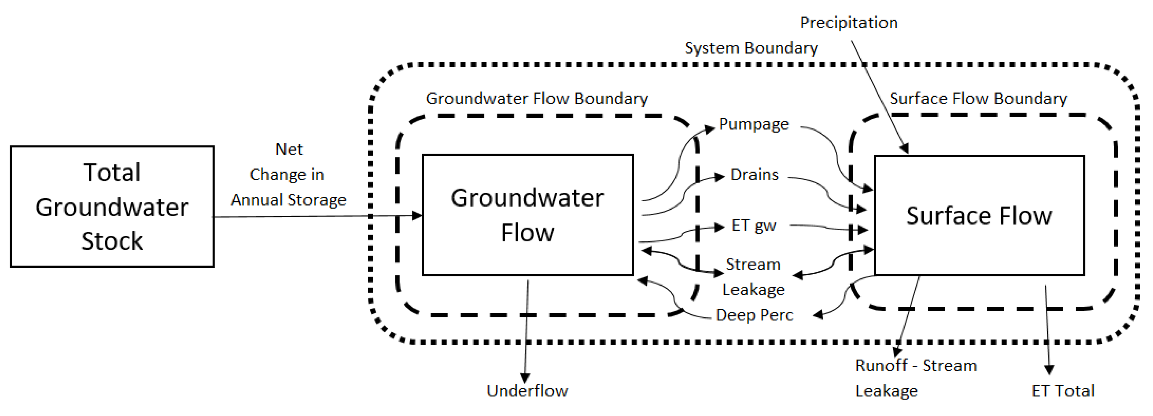
Values for the input parameters (initial conditions, supply, and demand) were entered into the models and used to calculate values for the simulated parameters via the linear equations. The model used these simulated internal parameters to generate new values for the linear correlation equations and calculate the net annual change in groundwater storage at each sub-system boundary (see Figure 2 and Figure 3). The annual change in groundwater storage calculated at the groundwater flow and surface water flow sub-system boundaries was then averaged to calculate the net annual change in groundwater storage for each year. This process was repeated for each year of the simulation. The following sections describe the structure and parameters of each basin-specific model.

2.2.3. Cuyama System Structure and Parameters

The Cuyama groundwater system is relatively simple. The water supply for consumptive use comes from precipitation or groundwater. Agriculture is by far the most significant demand component. Surface water runout and net underflow are generally small. Evapotranspiration represents the major outflow from the system. Figure 2 shows a graphical representation of the system.

The internal components of the Cuyama system indicate flow from one sub-system to the other sub-systems. Pumpage, drains, and groundwater evapotranspiration flow from the groundwater flow system to the surface flow system. The Excel model links the system parameters to each other based on observed relationships in the USGS data. For example, the annual volume of stream leakage was correlated to annual precipitation and deep percolation.

Table 2. Cuyama groundwater system input parameters and equations [17].

Parameter	Description	Equation
Precipitation (P)	Rainfall input parameter.	N/A—Input parameter
Total Evapotranspiration (ET all)	Evapotranspiration from surface and groundwater sources.	N/A—Input parameter
Evapotranspiration from Irrigation (ET irr)	Evapotranspiration from irrigated agriculture.	N/A—Input parameter
Aggregate Irrigation Efficiency (IE)	Percent of applied irrigation water contributing ET irr on an annual basis (%). Relates ET irr to groundwater demand.	IE = Pumpage from Ag Wells/ET irr
Pumpage (Pump)	Total annual pumpage from groundwater.	N/A—Input parameter

provides a description of each parameter used in the Cuyama groundwater model.

In numerical models, the value of system parameters is calculated using finite difference methods [11]. However, in the Cuyama system dynamics model, they are calculated using linear correlation equations. Long-term flow data are needed to develop the correlation equations. For model development, output from the CUVHM was used to identify correlated parameters. Based on this observed correlation, linear equations were developed to simulate parameters in the Cuyama system dynamics model.

Table 3. Cuyama simulated parameters and correlation equations [17].

Parameter	Correlated Parameter	Initial Correlation Equation
Runoff (R)	Precipitation	R = −0.29P − 15,026
Stream Leakage (SL)	Runoff	SL = −1.09R − 17,173
Deep Percolation (DP)	Precipitation	DP = 0.16P − 145.8
Drains (D)	Correlated to drains from the previous year (strong autocorrelation).	Dn = 0.9894Dn−1 + 1.0099
Evapotranspiration from groundwater (ET gw)	Correlated to ET gw from the previous year (strong autocorrelation).	Rout = R − SL

shows the internal system parameters used in the model to simulate the interaction between sub-systems.

2.2.4. Modesto System Structure and Parameters

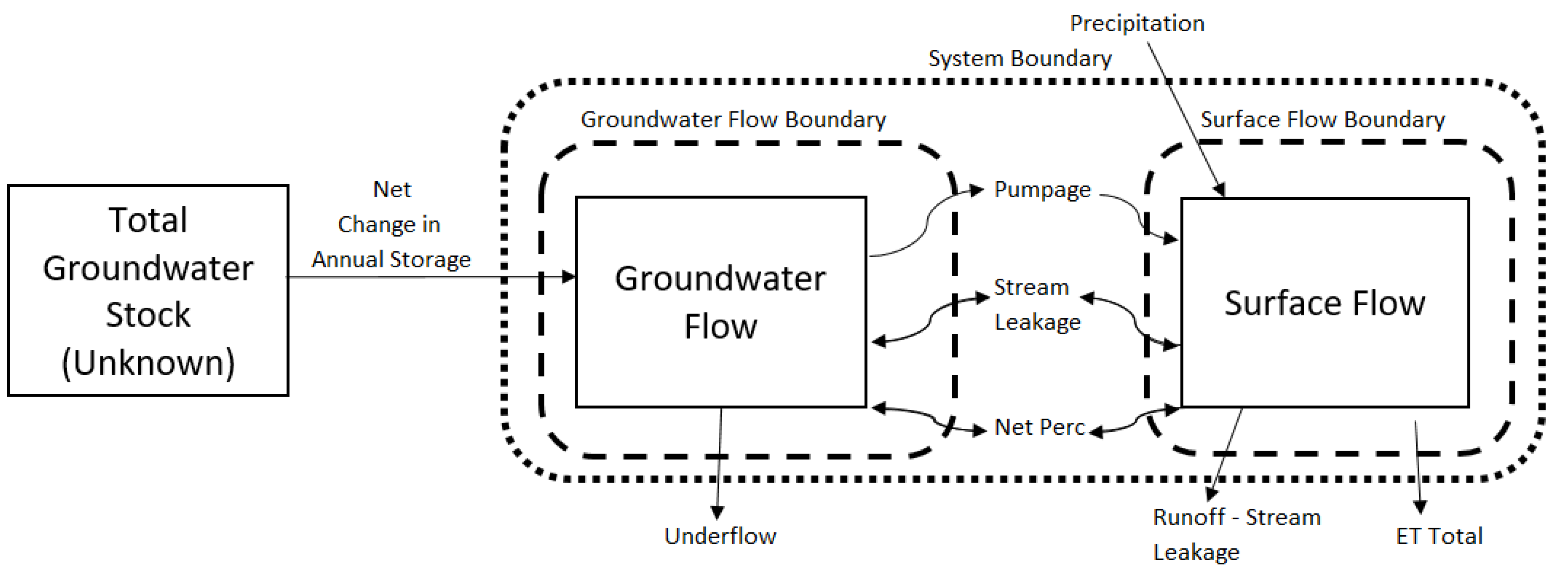
The Modesto groundwater system is larger than the Cuyama system. The water supply for consumptive use comes from precipitation, groundwater and surface water deliveries from outside the system boundary. Agriculture is the most significant demand component, while municipal use makes up the second most significant portion of overall consumption. Surface water runout and net underflow are large outflow components relative to consumption, while evapotranspiration represents the major outflow from the system. Figure 3 shows a graphical representation of the Modesto system.

The internal components of the Modesto system also indicate flow from one sub-system to the other sub-systems. The Excel model links the system parameters to each other based on observed correlations in the USGS MERSTAN model outputs. These relationships are simulated using linear correlation equations based on 10 years of data immediately preceding the simulation period.

Table 4. Modesto Basin input parameters [17].

Parameter	Correlated Parameter	Type
Precipitation (P)	Rainfall input parameter.	Input parameter
Total Evapotranspiration (ET all)	Evapotranspiration from surface and groundwater sources.	Input parameter
Surface Water Deliveries (SWD)	Surface water deliveries for irrigation	Input parameter
Farm Well Pumpage (Wf)	Annual volume of pumpage for irrigation.	Input parameter
Domestic Wells (Wd)	Annual volume of pumpage for rural domestic use.	Input parameter
Municipal Pumpage (M)	Annual volume of pumpage for municipal use.	Input parameter

provides a description of each input parameter used in the Modesto groundwater model.

Table 5. Modesto simulated parameters and correlation equations [17].

Parameter	Correlated Parameter	Initial Correlation Equation
Aggregate Irrigation Efficiency (IE)	Percent of applied irrigation water contributing ET irr on an annual basis (%). Relates ET irr to Wf.	IE = Wf/ET irr.
Stream Leakage (SL)	Underflow (UF)	SL = −0.937UF − 97,325
Net annual groundwater Underflow (UF)	Farm Wells (Wf)	UF = −0.193Wf − 28,617
Parameter	Correlated Parameter	Equation
Reservoir Leakage (RL)	Net Percolation (Net Perc))	RL = −0.005NetPerc − 28,833
Net Percolation to groundwater (Net Perc)	Runoff to streams (R)	NetPerc = −192.33R − 35,264.7

shows the internal system parameters used to simulate the interaction between sub-systems and the correlation equations derived from the USGS MERSTAN model output.

2.3. Model Equations

The basin-specific models use supply and demand inputs to predict changes in groundwater storage for 1-year, 5-year, and 10-year periods based on the previous 10-year period. Input parameters were taken directly from USGS data. Linear correlation equations were used to predict the value of internal parameters. These linear equations are based on relationships developed from the USGS numerical models over the 10 years immediately preceding the period being simulated. As the model advances, values of the internal parameters derived from simulation are replaced by simulated values and the coefficients of the linear equations are updated to reflect the state of the new system.

The models calculate the change in groundwater storage on an annual basis by mass balance. The mass balance is computed at the overall system boundary and the groundwater flow system boundary (see Figure 2) and then averaged to estimate the annual change in groundwater storage. Each model uses slightly different equations to estimate the change in storage due to the different parameters used for simulation. The annual change in groundwater storage for the Cuyama system is calculated at the system boundary using the following equation [19]:

$$\Delta {\mathrm{S}}_{\mathrm{bdry}}=\mathrm{P}-{\mathrm{ET}}_{\mathrm{all}}-{\mathrm{R}}_{\mathrm{out}}$$

(1)

where DS_bdry = net annual change in storage calculated at the system boundary, P = annual precipitation, ET_all = annual evapotranspiration, R_out = annual runout.

The net annual change in groundwater storage is calculated at the groundwater flow boundary using the following equation:

$$\Delta {\mathrm{S}}_{\mathrm{GW}}=\left(\mathrm{DP}+\mathrm{SL}\right)-\left({\mathrm{ET}}_{\mathrm{gw}}+\mathrm{D}+\mathrm{Pump}+\mathrm{UF}\right)$$

(2)

where DS_GW = net annual change in storage calculated at the groundwater system boundary, DP = annual deep percolation, SL = net annual stream leakage, ET_gw = annual evapotranspiration from groundwater sources, D = net annual flow from drains, Pump = annual groundwater pumpage, UF = net annual groundwater underflow.

The model calculates the annual change in storage by taking the average of the values calculated at each boundary using the following Equation [19]:

$$\Delta {\mathrm{S}}_{\mathrm{Calc}}=\frac{\Delta {\mathrm{S}}_{\mathrm{GW}}+\Delta \mathrm{brdy}}{2}$$

(3)

where DS_Calc = simulated net annual change in storage, DS_GW = net annual change in storage calculated at the groundwater system boundary, DS_bdry = net annual change in storage calculated at the system boundary.

The USGS model for the Modesto system calculates the change in groundwater storage differently than the Cuyama system due to the nature of the data available from the USGS MERSTAN Model. Due to the way time series output is identified in the USGS MERSTAN model, the net annual change in groundwater storage for year t is calculated using output from the previous year (t − 1). The net annual change in groundwater storage at the system boundary (see Figure 3) is calculated using the following equation [19]:

$$\Delta {\mathrm{S}}_{\mathrm{bdry}}=\left(\mathrm{P}-{\mathrm{ET}}_{\mathrm{all}}-{\mathrm{R}}_{\mathrm{out}}-\mathrm{UF}-\mathrm{RL}-\mathrm{SL}\right)$$

(4)

where DS_bdry = net annual change in storage calculated at the system boundary for year t, P = annual precipitation for year t − 1, ET_all = annual evapotranspiration for year t − 1, R_out = annual runout for year t − 1, UF = net annual groundwater underflow for year t − 1, RL = net annual reservoir leakage for year t − 1, SL = net annual stream leakage for year t − 1.

The annual change in groundwater storage for year t is calculated at the groundwater flow boundary using the following equation [19]:

$$\Delta {\mathrm{S}}_{\mathrm{GW}}=\left(\mathrm{Perc}+\mathrm{SL}\right)-\left({\mathrm{W}}_{\mathrm{F}}+{\mathrm{W}}_{\mathrm{d}}+\mathrm{UF}\right)$$

(5)

where DS_GW = net annual change in storage calculated at the groundwater system boundary for year t, Perc = net annual deep percolation year t − 1, SL = net annual stream leakage for year t − 1, W_F = annual farm pumpage for year t − 1, W_d = annual domestic pumpage for year t − 1, UF = net annual groundwater underflow for year t − 1.

The model calculates the annual change in storage by taking the average of the values calculated at each boundary in the same way as the Cuyama model using Equation (3) above.

The basin-specific system dynamics models predict changes in groundwater storage for 1-year, 5-year, and 10-year periods based on input from the previous 10-year period. The coefficients used to calculate internal values update with each successive simulation to reflect changes in the new 10-year period. This process was repeated for all available 5-year and 10-year periods for which data from the preceding 10 years were available.

Output from the CUVHM provides annual estimates for net groundwater storage for the Cuyama groundwater basin from 1950 to 2010. The same information is provided for the Modesto region from 1960 to 2004. Output from the basin-specific system dynamics models were compared to output form the USGS MERSTAN and CUVHM models for verification.

2.4. Statistical Analysis

Traditional statistical tests are often not applicable for system dynamics modeling [14]. These tests typically rely on assumptions of normality, stationarity, and equal variance [13] that do not apply to system dynamics because system dynamics models rely on correlation and covariance between parameters to function. As such, the assumptions pertaining to traditional statistical techniques are violated. Sterman [14] suggests using Theil inequality statistics and root mean square percent error (RMSPE) to evaluate system dynamics models. RMSPE is used to assess goodness of fit. Theil inequality statistics provide a method for error decomposition. Regression analysis, although not technically appropriate for system dynamics, is used provide a basis for comparison with traditional statistical methods.

2.4.1. Root Mean Square Percent Error

Mean square error is a common measure of error in forecast models. RMSPE is a similar statistical technique that is considered appropriate for evaluating system dynamics models [14]. RMSPE expresses error as a percentage of the expected value. The equation for RMSPE is presented below:

$$\sqrt{\frac{1}{\mathrm{n}}{\displaystyle \sum }_{\mathrm{t}=1}^{\mathrm{n}}{\left[\frac{\left(\mathrm{St}-\mathrm{At}\right)}{\mathrm{At}}\right]}^2}$$

(6)

where n = number of observations, St = simulated value at time t, At = actual value at time t.

An RMSPE value of less than 5% is considered acceptable for this research. This is based on a review of the literature on system dynamics models and accounts for the fact that the purpose of these models is only to predict with a level of accuracy necessary for planning and to aid in conceptual understanding. Qudrat-Ullah and Seong (2010) [20] suggested an RMSPE range from 3% to 4%, whereas Tidwill et al. (2004) [21] used a value of 7%.

2.4.2. Theil Inequality Statistics

Theil inequality statistics are considered to be an appropriate summary statistic for use with system dynamics models [16] because they can be used to quantify sources of error between simulated and observed behavior. They can be used to separate the fractions of total error associated with bias, unequal variance, and unequal covariance, according to Equations (7) to (10) [14].

U^M + U^S + U^C = 1

(7)

where U^M = fraction of total MSE from bias, U^S = fraction of total MSE from unequal variance, U^C = fraction of total MSE from unequal covariance.

The equations used to calculate Theil statistics are

$${\mathrm{U}}^{\mathrm{M}}=\frac{{\left(\overline{S}-\overline{A}\right)}^2}{\frac{1}{n}\sum {\left(St-At\right)}^2}$$

(8)

where n = number of observations, St = simulated value at time t, At = Actual value at time t, $\overline{S}$ = mean of simulated values, $\overline{A}$ = mean of actual values;

$${\mathrm{U}}^{\mathrm{S}}=\frac{{\left(S_S- S_A\right)}^2}{\frac{1}{n}\sum {\left(St-At\right)}^2}$$

(9)

where n = number of observations, St = simulated value at time t, At = actual value at time t, S_S = standard deviation of simulated values, S_A = standard deviation of actual values;

$${\mathrm{U}}^{\mathrm{c}}=\frac{2 \left(1-r\right)S_S{S}_A}{\frac{1}{n}\sum {\left(St-At\right)}^2}$$

(10)

where n = number of observations, St = simulated value at time t, At = actual value at time t, S_S = standard deviation of simulated values, S_A = standard deviation of actual values, r = coefficient of correlation.

Because system dynamics models build causal relationships into the model, the fraction of total error due to unequal variance and covariance (U^S and U^C) is expected to be large [16]. Conversely, an adequate system dynamics model should display minimal systemic bias (i.e., low U^M). Based on a review of system dynamics modeling literature, U^M should be less than 10% of the total error.

2.4.3. Coefficient of Determination (R²)

Regression analysis is generally considered inappropriate for evaluating system dynamics models [16] due to the expected unequal variance associated with these models. In this research, the coefficient of determination was provided as a basis for comparison with traditional statistical methods in order to illustrate the goodness of fit. A coefficient of determination (R²) of 0.90 or greater was considered adequate for the purposes of this model based on a review of the literature on other system dynamics models.

3. Results

Models were developed for each groundwater basin using 1-year, 5-year, and 10-year simulation periods. Each model was tested for goodness of fit (RMSPE), cumulative error, systemic bias (U^M), and the coefficient of determination (R²).

3.1. Basin 1-Year Simulation Period Results

The Cuyama groundwater model simulates the change in groundwater storage from water year 1960 to 2010. The Modesto groundwater model simulates the change in groundwater storage from water year 1970 to 2003.

Table 6. Comparison of results for the 1-year simulation.

Basin	USGS Numerical Model (Million m3)	System Dynamics Model (Million m3)	Difference (Million m3)	% Error	RMSPE	R2	UM
Modesto	−4441	−4236	−205	4.60%	0.1	0.88	0.30%
Cuyama	−2168	−2150	−18	0.80%	45.1	0.90	0.90%

shows the predicted changes in storage for each model and summarizes the results of the 1-year simulations.

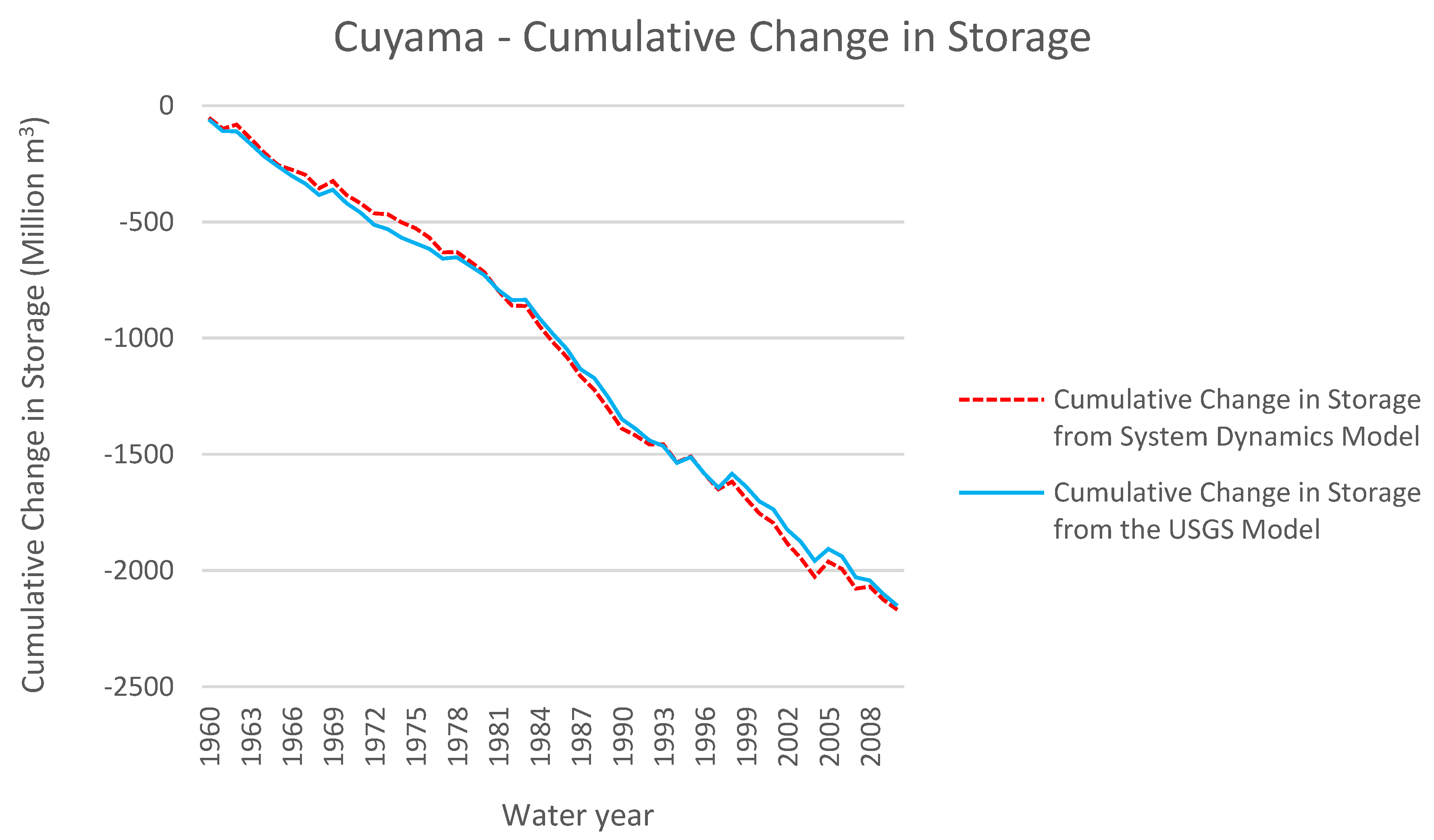
The 1-year simulations use 10 years of data to predict the annual change in storage for the next year. As Table 6 illustrates, these models predict change in storage well, with the exception of the RMSPE in the Cuyama model. However, this error is due to a single large error in 1993. In water year 1993, the actual change in storage was 76,500 m³. The simulated change in storage was approximately −24,000,000 million m³. This error is likely due to the unusually high rainfall that occurred in 1993 and land use changes during the same period [15]. Large rainfall in 1993 is linked to a strong El Nino event. If water year 1993 is removed from the calculation, the RMSPE for the remaining years is excellent (0.74). Figure 4 below shows that the cumulative change in storage calculated by the Cuyama system dynamics model closely matched the output from the CUVHM model developed by the USGS when using 1-year simulation.

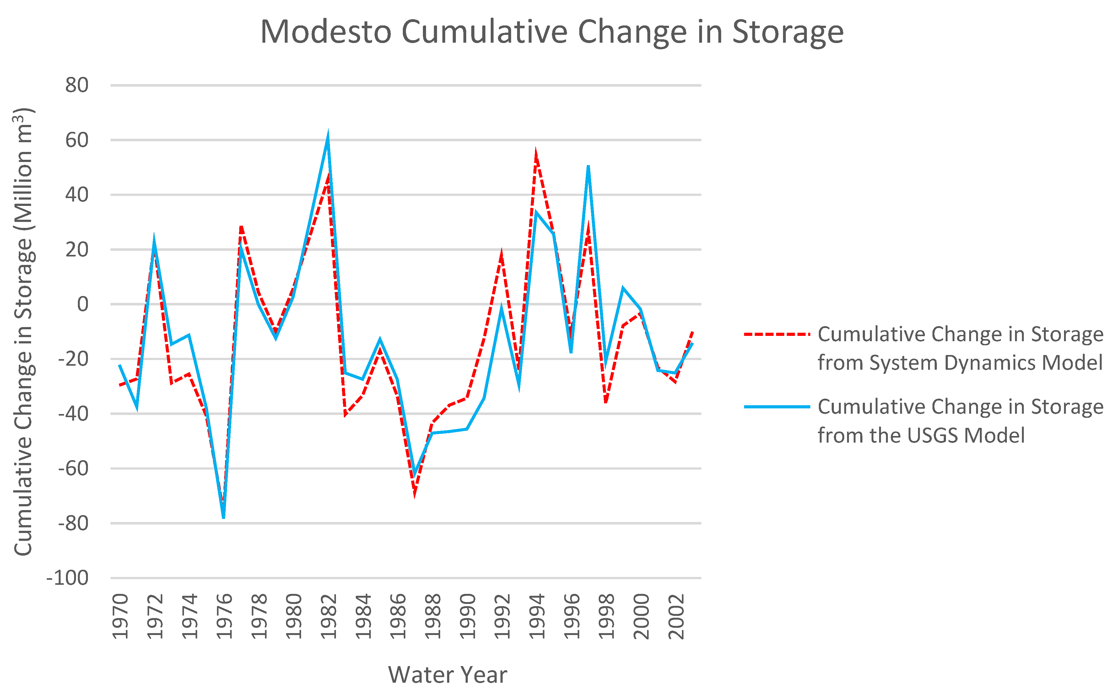
The Modesto model also performs well in 1-year simulations. The cumulative error after 34 1-year simulations was only 4.6%. Systemic bias and RMSPE were low. The R² value of 0.88 was slightly lower than desirable but may be acceptable for the purposes of testing groundwater policy. Figure 5 below shows that the cumulative change in storage calculated by the Modesto system dynamics model closely matched the output from the USGS MERSTAN model when using 1-year simulation.

3.2. Basin 5-Year Simulation Period

The 5-year simulations use 10 years of data to simulate the next five years. All available 5-year periods were simulated and the results were averaged in order to evaluate the model over the entire time span available from the USGS data.

Table 7. Results of the 5-year simulations.

Basin	Term	Average Error/Term (%)	Median Error/Term (%)	Average UM	Average R2	Average RMSPE
Modesto	5-year	244%	2.1%	44.6%	0.92	0.59
Cuyama	5-year	−0.90%	0.1%	42.9%	0.93	17.59

shows the averages of the results for the 5-year simulations.

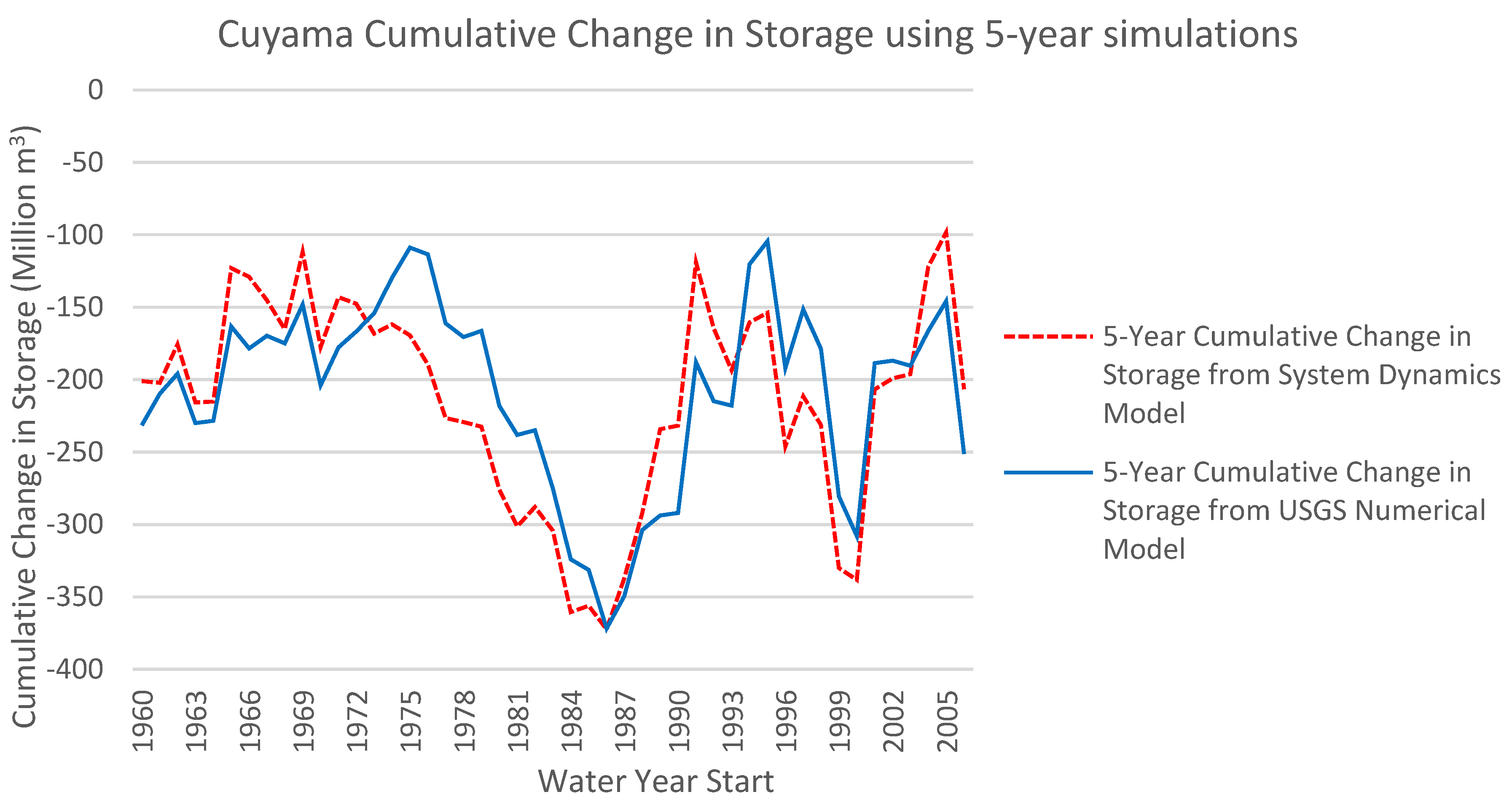
The Cuyama model predicts change in storage well for the 5-year simulation periods. The RMSPE is high due to the results of simulations that include 1993. As discussed above, the unusually high rainfall in 1993 was an anomaly in the data. The Cuyama model also shows significant systemic bias due to the inability of the model to react to abrupt changes in rainfall that are not present in the 10-year period preceding the simulation. However, R² and average error appear adequate for planning purposes. The median error is also low. As Figure 6 shows, the system dynamics model matched the USGS model results closely. Although the results for any 5-year simulation vary, the system dynamics model captures the changes and overall trends.

The Modesto model shows a large average percent error in the 5-year simulations. This is also due to large rainfall events, as evident by the relatively low median error. The 5-year simulations show high R² values and low median and root mean square errors. As Figure 7 shows, the system dynamics model captures the overall trends fairly well.

3.3. 10-Year Simulation Period

The 10-year simulations used 10 years of data to simulate the change in groundwater storage over the next 10 years. All available 5-year and 10-year periods were simulated, and the results were averaged in order to evaluate the model over the entire time span available from the USGS data.

Table 8. Results of the 10-year simulations.

Basin	Term	Average Error/Term (%)	Median Error/Term (%)	Average UM	Average R2	Average RMSPE
Modesto	10-year	635%	21.8%	19.7%	0.83	0.8
Cuyama	10-year	3.30%	2.3%	33.4%	0.91	24.82

shows the averages of the results.

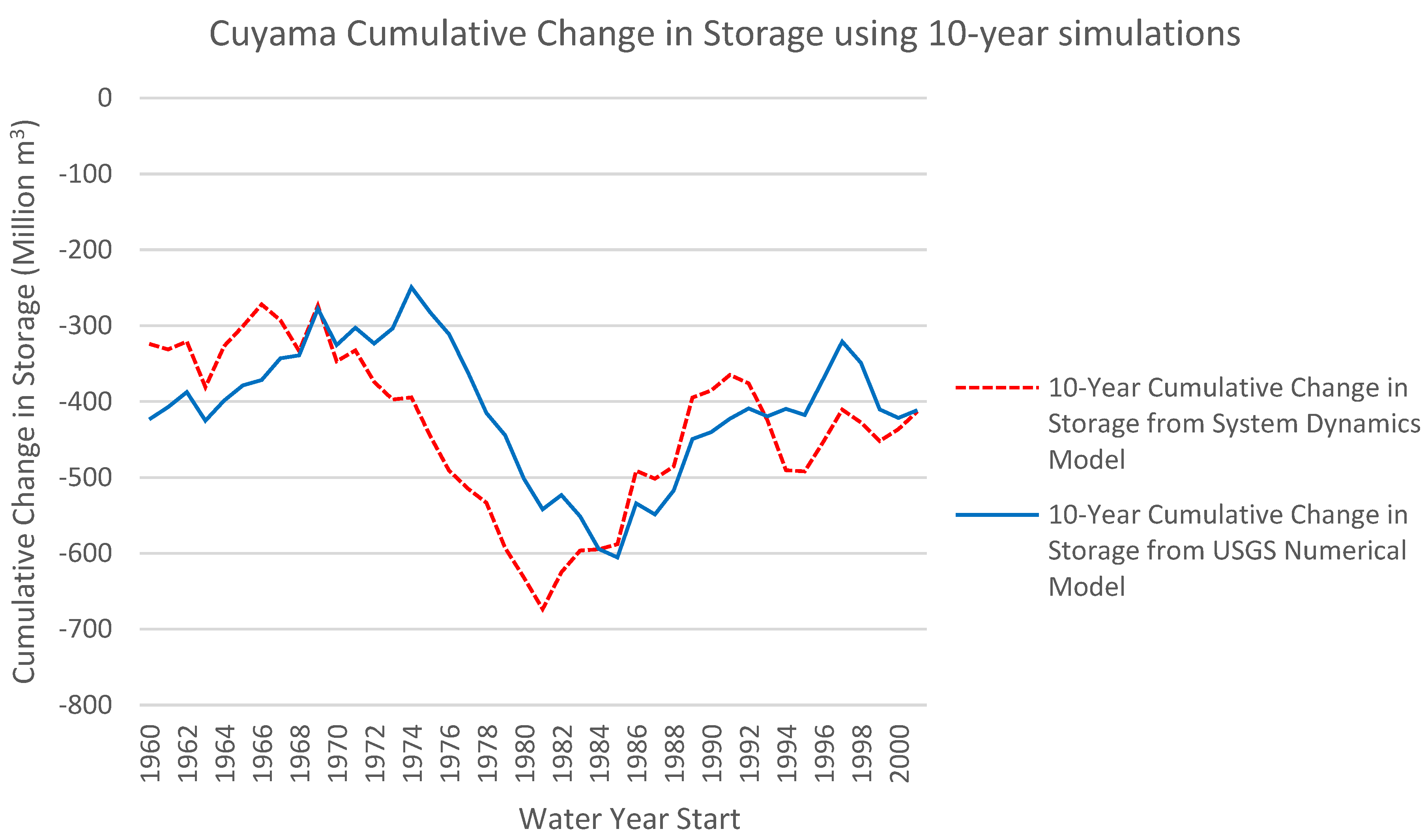
The Cuyama model predicts change in storage well for the 10-year simulation periods. R² and average error appear adequate for planning purposes, and the median error is low. However, the RMSPE and U^M were high. Systemic bias is evident in Figure 8 below.

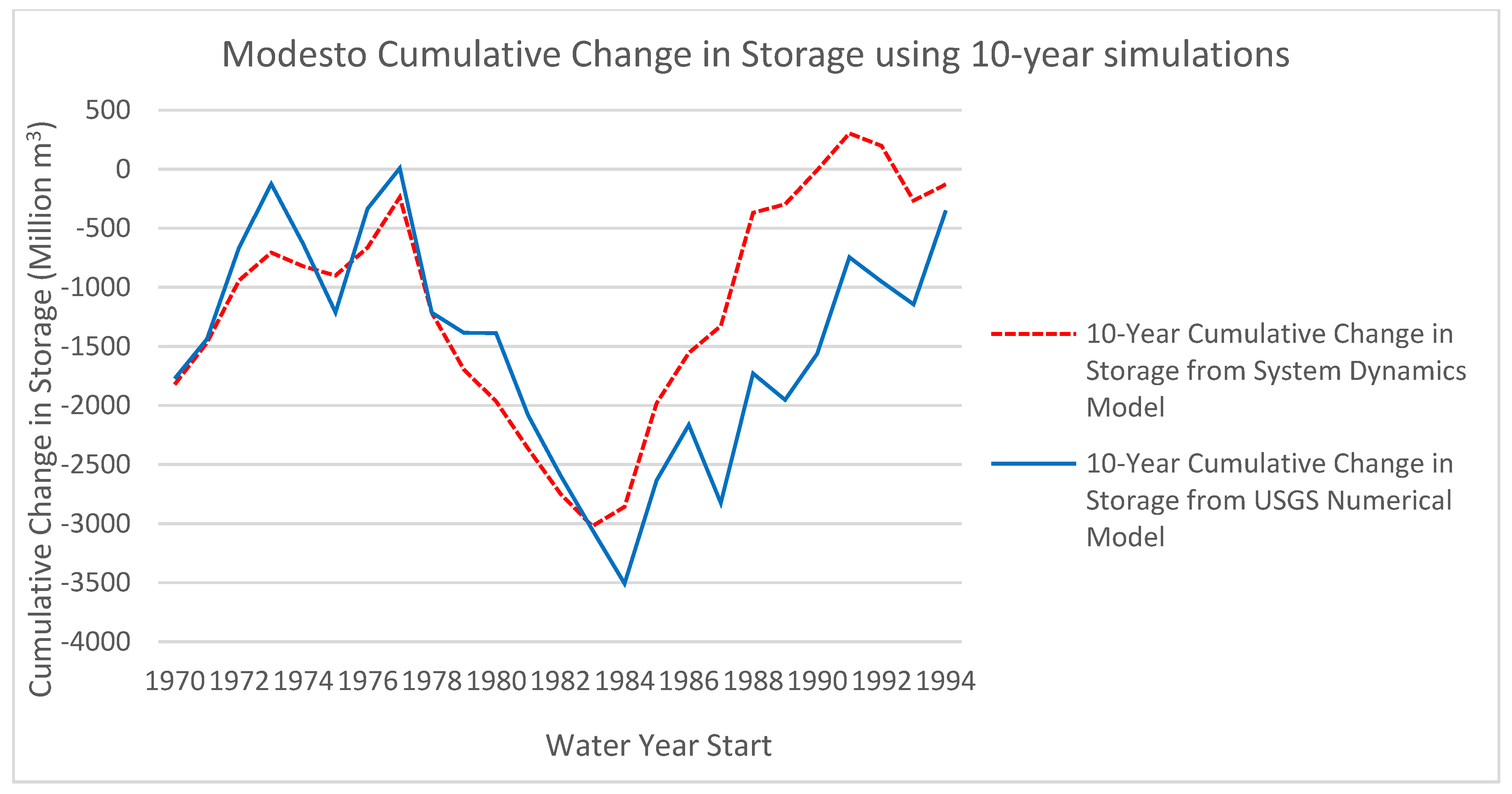
The Modesto model shows a large average percent error and median error in the 10-year simulations. R² was lower than desirable, indicating that this simulation is probably not acceptable for planning purposes. Figure 9 below shows that the system dynamics model did not match the USGS MERSTAN model well from the 10-year simulations.

4. Discussion

The models presented above use correlation equations to simulate changing in stocks and flows rather than numerical methods to simulate physical processes. This is a simplification of very complex processes into simple input-output calculations based on observed correlations. However, for some planning efforts, the details of these physical processes may not be available or necessary. The models are limited in that they only estimate changes in net annual groundwater storage. They are not intended to fully characterize the properties or complex processes in a groundwater system. Another limitation is that flow data are required to develop the correlation equations that drive the model.

The results above indicate that the system dynamics models compare favorably to the numerical models developed by the USGS when using them for 1-year and 5-year simulation periods. The high R² values and low median errors indicate that the models are acceptable for planning purposes. However, the results also indicate that the 10-year simulation models may not be acceptable for planning purposes. Using 10 years of data to simulate 10 years into the future may not be appropriate for these system dynamics models.

The results also show that abnormally wet years can have a dramatic effect on the results. Future research should examine the difference in system response in wet years and dry years. These models can be improved by developing separate equations for wet and dry years due to the relationship between precipitation, runoff, and infiltration. Future research should also evaluate the impact of using nonlinear equations on predictive accuracy and ease of use. The models developed in this research use simple linear correlation equations to predict the behavior of internal system parameters in order to make the models simple, easy to understand, and relatively easy to develop. It is possible that the accuracy of the models developed in this research may be improved using nonlinear correlation equations.

5. Conclusions

Simulation models may help planners better understand groundwater systems and make better decisions about how to transition from over-exploitation of groundwater to sustainable groundwater management. The research presented indicates that it is possible to simulate complex groundwater system behavior using a system dynamics approach using observed correlations and linear equations. The simulation models discussed in this research require less hydrogeology expertise and are less data-intensive than other simulation models.

The models were subjected to statistical analysis relevant to system dynamics modeling. This analysis indicates that the models are likely sufficient for the purpose of testing groundwater policy with a simulation period of five years or less. The models can replicate changes in groundwater storage volumes provided by the USGS for 1-year and 5-year periods at a level suitable for testing groundwater policy. Although the Cuyama model was capable of replicating changes in groundwater storage for a 10-year simulation period, the Modesto model was not. These mixed results cause the authors to question whether the models are suitable for testing groundwater policy beyond five years. With further development, the system dynamics approach shown here may become a powerful decision support tool in the analysis and modeling of water management systems allowing for a more systemic view of these complex systems.

References

- Water in the West. Water and Energy Nexus: A Literature Review; Woods Institute for the Environment, Stanford University: Palo Alto, CA, USA, 2013. [Google Scholar]
- Carle, D. Introduction to Water in California; University of California Press: Berkeley, CA, USA, 2009. [Google Scholar]
- Green, T.; Taniguchi, M.; Kooi, H.; Gurdak, J.; Allen, D.; Hiscock, K. Beneath the surface of global change: Impacts of climate change on groundwater. J. Hydrol. 2011, 405, 532–560. [Google Scholar] [CrossRef] [Green Version]
- Sophocleous, M. From safe yield to sustainable development of water resources—The Kansas experience. J. Hydrol. 2000, 16, 27–43. [Google Scholar] [CrossRef]
- Xu, Z.X.; Takeuchi, K.; Ishidaira, H.; Zhang, X.W. Sustainability analysis for yellow river water resources using the system dynamics approach. Water Resour. Manag. 2002, 16, 239–261. [Google Scholar] [CrossRef]
- Bear, J.; Beljin, M.; Ross, R. Fundamentals of Ground-Water Modeling; United Stated Environmental Protection Agency: Superfund Technology Support Center for Ground Water, Robert S. Kerr Environmental Research Laboratory: Washington, DC, USA, 1992. [Google Scholar]
- United States Geological Survey. Comparison of Selected Methods for Estimating Groundwater Recharge in Humid Regions. In USGS Groundwater Information. Available online: https://water.usgs.gov/ogw/gwrp/methods/compare/method_details.php?method=ground_water (accessed on 20 April 2019).
- Theis, C.V. The source of groundwater from Wells. Civ. Eng. 1940, 10, 277–280. [Google Scholar]
- California Association of Water Agencies. Sustainable Groundwater Management Act of 2014 Fact Sheet. 2014. Available online: www.acwa.com (accessed on 7 July 2019).
- Langridge, R.; Daniels, B. Accounting for climate change and drought in implementing sustainable groundwater management. Water Resour. Manag. 2017, 31, 3287–3298. [Google Scholar] [CrossRef]
- California Department of Water Resources. Draft Hydrogeologic Conceptual Model Best Managment Practices; California Department of Water Resources: Sacramento, CA, USA, 2016. [Google Scholar]
- Winz, I.; Brierley, G.; Trowsdale, S. The use of system dynamics simulation in water resource management. Water Resour. Manag. 2009, 23, 1301–1323. [Google Scholar] [CrossRef]
- Barlas, Y. Multiple tests for validation of system dynamics type simulation models. Eur. J. Oper. Res. 1989, 42, 59–87. [Google Scholar] [CrossRef]
- Sterman, J. Appropriate summary statistics for validating the historical fit of system dynamics models. Dynamica 1984, 10, 51–66. [Google Scholar]
- Hanson, R.T.; Flint, L.; Faunt, C.C.; Gibbs, D.R.; Schmid, W. Scientific Investigations Report 2014-5150 Version 1.1: Hydrologic Models and Analysis of Water Availability in Cuyama Valley, California; U.S. Geological Survey: Reston, VA, USA, 2015.
- Philips, S.; Rewis, D.L.; Traum, J.A. Scientific Investigations Report 2015-5045: Hydrologic Model of the Modesto Region, California, 1960–2004; U.S. Geological Survey: Reston, VA, USA, 2015.
- Bates, G.; Beruvides, M. Financial and groundwater credit in contractionary environments: Implications for sustainable groundwater management and the groundwater credit crunch. In Proceedings of the 2015 International Annual Conference of the American Society for Engineering Management, Indianapolis, IN, USA, 7–10 October 2015. [Google Scholar]
- Bates, G.; Beruvides, M. Systemic similarities between groundwater management and monetary policy: Implecations for sustainable groundwater management. In Proceedings of the 2017 International Annual Conference of the American Society for Engineering Management, Huntsville, AL, USA, 18–21 October 2017. [Google Scholar]
- Bates, G. A Systems Analysis of Sustainable Groundwater Management in California: Homology and Isomorphology with Monetary Policy. Ph.D. Thesis, Texas Tech University, Lubbock, TX, USA, 2017. [Google Scholar]
- Qudrat-Ullah, H.; Seong, B.S. How to do structural validity of a system dynamics model type simulation model: The case of an energy policy mode. Energy Policy 2010, 38, 2216–2224. [Google Scholar] [CrossRef]
- Tidwell, V.C.; Passell, H.D.; Conrad, S.H.; Thomas, R.P. System dynamics modeling for community-based water planning: Application to the middle Rio Grande. Aquat. Sci. 2004, 64, 357–372. [Google Scholar] [CrossRef]
Figure 2.
Cuyama groundwater system.
Figure 3.
Modesto groundwater system.
Figure 4.
Comparison of cumulative change in storage for the Cuyama models.
Figure 5.
Comparison of cumulative change in storage for the Modesto models.
Figure 6.
Cuyama Basin 5-year groundwater system simulation.
Figure 7.
Modesto Basin 5-year groundwater system simulation.
Figure 8.
Cuyama Basin 10-year groundwater system simulation.
Figure 9.
Modesto Basin 10-year groundwater system simulation.