Dependence Between Extreme Rainfall Events and the Seasonality and Bivariate Properties of Floods. A Continuous Distributed Physically-Based Approach

Abstract

This paper focuses on proposing the minimum number of storms necessary to derive the extreme flood hydrographs accurately through event-based modelling. To do so, we analyzed the results obtained by coupling a continuous stochastic weather generator (the Advanced WEather GENerator) with a continuous distributed physically-based hydrological model (the TIN-based real-time integrated basin simulator), and by simulating 5000 years of hourly flow at the basin outlet. We modelled the outflows in a basin named Peacheater Creek located in Oklahoma, USA. Afterwards, we separated the independent rainfall events within the 5000 years of hourly weather forcing, and obtained the flood event associated to each storm from the continuous hourly flow. We ranked all the rainfall events within each year according to three criteria: Total depth, maximum intensity, and total duration. Finally, we compared the flood events obtained from the continuous simulation to those considering the N highest storm events per year according to the three criteria and by focusing on four different aspects: Magnitude and recurrence of the maximum annual peak-flow and volume, seasonality of floods, dependence among maximum peak-flows and volumes, and bivariate return periods. The main results are: (a) Considering the five largest total depth storms per year generates the maximum annual peak-flow and volume, with a probability of 94% and 99%, respectively and, for return periods higher than 50 years, the probability increases to 99% in both cases; (b) considering the five largest total depth storms per year the seasonality of flood is reproduced with an error of less than 4% and (c) bivariate properties between the peak-flow and volume are preserved, with an error on the estimation of the copula fitted of less than 2%.

1. Introduction

Distributed physically-based hydrological models (DHMs) appeared in the 1960s and have been the object of critics due to their complexity and difficulty of use [1]. Nowadays, the availability of higher resolution spatio-temporal datasets, the appearance of high performance computers, and the development of parallel-computing [2,3,4,5] have opened the possibility of using these models for large size basins and long-term hydrological continuous simulations. Thus, challenges such as the influence of land-use changes [6,7] or the impact of climate change [8,9] on the involved hydrological processes can be analyzed with these approaches.

Another use of distributed hydrological models is the estimation of extreme floods for the design of civil infrastructures, such as bridges, levees, or dams. For these structures, it is necessary to estimate hydrographs of low probability of occurrence, that is, with return periods that go from hundreds to thousands of years in the case of dams [10]. Several methods can be applied and are mainly classified according to two main groups: Statistical flood frequency analysis, and derived flood frequency (DFF) simulation methods. Statistical methods need large flow records (hardly available [11,12]), have the drawback of the uncertainty associated to the distribution fitting for large return periods [13], and provide a value of peak-flow, volume, or duration but not the hydrograph shape. Furthermore, when they are applied in ungauged basins, the physical processes that occur in the watershed are not usually considered and the uncertainty on the flood quantiles estimation increases [14].

Due to these reasons, DFF methods are generally preferred over statistical ones [15]. DFF can be divided into two approaches: Continuous simulation and stochastic event-based methods [15]. Using a DHM, we are able to derive flood frequency distributions from the continuous hourly streamflow obtained at any desired point in the drainage network of the basin by forcing the DHM with an hourly stochastic weather generator. This approach has the advantage of estimating the variables for the entire period of simulation. However, continuous models tend to be more complex than stochastic event-based models, with computational efforts that could be very intensive, even when using high performance computing and parallelization processes. On the other hand, event-based simulations require much shorter simulation times. However, these methods are based on the assumption that the flood hydrograph has the same return period as the storm event, which is not realistic [16,17,18]. Furthermore, different properties of storm events could affect the derivation of flood frequency curves: Rainfall temporal distribution, event duration, maximum intensity, and total storm depth, among others.

Examples of both DFF approaches can be found in the existing literature. In the case of event-based approaches, some studies have combined non-complex stochastic storm generators (i.e., [19,20]) or complex rainfall generators (i.e., [21]); with semidistributed (i.e., [22]) or distributed models (i.e., [23]). In the case of continuous simulations, in order to reduce the computational cost, most authors have worked with lumped or semidistributed models (i.e., [24,25]), and some of them have worked with distributed models by using high performance computers [2,3,4,5].

To overcome the limitations in the two approaches, several authors have proposed combining event-based models with continuous models. Paquet et al. [26] proposed the SCHADEX model, which consists of replacing stochastic rainfall events within a short continuous simulation with observed data and a Monte Carlo framework. Li et al. [15] developed the hybrid-CE approach, which consists of combining a continuous long-term simulation of rainfall and short continuous simulations to probabilistically characterize the rainfall and initial soil moisture (respectively) to force an event-based model. Both approaches [15,26] used lumped models.

The focus of this paper is, by using a fully physically-based DHM coupled with a stochastic weather generator in a continuous simulation, to provide a guideline to select the minimum necessary storm events that should be simulated in event-based approaches to obtain similar results to those obtained by continuous simulations in the derivation of flood frequency curves. Sordo-Ward et al. [27] carried out a similar analysis in some watersheds in mainland Spain, by using a semi-distributed event-based model coupled with a continuous stochastic rainfall generator. They separated all the events within the generated series and analyzed the relationship between the storms and the maximum annual peak-flow in the Manzanares river basin (Spain) and two of its sub-basins. Flores-Montoya et al. [23] also carried a similar analysis using a distributed event-based model in two basins in France. However, in both studies, the lack of a continuous simulation required the estimation of the initial soil moisture (same curve number value in [27] and probabilistically in [23]). Within this paper, the continuous simulation with a fully physically-based DHM enables to account for the variations of the initial soil moisture. Thus, not only can the magnitude and recurrence of events be analyzed, but also the relation between storms and the seasonality of the flood hydrographs. Furthermore, within this study, the relationship within storms and flood hydrographs is analyzed, not only in a univariate way, but with a bivariate approach through the use of copulas for a better assessment between the relation of storms and the dependence of the maximum annual peak-flow and volume.

Therefore, the objective is to propose a criterion for the selection of the minimum number of storm events per year to guarantee a correct derivation of the bivariate flood frequency curve, according to the following characteristics:

• Magnitude and recurrence of the maximum annual peak-flow and volume (univariate approach).
• Seasonality of the maximum annual peak-flow and volume (univariate approach).
• Dependence, magnitude, and recurrence of simultaneous maximum annual peak-flow and volume (bivariate approach).

The outcomes of this research can be useful for practitioners and researchers focused on deriving flood frequency curves through event-based approaches. We divided the manuscript into three main parts. The first one includes the description of the methodology, the description of the case study and the setup of the modelling experiments. Afterwards, the results are described and a discussion comparing them to the previous literature is carried out. Finally, the last section concludes the manuscript.

2. Materials and Methods

Figure 1 presents a general scheme of the modelling framework and methodology proposed:

• Stochastic weather generation. We generated 5000 years of hourly weather series using the Advanced WEather GENerator (herein AWE-GEN) developed by [28].
• Distributed physically-based hydrological modeling. We modeled the basin response using the TIN-based real-time integrated basin simulator (herein tRIBS [29,30]). We obtained 5000 years of continuous flow at the basin outlet, with a warming period of ten years to reduce the influence of initial conditions in the results obtained.
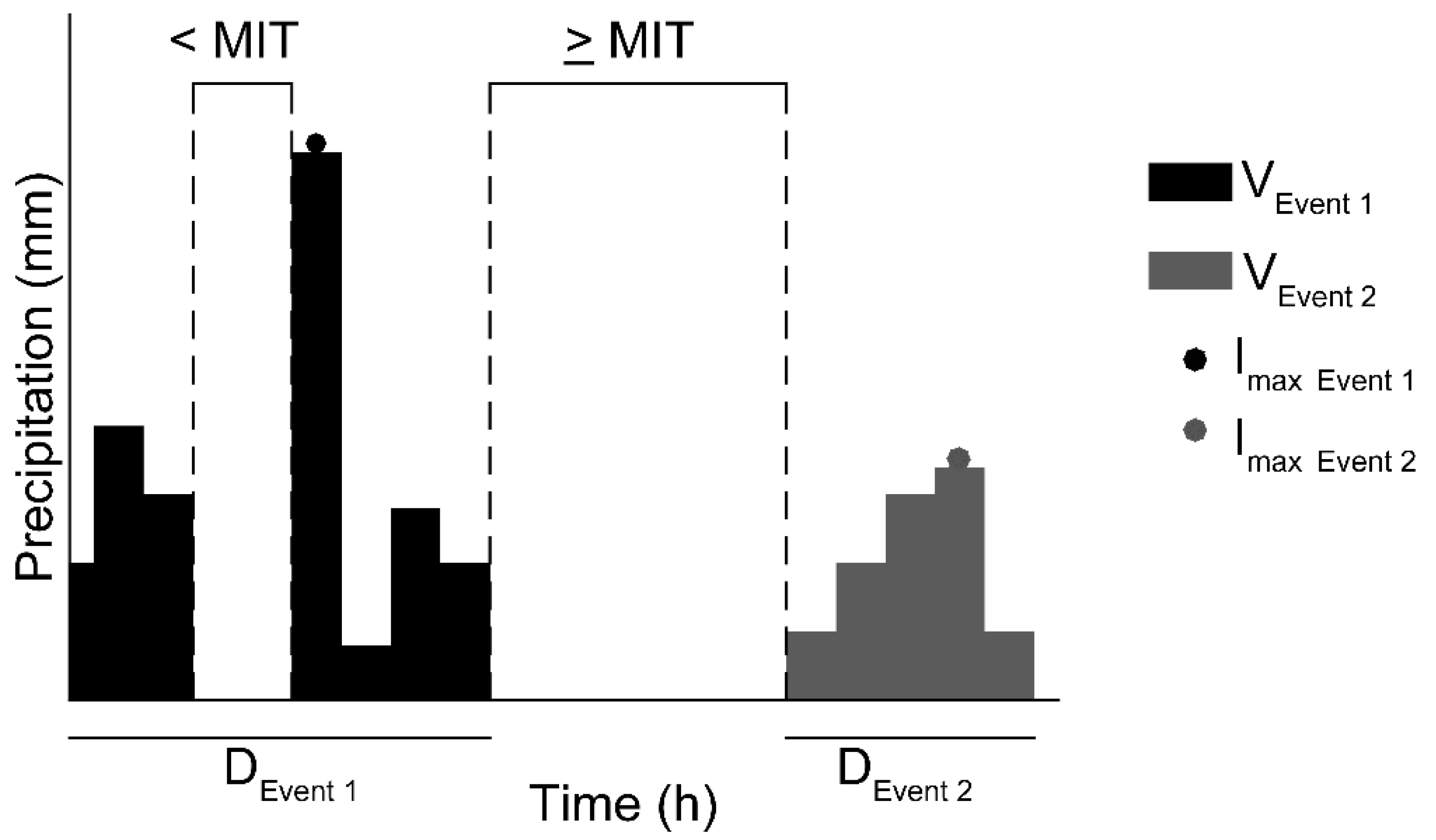
• Storm events separation and rank. Analyzing the rainfall series within the stochastic weather series generated, we separated the independent storm events applying the exponential method [31]. Afterwards we ranked each storm within its year of occurrence following three main criteria: Total rainfall depth, maximum intensity, and total duration.
• Rainfall versus flood comparison. We obtained the flood hydrograph related to each storm event. We analyzed the relationship between the storm rank and (a) the maximum annual peak-flow and maximum annual volume, (b) the seasonality of flood hydrographs, (c) the dependence between the peak-flow and volume, and (d) the bivariate frequency of floods through a copula-based analysis.

2.1. Stochastic Weather Forcing. AWE-GEN: The Advanced WEather GENerator

AWE-GEN [30] is a generator capable of reproducing low and high-frequency characteristics of hydro-climatic variables and essential statistical properties of these variables. The weather generator employs both the physically-based and stochastic approaches and is a substantial evolution of the model presented by Ivanov et al. [32]. AWE-GEN is a statistical hourly stationary model capable of reproducing statistical properties of several weather variables including precipitation, cloud cover, shortwave incoming radiation, air temperature, vapor pressure, wind speed, and atmospheric pressure over a range of time scales. Since rainfall is the main weather variable involved in the framework of this work, a brief introduction of the precipitation model is reported. Furthermore, a brief summary of the air temperature model is reported due to its importance in the weather generation process.

The AWE-GEN uses the point Neyman–Scott rectangular pulse approach to generate the internal structure of the precipitation process, based on Cowpertwait [33] studies. Such models are able to capture the main observed rainfall time-series statistic characteristics; for the case of the AWE-GEN model: (1) Mean waiting time between adjacent storm origins (h); (2) mean waiting time for rain cell origins after the storm origin (h); (3) mean duration of the rain cell (h); (4) mean number of cells per storm (-); (5) shape parameter (-) and (6) scale parameter (mm/h) of the Gamma distribution of rainfall intensity. These six parameters are fitted minimizing an imposed objective function using the simplex method [34] on a monthly basis, i.e., the six parameters are inferred for each month in order to account for seasonality.

As exposed by Fatichi et al. [30], to validate the generated series it is recommendable to analyze statistics different from those used in the calibration. Within this paper, as the focus is on rainfall events and floods, we analyzed how the stochastic generated series were able to reproduce the observed rainfall extreme properties.

With regard to the air temperature model, AWE-GEN generates the air temperature series using a stochastic physic-based approach developed by Ivanov et al. [32]. This model is able to reproduce the intra-daily variation of air temperature. In particular, the temperature at a generic time is obtained as the sum of a deterministic and a stochastic component. The deterministic component is assumed to be directly related to the divergence of eddy and radiative heat fluxes, whereas the stochastic component is estimated through an autoregressive model. The air temperature model uses parameters and coefficients estimated at a monthly scale.

The reader is referred to Fatichi et al. [30] and Ivanov et al. [32] for further details on AWE-GEN.

2.2. Hydrological Simulations. tRIBS: The TIN-based Real-Time Integrated Basin Simulator

As exposed, we used tRIBS [29,30] to perform the hydrological simulations. tRIBS is a physically based, distributed continuous hydrologic model. Its predecessor, the real-time integrated basin simulator (RIBS) of Garrote and Bras [35] implemented an event-based model for rainfall–runoff analysis. tRIBS has inherited the functionality of RIBS while adding the hydrology necessary for continuous operation. tRIBS uses an adaptive multiple resolution approach, described by Vivoni et al. [36], based on triangulated irregular networks (TIN) to represent the terrain topography. tRIBS considers the spatial variability in precipitation fields, land-surface descriptors, and is able to solve the basin hydrologic response at an hourly temporal resolution and a very fine spatial (10–100 m) scale. tRIBS includes parameterizations of rainfall interception, evapotranspiration, infiltration with continuous soil moisture accounting, lateral moisture transfers in the unsaturated and saturated zones, and kinematic-wave runoff routing.

The model computational basis, structure, and description of process parameterizations are given in full detail in [29,30].

2.3. Storm Events Separation. The Exponential Method and Rank of Storm Events

2.3.1. The Exponential Method

There are different methodologies [31,37,38,39] to identify independent rainfall events. Rain events are usually identified by fixing the duration of the minimum inter-event time (MIT) that follows, or precedes, a rainfall event. Two rainfall events are independent if there is no rainfall (considering a minimum rainfall threshold of 0.25 mm/h) between them in a period equal or superior to the MIT (Figure 2).

Within this study, we applied the exponential method [31] to determine the value of the MIT. This method assumes that the storm arrival time and the time between two storms follows an exponential distribution. Consequently, the duration of dry periods can be approximated by an exponential distribution with a mean that is equal to the standard deviation, and therefore the coefficient of variation (CV) is equal to one.

To obtain the value of the MIT, we obtained the CV for different dry-period durations applying Equation (1):

$$\mathrm{C}{\mathrm{V}}_{\mathrm{k}}=\mathrm{std}\left({\mathrm{dp}}_{\mathrm{k}}\right)/\overline{\mathrm{d}{\mathrm{p}}_{\mathrm{k}}},$$

(1)

where k is the dry-period duration (1 h, 2 h, …), $\overline{\mathrm{dp}}$_k is the average of dry-period durations greater than the duration of kth, and std(dp_k) its standard deviation. The value of the MIT is determined as the value of k in which CV_k approximates to one.

Once we obtained the MIT, we separated all the storm events within the rainfall time-series. We did the separation to the observed and generated series for: (a) The validation of AWE-GEN simulations, and (b) for the comparison of rainfall versus floods.

2.3.2. Rank of Storm Events

Analyzing all the separated storm events, we ranked them according to three criteria: Total depth (V_Event), maximum intensity (I_max), and duration (D_Event) (Figure 2). We ranked the events in the 5000 years within the same year from the highest to the lowest according to the three criteria. Therefore, for each criterion, the biggest rainfall event of each year was identified as rank one, the second one as rank two, etc.

Finally, for each criterion, we identified the rank of the storm event (maximum intensity, total depth, and total duration) that generated the maximum peak-flow and maximum flood volume of each year within the 5000-year time-series.

2.4. Rainfall versus Flood Comparison

We analyzed what the maximum rank of a storm event is that should be considered to preserve the properties of extreme floods regarding: (a) Magnitude and recurrence (univariate frequency analysis), (b) seasonality, (c) dependence of maximum annual peak-flows and volumes and (d) bivariate magnitude and recurrence (copula-based frequency analysis).

In several sections within this manuscript, in order to compare the values obtained at the different ranks to the reference value (the one obtained from the continuous simulation), we obtained the relative error (RE) as follows (Equation (2)):

$$\mathrm{RE}(\%)=\left(1-\frac{\mathrm{Compared}\mathrm{value}}{\mathrm{Reference}\mathrm{value}}\right)·100,$$

(2)

2.4.1. Magnitude and Recurrence. Univariate Frequency Analysis

We analyzed how the storm events were related to the maximum annual peak-flow and volume focusing on the:

• Probability that a storm with a determined rank generates the maximum annual value of the (a) peak-flow and (b) volume.
• Relation between the storm rank and the return period associated to the (a) maximum annual peak-flow and (b) maximum annual volume.
• Maximum storm rank required to obtain 95% and 99% probability of achieving the (a) maximum peak-flow and (b) maximum volume for a specific year and for different ranges of the return period.

We assigned the return periods to the maximum annual peak-flows and to the maximum annual volumes independently, by using the Gringorten plotting position formula [40].

2.4.2. Seasonality

We carried out a seasonality analysis based on circular statistics [41]. We analyzed how the seasonality of the maximum annual peak-flows and volumes is affected by the rank of storms.

As exposed by [42], circular statistics are an effective method to define the basis of the timing of hydrological extreme events within a year. The date of occurrence of an event in year i can be graphed on a unitary circle to give the angle (θ_i) in polar coordinates (Equation (3)):

$${\mathsf{\theta }}_{\mathrm{i}}=\mathrm{D}·2\mathsf{\pi }/\mathrm{L},$$

(3)

where D stands for the day of the year (one for 1 January, two for 2 January, etc.) and L the number of days within the year (365, or 366 if it is a leap year). Then, the mean seasonality can be defined as the average vector from the origin which represents the mean date of occurrence ($\overline{\mathsf{\theta }}$) of all the maximum annual floods (peak-flow or volume) within the case study basin. The $\overline{\mathrm{x}}$ and $\overline{\mathrm{y}}$ coordinates of the average vector are obtained from the sample of 5000 extreme events by (Equations (4) and (5)):

$$\overline{\mathrm{x}}=\frac{{{\displaystyle \sum }}_{\mathrm{i}=1}^{\mathrm{5,000}}\cos \left({\mathsf{\theta }}_{\mathrm{i}}\right)}{\mathrm{5,000}},$$

(4)

$$\overline{\mathrm{y}}=\frac{{{\displaystyle \sum }}_{\mathrm{i}=1}^{\mathrm{5,000}}\sin \left({\mathsf{\theta }}_{\mathrm{i}}\right)}{\mathrm{5,000}},$$

(5)

therefore (Equation (6)):

$$\overline{\mathsf{\theta }}={\tan }^{-1}\frac{\overline{\mathrm{y}}}{\overline{\mathrm{x}}},$$

(6)

whereas the variability of the date of occurrence about the mean date is characterized by the length parameter $\overline{\mathrm{r}}$ (Equation (7)):

$$\overline{\mathrm{r}}=\sqrt{{\overline{\mathrm{x}}}^2+{\overline{\mathrm{y}}}^2},$$

(7)

which ranges from zero (uniform distribution around the year) to one (all extreme events occur on the same date of the year).

We compared the values of $\overline{\mathsf{\theta }}$ and $\overline{\mathrm{r}}$ obtained from the continuous simulation to those obtained from the different storm ranks.

2.4.3. Dependence

We measured and analyzed how the different storm ranks affected the dependence between the peak-flow and volume. To do so, we used (1) graphical techniques and (2) numerical measures.

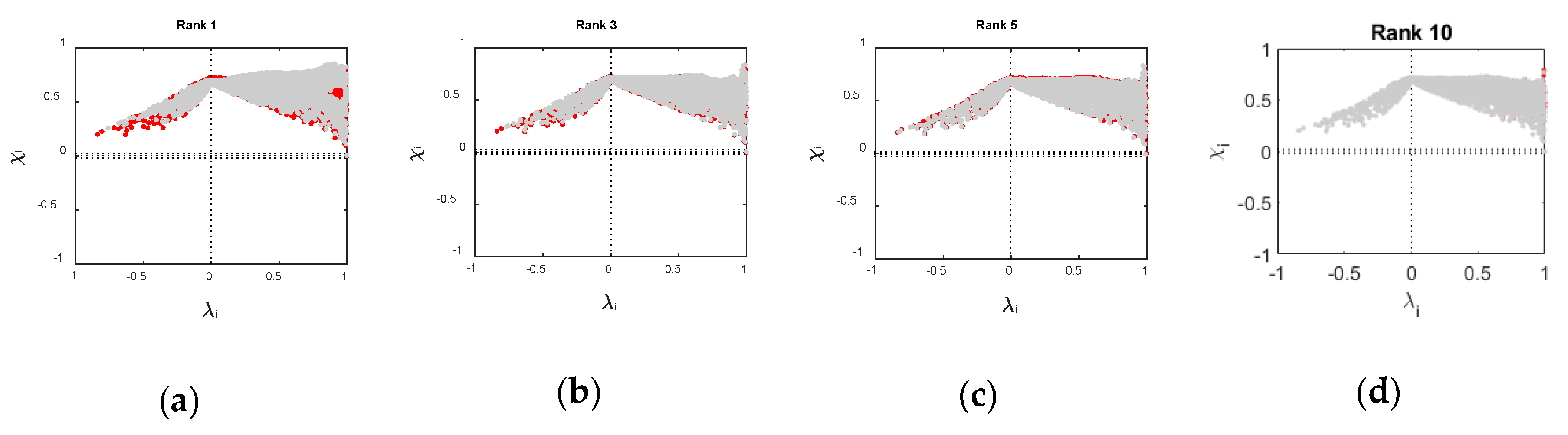
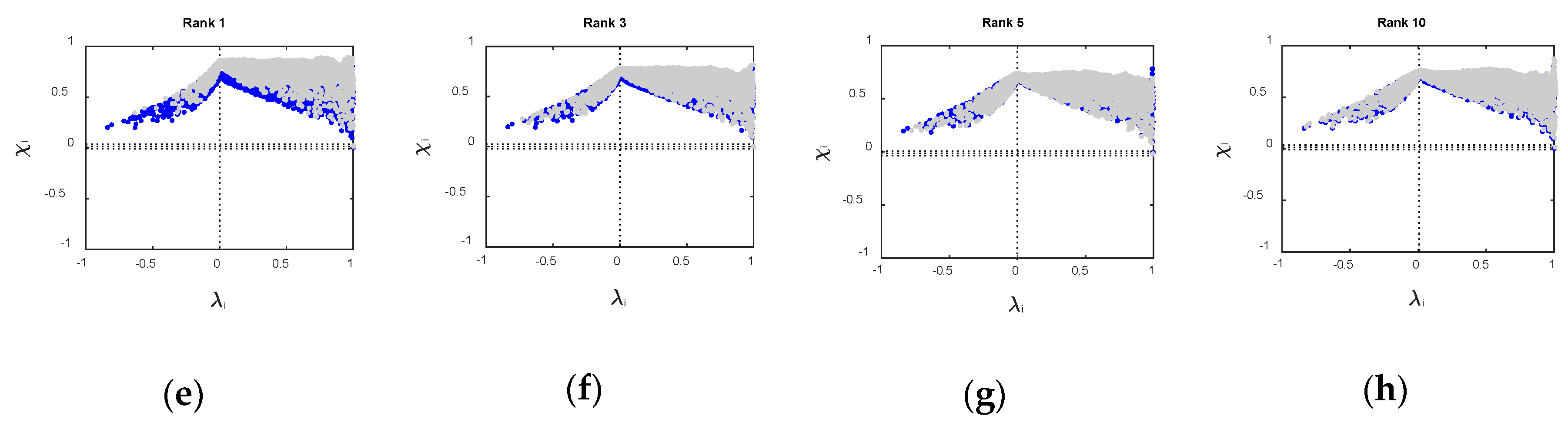
• We graphed the Chi-Plot, which is a technique that displays a measure of location of an observation regarding the whole of the observations (λ_i) against a measure of the Chi-square test statistic for independence (Χi). Therefore, the bigger the distance between the points and the horizontal axis is, the larger the dependence is. The dependence is positive if the points are above the upper control limit, and negative if they are located below the lower control limit [43,44], which we established with a probability of 90% as shown in Genest et al. [45].
• Spearman’s rho and Kendall’s tau. Moreover, dependence measures are needed to procure a quantitative value of the dependence relation between variables. For this purpose, we adopted the Spearman’s rho and Kendall’s tau as rank-based non-parametric measures of dependence.

2.4.4. Magnitude and Recurrence. Copula-based Frequency Analysis.

Finally, we analyzed how the rank of storms affected the bivariate properties of the pairs of peak-flow and volume by carrying out a copula-based analysis. To do so, we used the MATLAB toolbox MhAST Toolbox [46]. Within that toolbox, a total of 26 parametric models of copula families can be fitted to bivariate data. Within this study, for the sake of simplicity, we focused on three well-known Archimedean one-parameter copula families for their uses in hydrological sciences: Clayton, Gumbel and Frank. We proceeded as follows:

First, we fitted the three studied copulas to the pairs peak-flow and volume values obtained from the continuous simulation using MhAST. For these three copulas, MhAST uses the MATLAB built-in function, which estimates the parameter (${\mathsf{\theta }}_{\mathrm{c}}$) of each copula using the method of maximum likelihood. To select the copula that provided the best fit, we analyzed the root mean square error (RMSE) (Equation (8)) and the Nash–Sutcliffe efficiency (NSE) (Equation (9)) coefficient, which measures how different the empirical observed bivariate probabilities ($\tilde{\mathrm{Y}}$) and their modelled bivariate counterpart (Y) are:

$$\mathrm{RMSE}=\sqrt{\frac{{{\displaystyle \sum }}_{\mathrm{i}=1}^{\mathrm{n}}{\left[{\tilde{\mathrm{y}}}_{\mathrm{i}}-{\mathrm{y}}_{\mathrm{i}}\left({\mathsf{\theta }}_{\mathrm{c}}\right)\right]}^2}{\mathrm{n}}},$$

(8)

$$\mathrm{NSE}=1-\frac{{{\displaystyle \sum }}_{\mathrm{i}=1}^{\mathrm{n}}{\left[{\tilde{\mathrm{y}}}_{\mathrm{i}}-{\mathrm{y}}_{\mathrm{i}}\left({\mathsf{\theta }}_{\mathrm{c}}\right)\right]}^2}{{{\displaystyle \sum }}_{\mathrm{i}=1}^{\mathrm{n}}{\left[{\tilde{\mathrm{y}}}_{\mathrm{i}}-\overline{{\tilde{\mathrm{y}}}_{\mathrm{i}}}\right]}^2},$$

(9)

RMSE values are within the range [0, ∞) with zero being a perfect fit, whereas NSE ranges in the interval (−∞,1], with one being the perfect fit. The best fit is the one that had a lower value of RMSE and a higher value of NSE.

Once the copula family was chosen, we fitted that copula to the different pairs of peak-flow and volume obtained considering different storm ranks, according to the rainfall criteria separation studied. We obtained the RE of the estimated copula parameter with respect to the copula parameter of the continuous simulation.

Finally, we graphically analyzed the differences between the Kendall’s return period (T_K) [47] calculated by both, continuous simulation and different storm ranks according to the V_Event and I_max criteria. Kendall’s return period represents the mean inter-arrival time of critical events lying on the probability level t, and can be obtained as follows (Equation (10)):

$${\mathrm{T}}_{\mathrm{K}}=\frac{\mathsf{\mu }}{1-{\mathrm{K}}_{\mathrm{C}}\left(\mathrm{t}\right)}=\frac{1}{1-{\mathrm{K}}_{\mathrm{C}}\left(\mathrm{t}\right)},$$

(10)

where μ is the average interarrival time of events (i.e., μ = 1 in this paper, as annual maxima are being analyzed) and K_C(t) is the Kendall’s distribution function, where t represents the probability level. For the sake of brevity, the reader is referred to [47,48] for further details. We obtained the isolines of T_K of 10, 50, and 100 years estimated through continuous simulation and through different storm ranks for the studied criteria separation using the MhAST toolbox.

2.5. Case Study

2.5.1. Study Basin

The methodology was applied in Peacheater Creek (herein, PC), using the hourly climate data of Westville, a weather station located within the basin (Figure 3a).

This sub-basin is located in Baron Fork at Eldon river basin (Oklahoma, USA) and it was selected since it was originally used to test, calibrate, and validate the tRIBS model [29,48]. The Peacheater Creek basin has a drainage area of 64 km², with elevations ranging between 248 and 432 m.a.s.l. The sub-basin is characterized by gentle (slopes between 2% and 5%) to steep (slopes between 15% and 40%) hillslopes. The vegetation is a mixture of oak-hickory-pine forest grasslands (mainly located in the southern part of the basin) and cropland-urban areas (mainly in the northern region). The impervious fraction of the sub-basin is estimated to be about 1.56%. The predominant soil consists of gravelly silt loams [29].

Additional details on the climate, hydrology, and basin characteristics have been presented in [29,30,49].

2.5.2. Setup of Modeling Experiments

Two different modeling experiments were carried out:

• Stochastic weather generation: We generated 5000 years of punctual hourly weather with AWE-GEN [28], calibrated with the climate data recorded from 1997 to 2016 (both years included) at the Westville weather station: Rainfall, temperature, wind speed, radiation, cloudiness, relative humidity, and atmospheric pressure. Raw data had a resolution of 5 min. We processed the data into hourly values, in order to force AWE-GEN and perform the stochastic weather generation.
• Hydrological simulations: Numerical simulations in PC were carried out using the tRIBS model with a TIN of 6680 nodes (Figure 3b) derived from a US Geological Survey (USGS) 30-m DEM using the procedure described in Vivoni et al. [36]. We based our simulations on a model calibration conducted by Ivanov et al. [29,49] as part of the distributed model intercomparison project. Ivanov et al. [49] obtained a correlation coefficient of 0.763 and a Nash-Sutcliffe coefficient of 0.565 (which can be considered as satisfactory following the guidelines exposed in Sirisena et al. [50]) for the hourly simulated streamflow at the outlet of Baron Fork basin (in which PC is located), compared to the hourly observed streamflow from April of 1994 to July of 2000. To make the experiment approachable, the computational load was balanced by using parallel computing techniques. The basin was partitioned into eight different parts using a surface-flow partitioning script [5] with the graph-partitioning software METIS [51], which balances the number of TIN nodes across processors minimizing the dissections that occur in the channel network. Each processor calculates tRIBS variables within each part of the basin and, every time step each processor sends messages to the others to sum up all the calculations done within the basin. Thus, the computational load is balanced between the different processors (Figure 3c) and the experiment is approachable.

The experiment was carried out by using Magerit, a high performance computer owned by the Technical University of Madrid. We used the Intel family processors architecture, which consists of 41 nodes with two intel processors Intel XEON E5-2670 of eight cores each, and 64 GB RAM/Core. The time spent in the hydrological simulations was two and a half months, whilst the weather simulations were carried out within one day of computation.

2.6. Limitations of the Methodology

The proposed methodology has some limitations that should be noted:

• Rainfall was considered uniform within the whole basin, as a result of using a punctual stochastic weather generator. As pointed out by Liuzzo et al. [8], due to the small size of PC, there is not a big difference between considering the spatial and punctual rainfall. However, within the same study, accounting or not for the rainfall spatially had an appreciable difference for a basin with a bigger drainage area (Baron Fork, 808 km²).
• The study is focused on return periods up to 500 years. For higher return periods, the length of the generated weather forcing series should be analyzed to ensure that it is representative enough of the return period studied.
• The procedure did not account for climate-change effects or land-use changes, but considered stationary climate conditions. However, interannual variations of the mean annual rainfall were accounted for due to the nature of AWE-GEN.
• The methodology is applied to one basin, which limits the extrapolation of the results obtained.

3. Results and Discussion

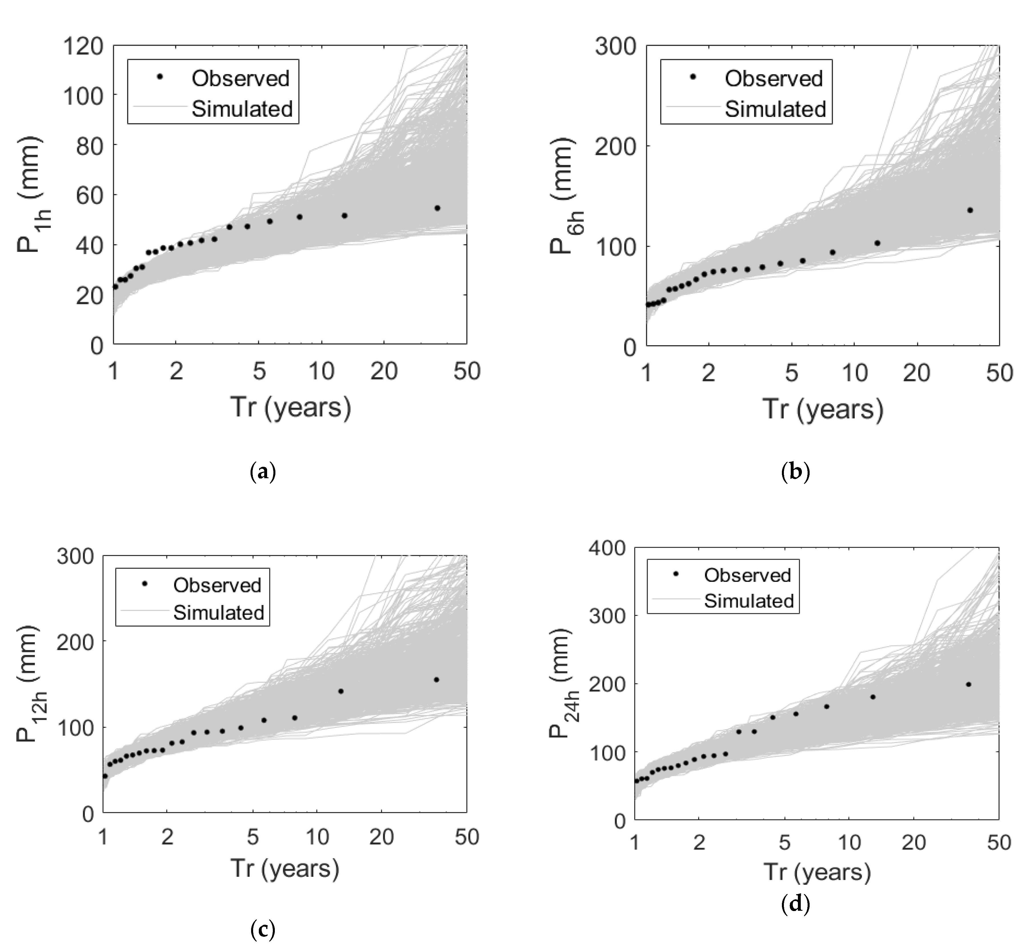
3.1. Stochastic Weather Generation. Rainfall Extremes Validation.

We analyzed the ability of the weather generator (AWE-GEN) to reproduce rainfall extremes by comparing the stochastic rainfall frequency curves with those observed at different aggregation periods (Figure 4a–d, 1 h, 6 h, 12 h, 24 h, respectively). As shown, the behavior of the observed rainfall frequency curves was mostly within the range of the simulated ones.

Furthermore, we analyzed if the seasonality of the storm events was retained by AWE-GEN. To carry out the analysis, it was necessary to separate the storm events. By applying the exponential method (exposed in Section 2.3.1) we determined a MIT of 15 h from the observed hourly rainfall time-series of Westville Station.

Applying the methods shown in Section 2.4.2, we compared the seasonality of two main characteristics of storm events (Figure 2): The maximum annual I_max (Figure 4e) and the maximum annual V_Event (Figure 4f). The seasonality is well-reproduced by AWE-GEN for the maximum annual I_max (Figure 4e). The mean occurrence ($\overline{\mathsf{\theta }}$) (represented by the direction of the vectors) is late June (observed, in blue) and early July (simulated, in black), with a similar variability of seasonality ($\overline{\mathrm{r}}$) (represented by the length of the vectors (Figure 4e)), with an observed and simulated value of 0.61 and 0.56, respectively). However, in the case of V_Max (Figure 4f), the observed seasonality is slightly more disperse than the generated (the length of the observed vector is 0.16, whereas the simulated is 0.29) and $\overline{\mathsf{\theta }}$is delayed by one month. Overall, the generated synthetic series are able to reproduce extreme rainfall properties.

3.2. Rainfall versus Flood Comparison.

Once the weather series had been generated, we used them as weather forcing for the hydrological model tRIBS and performed the simulations. Afterwards, we obtained the relationship between the storm ranks and the flood hydrographs generated at the basin outlet.

3.2.1. Magnitude and Recurrence. Univariate Frequency Analysis

Table 1. Relative and cumulated frequency that a storm of a specific rank generates the maximum annual peak-flow and the maximum annual volume.

Storm Rank	Relative/Cumulated Frequency of Coincidence with Maximum Annual Peak-Flow (%)			Relative/Cumulated Frequency of Coincidence with Maximum Annual Volume (%)
	Total Depth	Maximum Intensity	Total Duration	Total Depth	Maximum Intensity	Total Duration
1	53.5/53.5	45.2/45.2	9/9	68.8/68.8	35.6/35.6	17.2/17.2
2	21.7/75.2	18.6/63.8	5.8/14.8	17.9/86.7	17.3/52.9	8.6/25.9
3	11.4/86.6	11.5/75.3	4.8/19.6	6.9/93.6	11.3/64.2	7/32.9
4	5.3/91.9	6.9/82.2	3.3/22.9	2.7/96.3	8/72.2	4.7/37.5
5	3.4/95.3	4.2/86.4	3.6/26.5	1.8/98.1	5.5/77.7	4.5/42
6	1.7/97	3.1/89.4	2.9/29.5	0.7/98.8	4.2/81.9	3.4/45.4
7	1.3/98.2	2.2/91.7	2.9/32.3	0.5/99.3	3.1/85	3/48.4
8	0.8/99	2.1/93.7	2.5/34.8	0.3/99.6	2.8/87.9	3/51.4
9	0.3/99.3	1.5/95.2	2.3/37.1	0.1/99.7	2.5/90.4	2.4/53.8
≥10	0.7/100	4.8/100	62.9/100	0.3/100	9.6/100	46.2/100

shows the probability that a storm of a specific rank generates the (a) maximum annual peak-flow and (b) the maximum annual volume. The three ranking criteria are shown: V_Event, I_max, and D_Event. It can be seen that the V_Event criteria was the most relevant; that is, a lower storm rank is required for obtaining both the maximum annual peak-flow and volume.

According to the different storm rank criteria:

• V_Event. Considering the biggest storm (rank one) results in a probability of generating the maximum annual peak-flow (Table 1) of more than 53%, whereas considering the storms of rank one and two this probability increases to more than 75%. If the storms considered are up to rank 3, this probability exceeds 86%. When analyzing the maximum annual volume (Table 1), the same probabilities are greater than 68%, 86%, and 93%, respectively.
• I_max. The probability of generating the maximum annual peak-flow (Table 1) is more than 45%, 63%, and 75% for a storm rank up to one, two, and three, respectively. In the case of maximum annual volume (Table 1), the same Figures are 35%, 52%, and 64%.
• D_Event. The probability of achieving the maximum annual peak-flow and volume with these criteria is the lowest. Considering storms up to rank ten, the probability of achieving the maximum peak-flow is less than 40% (Table 1), and less than a 60% (Table 1) probability of resulting in the maximum annual volume.

Therefore, for PC, the best criterion of the storm rank is V_Event, followed up by I_max when analyzing the correspondence between the storms and maximum annual peak-flow and volume. For the sake of simplicity, the following results only focused on these two criteria, excluding D_Event.

Afterwards, we focused on the magnitude of peak-flows and volumes. We related the different storm ranks (Figure 5, total depth criteria (red) maximum intensity criteria (blue)) to the associated return period (Tr) of peak-flows (Figure 5a) and volumes (Figure 5b) obtained from the analysis of the 5000 years flow simulated at the basin outlet. According to the two criteria selected, it can be seen that:

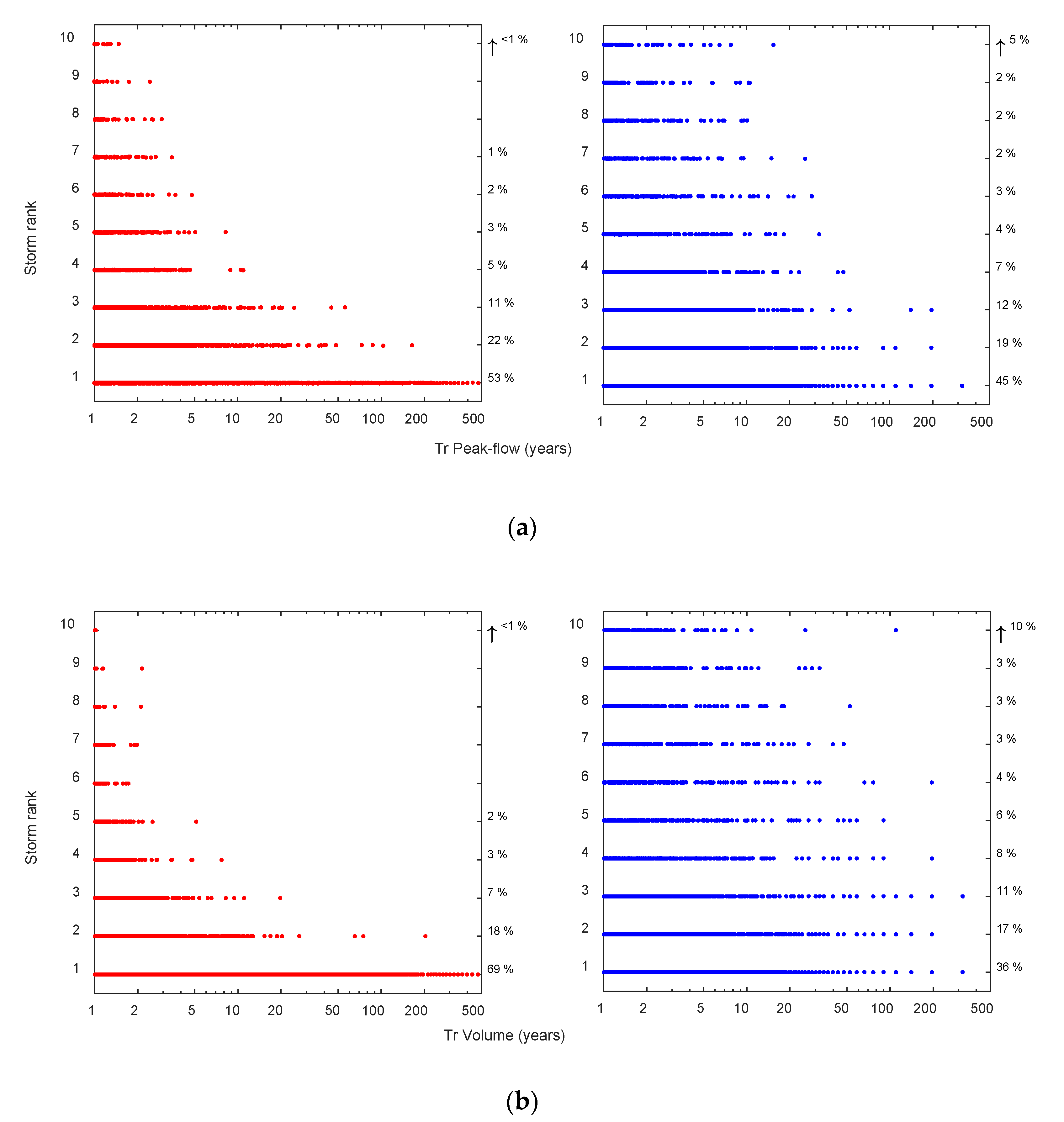
• V_Event. The higher the Tr of the peak-flow (Figure 5a) and volume (Figure 5b) are, the lower the storm rank needed. Therefore, there is a strong correlation between the Tr and the storm rank. For the Tr of the peak-flow over 10 years, all the storm events have a rank lower than or equal to four, whereas for the Tr over 100 years all the storms are of rank one or two. For the Tr of volume over 10 years, all the storm events have a rank lower than or equal to three, whereas for the return periods over 100 years all the storms are also of rank one or two.
• I_max. There is more dispersion than in the V_Event criteria. For the Tr of the peak-flow over 10 years, storms have a rank of ten or lower, whereas for the Tr over 100 years all the storms up to rank three should be considered. In the case of volume, the Tr higher than 10 years corresponds to storms with ranks up to 23 (not shown in Figure 5), whereas for the Tr over 100 years, storms up to rank ten can generate the maximum annual volume.

Finally, regarding the analysis of magnitude and recurrence, we calculated the maximum storm rank required to obtain 95% and 99% probability of achieving the maximum annual peak-flow and the maximum annual volume for a specific year and for different ranges of Tr for the V_Event and I_Max criteria (

Table 2. Maximum storm rank required to obtain 95% and 99% probability of achieving the maximum peak-flow or volume for a specific year, depending on the ranking criteria used and the range of return periods studied.

Probability (%)	Tr (Years)	Maximum Storm Rank to be Considered Peak-Flow		Maximum Storm Rank to be Considered Volume
		Total Depth	Maximum Intensity	Total Depth	Maximum Intensity
95/99	All range	5/8	9/16	4/7	13/22
95/99	1 ≤ Tr < 10	6/9	10/16	4/7	13/22
95/99	10 ≤ Tr < 50	3/3	4/7	1/2	8/14
95/99	50 ≤ Tr < 100	2/3	2/3	1/2	6/10
95/99	Tr ≥ 100	2/2	2/3	1/2	6/6

). Considering storms up to rank six according to the V_Event criteria, there is a 95% probability of achieving the maximum annual peak-flow and volume for all ranges of the Tr, which increases to 99% if all storm events up to rank nine are considered. For I_Max, the ranks are 13 and 22 for the same probability values. As also shown in Figure 5, the storm rank required is less as the Tr increases in the two ranking criteria. It is remarkable that, in the case of V_Event, for return periods higher than 50 there is a probability of achieving the maximum annual peak-flow and the maximum annual volume of 99% if the three highest events are considered.

3.2.2. Seasonality

We studied if seasonality was preserved by the storms depending on the rank considered. Figure 6 shows the seasonal behavior of storms regarding the maximum peak-flow (Figure 6a–d and Figure 6i–l) and maximum volume (Figure 6e–f and Figure 6m–p). Comparisons were carried out with the seasonality of the continuous simulation (red in Figure 6a–f and blue in Figure 6i–p) and the consideration of storms up to rank one, three, five and ten for the V_Event (Figure 6a–f) and I_Max (Figure 6i–p) criteria.

According to the two rainfall criteria selected:

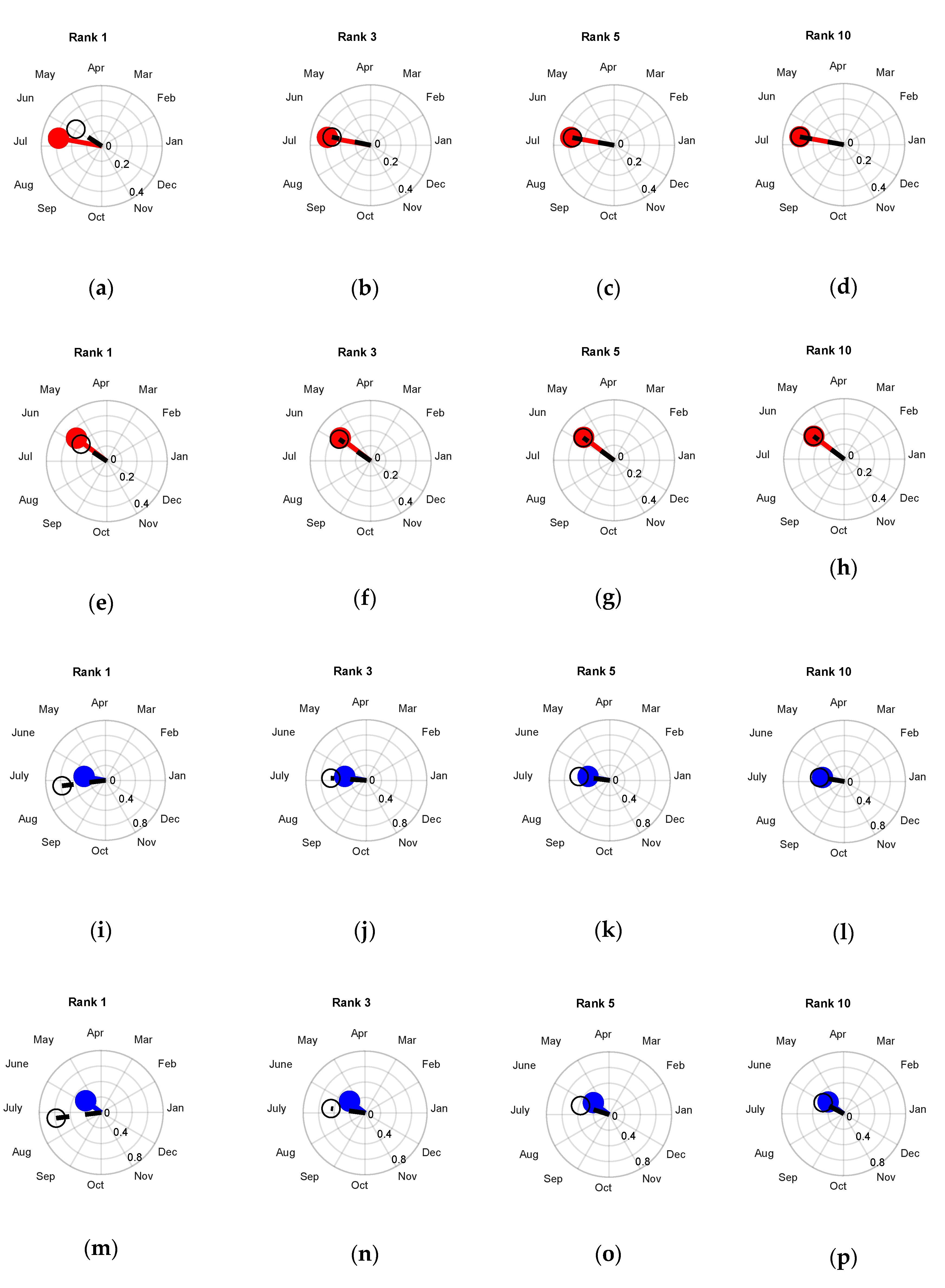
• V_Event. The seasonality is preserved almost equally if storms are at least considered up to rank three for both the maximum peak-flow and maximum volume.
• I_Max. Within this case, to preserve the seasonality obtained from the continuous simulation, storms up to rank ten should be considered in both cases, the maximum peak-flow and maximum volume.

To quantify the impact of the rank of storms in seasonality, we obtained the values of $\overline{\mathsf{\theta }}$ and $\overline{\mathrm{r}}$ from the continuous simulation and compared them to the ones obtained from the different storm ranks, obtaining the RE (Equation (2)).

Table 3. Seasonality of the maximum annual peak-flow represented by the angle of its mean direction ($\overline{\mathsf{\theta }}$ ) and its radio ($\overline{\mathrm{r}}$ ), for different storm ranks and for the two different criteria studied. The relative error (RE) is also shown.

Maximum Storm Rank Considered	Total Depth		Maximum Intensity		Total Depth		Maximum Intensity
	$\overline{\mathsf{\theta }}$	$\overline{\mathbf{r}}$	$\overline{\mathsf{\theta }}$	$\overline{\mathbf{r}}$	$\mathbf{R}{\mathbf{E}}_{\overline{\mathsf{\theta }}}$	$\mathbf{R}{\mathbf{E}}_{\overline{\mathbf{r}}}$	$\mathbf{R}{\mathbf{E}}_{\overline{\mathsf{\theta }}}$	$\mathbf{R}{\mathbf{E}}_{\overline{\mathbf{r}}}$
Continuous Simulation	169.7	0.29	169.7	0.29	−	−	−	−
Rank 1	146.7	0.20	187.2	0.59	13.5	29.8	−10.3	−101
Rank 3	168.1	0.26	176.5	0.47	0.9	10.1	−4.0	−61.5
Rank 5	169.7	0.28	173.0	0.41	0.0	3.8	−2.0	−40.4
Rank 10	169.9	0.29	170.9	0.33	−0.1	0.0	−0.7	413.1

and

Table 4. Seasonality of the maximum annual volume represented by the angle of its mean direction ($\overline{\mathsf{\theta }}$ ) and its radio ($\overline{\mathrm{r}}$ ), for different storm ranks and for the two different criteria studied. The relative error (RE) is also shown.

Maximum Storm Rank Considered	Total Depth		Maximum Intensity		Total Depth		Maximum Intensity
	$\overline{\mathsf{\theta }}$	$\overline{\mathbf{r}}$	$\overline{\mathsf{\theta }}$	$\overline{\mathbf{r}}$	$\mathbf{R}{\mathbf{E}}_{\overline{\mathsf{\theta }}}$	$\mathbf{R}{\mathbf{E}}_{\overline{\mathbf{r}}}$	$\mathbf{R}{\mathbf{E}}_{\overline{\mathsf{\theta }}}$	$\mathbf{R}{\mathbf{E}}_{\overline{\mathbf{r}}}$
Continuous Simulation	142.9	0.25	142.9	0.25	−	−	−	−
Rank 1	146.7	0.20	187.2	0.59	−2.7	18.9	−31.0	−133
Rank 3	145.4	0.25	172.7	0.44	−1.7	−0.3	−20.8	−76.1
Rank 5	143.7	0.25	162.7	0.38	−0.6	−0.6	−13.8	−51.6
Rank 10	143.2	0.25	151.8	0.30	−0.2	−0.6	−6.2	−20.0

show the different values of $\overline{\mathsf{\theta }}$ and $\overline{\mathrm{r}}$ depending on the criteria and the RE, for the maximum peak-flow (Table 3) and for maximum volume (Table 4). According to the two rank criteria:

• VEvent. With storms up to rank five, there is less than 1% absolute RE in the estimation of the mean direction of seasonality for both the peak-flow (Table 3) and volume (Table 4). Regarding the radius, which measures the dispersion of the seasonality, considering storms up to rank five have an absolute RE lower than 4%.
• IMax. With this criterion, the smaller absolute values of RE are in the estimation of the mean direction of the maximum peak-flow seasonality (2% if storms up to rank five are considered). When analyzing the mean direction of volume seasonality, RE is over 6% for storms up to rank ten. When it comes to the radio, all RE values are over 10%.

Therefore, the V_Event sorting criterion is the best for preserving the seasonality of floods in this case study.

3.2.3. Dependence

We analyzed how the storm ranks are able to preserve the dependence between the peak-flow and volume of the continuous simulation. To do so, as exposed in the methodology, we graphed the chi-plots comparing the peak-flow volume dependence from the continuous simulation (red (Figure 7a–d) and blue (Figure 7e–h) dots) to the different storm ranks according to the V_Event and I_Max criteria (grey dots in Figure 7).

For all cases (Figure 7), there is a positive dependence between the peak-flow and volume. Furthermore, when focusing on the upper tail dependence (first quadrant within all the plots in Figure 7), the points are located far from the zero value of the y axis, which is the independence hypothesis. Depending on the criteria:

• V_Event. The dependence is well preserved, and both scatterplots are visually almost identical when the storm ranks up to three or more are considered. If the biggest storm of the year is considered, the dispersion is bigger.
• I_max. Dependence is also preserved for this criterion, but a higher dispersion is shown in rank periods up to one and three. In the case of considering only the biggest storm (rank one), a big dispersion is found in the upper tail.

To numerically compare the degree of dependence of the peak-flow and volume of the continuous simulation with respect to different storm ranks, values of Spearman’s rho and Kendall’s tau were computed (

Table 5. Rank-based non-parametric measures of dependence Spearman’s rho (ρ) and Kendall’s tau (τ) for the pair of values of maximum annual peak-flows and maximum annual volumes regarding the maximum storm rank considered and to the criteria used: Total depth or maximum intensity.

Maximum Storm Rank Considered	Total Depth		Maximum Intensity		Total Depth		Maximum Intensity
	ρ	τ	ρ	Τ	REρ	REτ	REρ	REτ
Continuous Simulation	0.884	0.709	0.884	0.709	−	-	−	−
Rank 1	0.883	0.708	0.955	0.826	0.07	0.01	−8.05	−16.56
Rank 3	0.882	0.706	0.922	0.767	0.17	0.31	−4.26	−8.18
Rank 5	0.883	0.708	0.903	0.739	0.05	0.05	−2.16	−4.27
Rank 10	0.884	0.709	0.888	0.716	0.00	−0.01	−0.41	−1.01

), and their RE (Equation (2)). In the case of the V_Event criterion, all the absolute values of RE obtained from the different ranks are lower than 1%, whereas in the case of I_max, the absolute RE values are over 2% for storms up to rank five, reaching absolute RE values of less than 1% if only storms up to rank ten are considered.

Therefore, to preserve the dependence between maximum annual peak-flows and volumes, V_Event is also the best criteria for the case study.

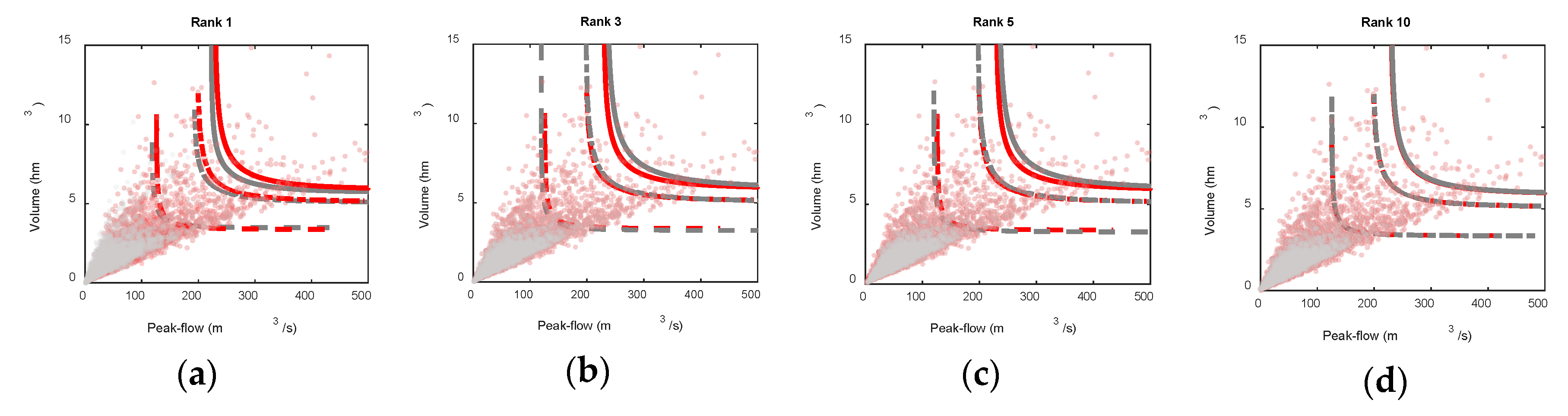
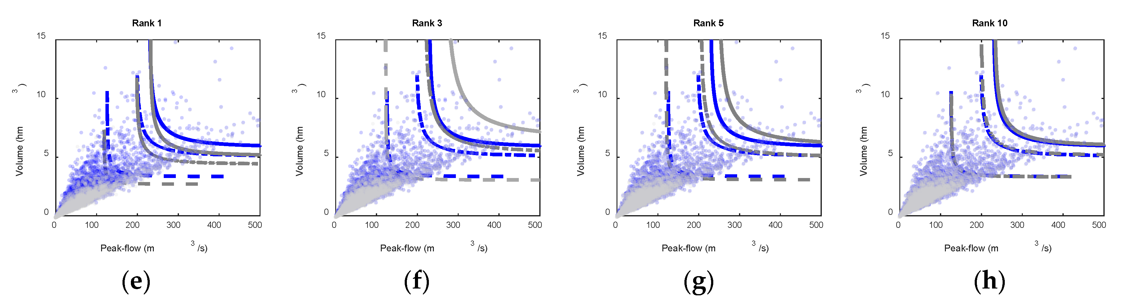
3.2.4. Magnitude and Recurrence. Copula-based Frequency Analysis

We fitted the three Archimedean copulas exposed in the methodology to the 5000 pairs of peak-flows and volumes using the MhAST Toolbox [46].

Table 6. Parameters of the Archimedean copula estimation from the pair of values of maximum annual peak-flows and maximum annual volumes of the continuous simulation, with the root mean square error (RMSE) and Nash–Sutcliffe error (NSE).

Copula	Parameter	RMSE	NSE
Clayton	3.10	1.68	0.992
Frank	11.5	0.58	0.999
Gumbel	2.98	0.70	0.998

shows the parameters estimated for each of the copulas, obtained by the method of maximum likelihood, with the value of RMSE and the NSE for each of the copula fits. For the studied copulas, the best fit corresponds to the Frank copula, followed closely by the Gumbel copula. As both Gumbel and Frank provided a good fit, we chose the Gumbel copula for further analysis as it is the only one of the three studied copulas able to model upper tail dependence [52].

Table 7. Parameters of the Gumbel copula estimation from the pair of values of maximum annual peak-flows and maximum annual volumes regarding the maximum storm rank considered and the criteria used: Total depth or maximum intensity, and relative error (RE) respect to the continuous simulation.

Maximum Storm Rank Considered	Total Depth		Maximum Intensity
	Gumbel Parameter	RE	Gumbel Parameter	RE
Continuous Simulation	2.98	−	2.98	−
Rank 1	2.94	1.37	4.84	−62.34
Rank 3	3.00	−0.79	3.82	−28.32
Rank 5	3.02	−1.18	3.40	−13.91
Rank 10	2.99	−0.25	3.08	−3.26

shows the parameter fit of the Gumbel copula for different storm ranks according to the two criteria studied. In the case of the V_Event criterion, the absolute RE is lower than 2% considering the storms up to any rank. Only in the case of considering storms up to rank ten with the total V_Event criterion, the absolute RE is lower than 0.5%. In the case of the I_max criterion, storm ranks up to ten should be considered for absolute values of RE lower than 5%. The results of Table 7 have a reflection when T_K are estimated. Figure 8 shows the T_K of 10 (dashed), 50 (dashed-dotted) and 100 (continuous) years of the continuous simulation (red (Figure 8a–d) and blue (Figure 8e–h) lines) compared to the different storm ranks according to V_Event and I_max criteria (grey lines in Figure 8).

According to each ranking criterion:

• V_Event. Visually, there is a good agreement between the T_K estimated with the V_Event criterion and the continuous simulation (Figure 8a–d). Worse agreement is shown for high return periods (100 years). In the case of considering storms with ranks up to ten (Figure 8d), the T_K are almost coincident.
• I_max. There is not a good agreement between the T_K estimated with this criterion compared to the continuous simulation for ranks up to three. If the biggest storm is considered, the T_Ks are underestimated. In the case of considering storm ranks up to three, the return periods of 50 and 100 years are highly overestimated. T_Ks are closer with storms up to rank five (still overestimated for 50 and 100 years T_Ks), and almost a perfect agreement is achieved if rank periods up to 10 are considered.

3.2.5. Discussion

As exposed, some studies in the literature have previously analyzed the influence of storms on the derivation of the flood frequency curve through event-based approaches.

Table 8. Comparison between similar case studies and the methodology used in each of them. For comparison purposes, the basin area, weather/rainfall generator, hydrological model and the way of accounting soil moisture are shown.

Case Study	Area (km2)	Weather/Rainfall Generator	Spatial Resolution	Hydrological Model	Type	Initial Soil Moisture
Peacheater Creek	64	AWE-GEN [28]	Punctual	TRIBS [6]	Fully distributed-Continuous	Continuous assessment
Générargues [23,53]	245	RainSim V3 [54]	Spatial-Punctual	RIBS [35]	Fully distributed-Event based	Probabilistic
Corbès [23,53]	262.3	RainSim V3 [54]	Spatial-Punctual	RIBS [35]	Semidistributed-Event based	Probabilistic
Navacerrada [55]	20	RainSim V3 [54]	Spatial-Punctual	Stochastic HEC-HMS [19,20]	Semidistributed-Event based	Deterministic
Santillana [27]	211	RainSim V3 [54]	Spatial-Punctual	Stochastic HEC-HMS [19,20]	Semidistributed-Event based	Deterministic
El Pardo [27]	495	RainSim V3 [54]	Spatial-Punctual	Stochastic HEC-HMS [19,20]	Semidistributed-Event based	Deterministic
Manzanares [27]	1294	RainSim V3 [54]	Spatial-Punctual	Stochastic HEC-HMS [19,20]	Semidistributed-Event based	Deterministic

shows the main characteristics of the research on this topic. Flores-Montoya et al. [23] (extended analysis in [53]) carried out a similar experiment in two French basins. They extracted the storms from the synthetic time series of spatial-punctual rainfall generated with the Rainsim V3 [54], and forced the event-based distributed model RIBS [35] (predecessor of tRIBS) with them. As they accounted for spatial variability, they separated the storms based on the mean area rainfall, and ranked them by total depth, mean intensity (instead of maximum intensity), and total duration. They carried out the analysis only for the five highest storms of each year, and performed the experiment simultaneously for Générarges and Corbès. Sordo-Ward et al. [27,55] performed a similar analysis in four Spanish basins, by also coupling the RainSim V3 with a simpler semi distributed model [19,20]. Thus, they were able to analyze all the events each year as the experiment resulted less computationally expensive.

When comparing to the present study, Sordo-Ward et al. [27,55] and Flores-Montoya et al. [23] both used event-based approaches instead of a continuous approach. As a consequence, they needed to characterize the soil-moisture in the basin prior to the storm events. In the case of Sordo-Ward et al. [27,55], they considered a constant value of the curve number in each of the sub-basins for all the storms. Regarding Flores-Montoya et al. [23], they determined the initial soil moisture in a probabilistic way. Within this study, as we performed the simulations with tRIBS, all the conditions prior to the storm events were given by the continuous simulation.

Table 9. Results obtained for the different case studies considered in Table 8. PF represents the maximum annual peak-flow, V represents the maximum annual volume, and RE represents the relative error.

Case Study	Best Criteria	1st Rank PF Coincidence (%)	1st rank V Coincidence (%)	Rank 95% PF	Rank 95% V	Rank Seasonality PF and V (<5% RE)	Rank Copula Parameter (<5% RE)
Peacheater Creek	Total depth	53	69	5	4	3	1
Générargues [23,53]	Total depth	70	88	4	2	−	−
Corbès [23,53]	Total depth	70	88	4	2	−	−
Santillana [27]	Total depth	66	−	4	−	−	−
El Pardo [27]	Total depth	67	−	4	−	−	−
Manzanares [27]	Total depth	55	−	6	−	−	−
Navacerrada [55]	Total depth	63	−	6	−	−	−

shows a summary of the results obtained within this paper and the comparison of the results obtained in other studies (some aspects have not been studied by the other compared studies and are therefore not shown). Several aspects can be remarked when analyzing Table 9:

• In all the case studies, among the three criteria of storm event ranking, the best was total depth. This suggests that the choice between one criterion or another has a low dependence on the hydrological model used or how the initial moisture is accounted. Accounting or not for the spatial variability of rainfall does not seem to influence either, but this might be due to the small size of Peacheater Creek.
• Regarding the probability of achieving the maximum annual peak-flow, the lowest values (55% and 53%) correspond to the Manzanares and Peacheater Creek, respectively. The first is the biggest basin (1294 km²), and the reduction of probability can be due to the importance of propagation processes and the temporal patterns of the storm events. However, Peacheater Creek is the second smallest basin in Table 9. The reduction of the coincidence with the maximum annual peak-flow might be due to how antecedent basin conditions prior to the storm event are considered. As the model is continuous, some lower rank events may concur with wetness states of the basin, incurring higher peak-flows. This phenomenon cannot occur in the Sordo-Ward et al. [27,55] study basins, as the initial soil moisture was considered constant and equal for all the storm events.
• When the coincidence of the first rank total depth storm with the maximum annual volume is analyzed (Peacheater Creek and Flores-Montoya et al. [23]), we can see that there is a higher probability of coincidence than that of the peak-flow. This suggests that total depth has a better correlation with the maximum annual volume than with the maximum annual peak-flow. This can also be seen when the minimum rank of storm required is analyzed. Smaller ranks are required to achieve a 95% probability of obtaining the maximum annual volume than for obtaining the maximum annual peak-flow with the same probability.
• In all the case studies shown, the maximum peak-flow can be obtained with a 95% probability considering all the storms up to rank four, five or six. In the case of total volume, the maximum rank required is reduced to two or four.
• Within this manuscript, we have shown that seasonality and bivariate properties of extreme floods can be well-preserved if storms up to rank three and one are considered, respectively.

Therefore, to sum up, as a general recommendation, considering the five biggest storms per year classified by their total depth can result in an accurate derivation of the flood frequency curve when using event-based models, close to that obtained from continuous simulations. Future works can be focused on analyzing different case studies with different rainfall–runoff models.

4. Summary and Conclusions

This paper approaches a focus on providing guidance on selecting the minimum number of storm events for deriving the flood frequency curve through event-based approaches. To do so, the methodology applied compares the resulting flow of coupling a stochastic weather generator with a fully distributed physically-based model with the flow resulting from selecting only a limited number of storms per year. The methodology has only been applied to one basin, and therefore the results and conclusions are restricted to this watershed. Despite this, the study shows how the number of storms selected has an influence on the derivation of extreme floods, and its characteristics: Univariate magnitude and recurrence of maximum annual peak-flows and volumes, their seasonality, their dependence, and their statistic bivariate properties. Specifically, for Peacheater Creek:

• When analyzing the correspondence between storms and maximum annual peak-flow and volume, the best ranking criterion is total depth, followed by maximum intensity. Considering storms up to rank five sorted by the total depth criterion, resulted in a probability of generating the maximum annual peak-flow of 94% and the maximum annual volume of 99%.
• In the case of the total depth criterion, the higher the return period of peak-flow or volume is, the lower the storm rank needed. For return periods of peak-flow or volume over ten years, all the storms have a rank equal or lower than four. For return periods higher than 50 years, there is a probability of achieving the maximum annual peak-flow and the maximum annual volume of 99% if the three highest events are considered.
• For preserving the seasonality of maximum annual peak-flows and volumes, total depth was also the best criterion. With storms up to rank five, there is less than 1% absolute relative error in the estimation of the mean direction of seasonality for both the peak-flow and volume. Regarding the dispersion of the seasonality, considering storms up to rank five resulted in an absolute relative value lower than 4%.
• Total depth was also the best criterion for preserving the dependence and bivariate properties of the floods derived from the continuous simulation. Even by considering only the biggest storm of each year, the absolute relative errors when estimating Spearman’s rho and Kendall’s tau are less than 1%. When estimating the parameter of the copula family selected (Gumbel), the relative error was less than 2% if storms up to any rank were considered, and was less than 0.5% if storms up to rank ten were considered. Regarding Kendall’s return period, considering the same number of storms produces Kendall’s return periods of 10 and 50 years very similar to those obtained by continuous simulation, and the 100 years return period is slightly underestimated. If the ten biggest storms are considered, all the studied Kendall’s return periods are almost equal.

References

1. Fatichi, S.; Vivoni, E.R.; Ogden, F.L.; Ivanov, V.Y.; Mirus, B.; Gochis, D.; Downer, C.W.; Camporese, M.; Davison, J.H.; Ebel, B.; et al. An overview of current applications, challenges, and future trends in distributed process-based models in hydrology. J. Hydrol. 2016, 537, 45–60. [Google Scholar] [CrossRef] [Green Version]
2. Blazkova, S.; Beven, K. Flood frequency estimation by continuous simulation of subcatchment rainfalls and discharges with the aim of improving dam safety assessment in a large basin in the Czech Republic. J. Hydrol. 2004, 292, 153–172. [Google Scholar] [CrossRef]
3. Cui, Z.; Vieux, B.E.; Neeman, H.; Moreda, F. Parallelisation of a distributed hydrologic model. Int. J. Comput. Appl. Technol. 2005, 22, 42–52. [Google Scholar] [CrossRef]
4. Kollet, S.J.; Maxwell, R.M.; Woodward, C.S.; Smith, S.; Vanderborght, J.; Vereecken, H.; Simmer, C. Proof of concept of regional scale hydrologic simulations at hydrologic resolutions utilizing massively parallel computing resources. Water Resour. Res. 2010, 46, W0421. [Google Scholar] [CrossRef]
5. Vivoni, E.R.; Mascaro, G.; Mniszewski, S.; Fasel, P.; Springer, E.P.; Ivanov, V.Y.; Bras, R.L. Real-world hydrologic assessment of a fully-distributed hydrological model in a parallel computing environment. J. Hydrol. 2011, 409, 483–496. [Google Scholar] [CrossRef]
6. Pumo, D.; Arnone, E.; Francipane, A.; Caracciolo, D.; Noto, L.V. Potential implications of climate change and urbanization on watershed hydrology. J. Hydrol. 2017, 554, 80–99. [Google Scholar] [CrossRef]
7. Arnone, E.; Pumo, D.; Francipane, A.; La Loggia, G.; Noto, L.V. The role of urban growth, climate change, and their interplay in altering runoff extremes. Hydrol. Process. 2018, 32, 1755–1770. [Google Scholar] [CrossRef]
8. Liuzzo, L.; Noto, L.V.; Vivoni, E.R.; La Loggia, G. Basin-scale water resources assessment in Oklahoma under synthetic climate change scenarios using a fully distributed hydrological model. J. Hydrol. Eng. 2010, 15, 107–122. [Google Scholar] [CrossRef]
9. Piras, M.; Mascaro, G.; Deidda, R.; Vivoni, E.R. Quantification of hydrologic impacts of climate change in a Mediterranean basin in Sardinia, Italy, through highresolution simulations. Hydrol. Earth Syst. Sci. 2014, 18, 5201–5217. [Google Scholar] [CrossRef]
10. Ren, M.; He, X.; Kan, G.; Wang, F.; Zhang, H.; Li, H.; Cao, D.; Wang, H.; Sun, D.; Jiang, X.; et al. A Comparison of Flood Control Standards for Reservoir Engineering for Different Countries. Water 2017, 9, 152. [Google Scholar] [CrossRef]
11. Zhang, L.; Singh, V.P. Trivariate flood frequency analysis using the Gumbel–Hougaard copula. J. Hydrol. Eng. 2017, 12, 431–439. [Google Scholar] [CrossRef]
12. Klein, B.; Pahlow, M.; Hundecha, Y.; Schumann, A. Probability analysis of hydrological loads for the design of flood control systems using copulas. J. Hydrol. Eng. 2010, 15, 360–369. [Google Scholar] [CrossRef]
13. Katz, R.W.; Parlange, M.B.; Naveau, P. Statistics of extremes in hydrology. Adv. Water Resour. 2002, 25, 1287–1304. [Google Scholar] [CrossRef] [Green Version]
14. Salinas, J.L.; Laaha, G.; Rogger, M.; Parajka, J.; Viglione, A.; Sivapalan, M.; Blöschl, G. Comparative assessment of predictions in ungauged basins – Part 2: Flood and low flow studies. Hydrol. Earth Syst. Sci. 2013, 17, 2637–2652. [Google Scholar] [CrossRef]
15. Li, J.; Thyer, M.; Lambert, M.; Kuczera, G.; Metcalfe, A. An efficient causative event-based approach for deriving the annual flood frequency distribution. J. Hydrol. 2014, 510, 412–423. [Google Scholar] [CrossRef] [Green Version]
16. Adams, B.; Howard, C.D. Design storm pathology. Can. Water Resour. J. 1986, 11, 49–55. [Google Scholar] [CrossRef]
17. Alfieri, L.; Laio, F.; Claps, P. A simulation experiment for optimal design hyetograph selection. Hydrol. Process. 2008, 22, 813–820. [Google Scholar] [CrossRef]
18. Viglione, A.; Blöschl, G. On the role of storm duration in the mapping of rainfall to flood return periods. Hydrol. Earth Syst. Sci. 2009, 13, 205–216. [Google Scholar] [CrossRef] [Green Version]
19. Sordo-Ward, A.; Garrote, L.; Martin-Carrasco, F.; Bejarano, M.D. Extreme flood abatement in large dams with fixed-crest spillways. J. Hydrol. 2012, 466, 60–72. [Google Scholar] [CrossRef]
20. Sordo-Ward, A.; Garrote, L.; Bejarano, M.D.; Castillo, L.G. Extreme flood abatement in large dams with gate-controlled spillways. J. Hydrol. 2013, 498, 113–123. [Google Scholar] [CrossRef]
21. Foufoula-Georgiou, E. A probabilistic storm transposition approach for estimating exceedance probabilities of extreme precipitation depths. Water Resour. Res. 1989, 25, 799–815. [Google Scholar] [CrossRef]
22. Franchini, M.; Helmlinger, K.R.; Foufoula-Georgiou, E.; Todini, E. Stochastic storm transposition coupled with rainfall-runoff modeling for estimation of exceedance probabilities of design floods. J. Hydrol. 1996, 175, 511–532. [Google Scholar] [CrossRef]
23. Flores-Montoya, I.; Sordo-Ward, Á.; Mediero, L.; Garrote, L. Fully Stochastic Distributed Methodology for Multivariate Flood Frequency Analysis. Water 2016, 8, 225. [Google Scholar] [CrossRef]
24. Haberlandt, U.; Ebner von Eschenbach, A.D.; Buchwald, I. A space-time hybrid hourly rainfall model for derived flood frequency analysis. Hydrol. Earth Syst. Sci. 2008, 12, 1353–1367. [Google Scholar] [CrossRef] [Green Version]
25. Brocca, L.; Liersch, S.; Melone, F.; Moramarco, T.; Volk, M. Application of a model-based rainfall-runoff database as efficient tool for flood risk management. Hydrol. Earth Syst. Sci. 2013, 17, 3159–3169. [Google Scholar] [CrossRef] [Green Version]
26. Paquet, E.; Garavaglia, F.; Garçon, R.; Gailhard, J. The SCHADEX method: A semi-continuous rainfall–runoff simulation for extreme flood estimation. J. Hydrol. 2013, 495, 23–37. [Google Scholar] [CrossRef]
27. Sordo-Ward, A.; Bianucci, P.; Garrote, L.; Granados, A. The Influence of the Annual Number of Storms on the Derivation of the Flood Frequency Curve through Event-Based Simulation. Water 2016, 8, 335. [Google Scholar] [CrossRef]
28. Fatichi, S.; Ivanov, V.Y.; Caporali, E. Simulation of future climate scenarios with a weather generator. Adv. Water Resour. 2011, 34, 448–467. [Google Scholar] [CrossRef]
29. Ivanov, V.Y.; Vivoni, E.R.; Bras, R.L.; Entekhabi, D. Catchment hydrologic response with a fully distributed triangulated irregular network model. Water Resour. Res. 2004, 40, W11102. [Google Scholar] [CrossRef]
30. Vivoni, E.R.; Entekhabi, D.; Bras, R.L.; Ivanov, V.Y. Controls on runoff generation and scale-dependence in a distributed hydrologic model. Hydrol. Earth Syst. Sci. 2007, 11, 1683–1701. [Google Scholar] [CrossRef] [Green Version]
31. Restrepo-Posada, P.J.; Eagleson, P.S. Identification of independent rainstorms. J. Hydrol. 1982, 55, 303–319. [Google Scholar] [CrossRef]
32. Ivanov, V.Y.; Bras, R.L.; Curtis, D.C. A weather generator for hydrological, ecological, and agricultural applications. Water Resour. Res. 2007, 43, 40. [Google Scholar] [CrossRef]
33. Cowpertwait, P.S.P. Mixed rectangular pulses models of rainfall. Hydrol. Earth Syst. Sci. 2004, 8, 993–1000. [Google Scholar] [CrossRef] [Green Version]
34. Nelder, J.; Mead, R. A simplex method for function minimization. Comput. J. 1965, 7, 308–313. [Google Scholar] [CrossRef]
35. Garrote, L.; Brass, R.L. An integrated software environment for real-time use of a distributed hydrologic model. J. Hydrol. 1995, 167, 307–326. [Google Scholar] [CrossRef] [Green Version]
36. Vivoni, E.R.; Ivanov, V.Y.; Bras, R.L.; Entekhabi, D. Generation of triangulated irregular networks based on hydrologic similarity. J. Hydrol. Eng. 2004, 9, 288–302. [Google Scholar] [CrossRef]
37. Sifalda, V. Entwicklung eines Berechnungsregens für die Bemessung von Kanalnetzen. Wasser Abwasser 1963, 114, 435–440. [Google Scholar]
38. Yen, B.C.; Chow, V.T. Design hyetographs for small drainage structures. J. Hydraul. Div. 1980, 106, 1055–1076. [Google Scholar]
39. Bonta, J.V.; Rao, A.R. Factors affecting the identification of independent storm events. J. Hydrol. 1988, 98, 275–293. [Google Scholar] [CrossRef]
40. Gringorten, I.I. A plotting rule for extreme probability paper. J. Geophys. Res. 1963, 68, 813–814. [Google Scholar] [CrossRef]
41. Berens, P. CircStat: A MATLAB Toolbox for Circular Statistics. J. Stat. Softw. 2009, 31, 1–21. [Google Scholar] [CrossRef]
42. Parajka, J.; Kohnová, S.; Bálint, G.; Barbuc, M.; Borga, M.; Claps, P.; Cheval, S.; Dumitrescu, A.; Gaume, E.; Hlavcová, K.; et al. Seasonal characteristics of flood regimes across the Alpine–Carpathian range. J. Hydrol. 2010, 394, 78–89. [Google Scholar] [CrossRef] [PubMed]
43. Fisher, N.I.; Switzer, P. Chi-Plots for Assessing Dependence. Biometrika 1985, 72, 253–265. [Google Scholar] [CrossRef]
44. Fisher, N.I.; Switzer, P. Graphical assessment of dependence: Is a picture worth 100 tests? Am. Stat. 2001, 55, 233–239. [Google Scholar] [CrossRef]
45. Genest, C.; Favre, A.C. Everything you always wanted to know about copula modeling but were afraid to ask. J. Hydrol. Eng. 2007, 12, 347–368. [Google Scholar] [CrossRef]
46. Sadegh, M.; Moftakhari, H.M.; Gupta, H.V.; Ragno, E.; Mazdiyasni, O.; Sanders, B.F.; Matthew, R.A.; AghaKouchak, A. Multi-Hazard Scenarios for Analysis of Compound Extreme Events. Geophys. Res. Lett. 2018, 45, 5470–5480. [Google Scholar] [CrossRef]
47. Salvadori, G.; De Michele, C. Multivariate multiparameter extreme value models and return periods: A copula approach. Water Resour. Res. 2010, 46, W10501. [Google Scholar] [CrossRef]
48. Brunner, M.I.; Seibert, J.; Favre, A.C. Bivariate return periods and their importance for flood peak and volume estimation. Wiley Interdiscip. Rev. Water 2016, 3, 819–833. [Google Scholar] [CrossRef] [Green Version]
49. Ivanov, V.Y.; Vivoni, E.R.; Bras, R.L.; Entekhabi, D. Preserving high-resolution surface and rainfall data in operational-scale basin hydrology: A fully-distributed physically-based approach. J. Hydrol. 2004, 298, 80–111. [Google Scholar] [CrossRef]
50. Sirisena, T.A.J.G.; Maskey, S.; Ranasinghe, R.; Babel, M.S. Effects of different precipitation inputs on streamflow simulation inthe Irrawaddy River Basin, Myanmar. J. Hydrol. Reg. Stud. 2018, 19, 265–278. [Google Scholar] [CrossRef]
51. Karypis, G.; Kumar, V. A fast and high quality multilevel scheme for partitioning irregular graphs. SIAM J. Sci. Comput. 1999, 20, 359–392. [Google Scholar] [CrossRef]
52. Poulin, A.; Huard, D.; Favre, A.C.; Pugin, S. Importance of Tail Dependence in Bivariate Frequency Analisys. J. Hydrol. Eng. 2007, 12, 394–403. [Google Scholar] [CrossRef]
53. Flores-Montoya, I. Generación de Hidrogramas de Crecida Mediante Simulación Estocástica Multivariada de Lluvia y Modelación Hidrológica Distribuida: Aplicación a Seguridad de Presas. Ph.D. Thesis, Technical University of Madrid, Madrid, Spain, 2018. (In Spanish). [Google Scholar] [CrossRef]
54. Burton, A.; Kilsby, C.G.; Fowler, H.J.; Cowpertwait, P.S.P.; O’Connell, P.E. RainSim: A spatial–temporal stochastic rainfall modelling system. Environ. Model. Softw. 2008, 23, 1356–1369. [Google Scholar] [CrossRef]
55. Sordo-Ward, A.; Bianucci, P.; Garrote, L. Influencia del número de tormentas consideradas por año para la generación de la ley de frecuencia de caudales. In Proceedings of the 4th Jornadas de Ingeniería del Agua: La Precipitación y Los Procesos Erosivos, Cordoba, Spain, 21–22 October 2015. (In Spanish). [Google Scholar]
Figure 1. General scheme of the methodological approach.
Water 11 01896 g001
Figure 2. Example of two independent rainfall events (black and grey for events one and two, respectively). The total depth of the event (VEvent) is represented by the shaded area, the maximum intensity (Imax) is represented by the dots, and the duration (DEvent) by the lower line. Two dry periods are represented in the figure. The first one, has a shorter duration than the minimum inter-event time (MIT) and therefore, the two wet periods belong to the same event. In the second dry period, the duration is longer than the MIT and it represents the separation between the two events.
Water 11 01896 g002
Figure 3. Case study and model setup. (a) Basin location, elevation, and drainage network. (b) Discretization of the basin into Voronoi polygons for triangulated irregular network real-time integrated basin simulator (tRIBS). (c) Partitioning of the basin for parallel computation using eight processors.
Water 11 01896 g003
Figure 4. Validation of the generated rainfall series. (ad) Comparison between the observed rainfall frequency curve (blue dots) (obtained by applying the Gringorten plotting position formula [40]) and synthetic rainfall frequency curves obtained by bootstrapping 1000 series of 40 years of hourly rainfall obtained from the 5000 years of synthetic weather series generated: (a) Maximum annual cumulated rainfall (P) in: (a) 1 h, (b) 6 h, (c) 12 h, and (d) 24 h. (e) Comparison between the seasonality of the observed maximum annual intensity (blue circles), with the predominant direction (blue line) compared to the predominant direction of the seasonality of 1000 series of 20 years of maximum annual depth obtained by bootstrapping from the 5000 years of synthetic weather generated (in grey lines), with the mean predominant direction represented in black. (f) The same as e, but for total depth, with observed values represented in red circles.
Water 11 01896 g004aWater 11 01896 g004b
Figure 5. Storm order that corresponds to every return period (Tr) of maximum annual peak-flow (a) and maximum annual volume (b) represented as red dots for the total depth criteria and as blue dots for the maximum intensity rank criteria. The numbers on the right represent the probability that a storm of a specific rank generates the maximum peak-flow (a) or volume (b) of given a yea.
Water 11 01896 g005
Figure 6. Comparison between the seasonality of the observed maximum annual peak-flow (red lines in (a–d); and blue lines in (il) and maximum annual volume (red lines eh; and blue lines (mp) with respect to that obtained by applying different criteria (total depth (ah) and maximum intensity (ip)) and accounting for different rank orders (up to one, three, five and ten), in which the predominant direction of the seasonality is represented by a circle with a black line.
Water 11 01896 g006
Figure 7. Chi-plots of the maximum annual peak-flow and volume. Grey dots represent the values obtained considering specific storm orders up to different ranks (a,e) rank one (b,f) rank three, (c,g) rank five, (d,h) rank ten). Color dots represent the values obtained from the continuous simulation (red in (ad), blue (eh)). Storm rank criteria are total depth in (ad) and maximum intensity in (eh).
Water 11 01896 g007aWater 11 01896 g007b
Figure 8. Chi-plots of maximum annual peak-flow and volume. Grey dots represent the values obtained considering specific storm orders up to different ranks (a,e) rank one (b,f) rank three, (c,g) rank five, (d,h) rank ten). Color dots represent the values obtained from the continuous simulation (red in (ad), blue (eh)). Storm rank criteria is total depth in (a–d) and maximum intensity in (eh).
Water 11 01896 g008aWater 11 01896 g008b