High Resolution Monitoring of Seawater Intrusion in a Multi-Aquifer System-Implementation of a New Downhole Geophysical Tool

Abstract

Monitoring of seawater intrusion is extremely important for the management of coastal aquifers, and therefore requires reliable and high-frequency monitoring tools. This paper describes the use of a new near field and downhole geophysical tool that monitors seawater intrusion in boreholes with high vertical resolution. This sensor is further used to study the impact of pumping on water electrical conductivity profiles (ECP) at the fresh-saline water interface. The new device was installed in a confined calcareous sandstone aquifer along the northern Israeli coast. The site includes two monitoring wells and one pumping well located at distances of 50, 75 and 125 m from shoreline, respectively. The new geophysical tool, called the subsurface monitoring device (SMD), was examined and compared to water an electric conductivity profiler (ECP) and a conductivity temperature depth (CTD) driver’s data. All methods show similar salinity trends, and changes in pumping regime were clearly identified with both the SMD and CTD. The advantage of using the SMD tool is the high temporal and spatial resolution measurement, which is transferred via internet and can be analyzed and interpreted in real time. Another advantage of the SMD is that it measures the electrical resistivity of the aquifer mostly outside the well, while both water ECP and the CTD measure in-well electrical conductivity; therefore, are subjected to the artefact of vertical flow in the well. Accordingly, while the CTD shows an immediate and sharp response when pumping is stopped, the SMD provides a gradual electric conductivity (EC) change, demonstrating that stability is reached just after a few days, which illustrates, more precisely, the hydrological response of the aquifer.

1. Introduction

Seawater intrusion (SWI) is of global concern, exacerbated by increasing demands for freshwater in coastal zones and predisposed to the influences of rising sea levels and changing climates. The extent and the dynamics of seawater intrusion into coastal aquifers is commonly estimated by the rise in salinity in monitoring wells or deduced from hydrological models (e.g., [1]). The SWI monitoring network includes measurements of water electric conductivity (EC) profiles that record the location of the fresh-saline water interface (FSI), using manual logging probes [1]. Since the early 1980s, many articles have discussed distorted observations obtained in long-perforated observation boreholes due to the effect of vertical flow [2,3,4,5]. It has been further shown by 3D numerical modelling that vertical flow in a borehole can cause water EC fluctuations that are one order of magnitude larger than the original seawater tidal fluctuation [6]. This was confirmed by [7], using buried EC sensors, which further suggested that monitoring of the transition zone between fresh and saline water adjacent to the sea through long-perforated boreholes is unreliable. The mentioned bias between borehole measurements and actual aquifer FSI fluctuations could be overcome by in situ geophysical methods, which measure resistivity in the aquifer outside the borehole.

The large electrical resistivity contrast between seawater (0.2 Ωm) and freshwater (>5 Ωm) makes it possible to map the subsurface groundwater salinity distribution using geophysical techniques (e.g., [8,9]). Direct current (DC)-resistivity, electromagnetic (EM) methods in particular, have been applied successfully in coastal areas [10]. The recent development of the EM method of multi-electrode resistivity array, which is permanently installed in the well, allows mapping of the subsurface salinity distribution in unprecedented time resolution, and a detailed documentation of the temporal dynamics of salinity distribution in the aquifer [11,12]. This tool can reduce existing gaps in the understanding of SWI timeframes, and will allow the characterization and prediction of FSIs in highly heterogeneous and dynamic coastal settings. In small scale inhomogeneity, the use of downhole geophysical tool is more complicated because the conversion of resistivity into water EC needs to consider the difference in soil resistivity. Another difficulty is the costs, which are generally higher than the common methods for the electric conductivity profiler (RG, WTW).

The objective of this research was to examine the new multi-electrode-resistivity tool, the s (SMD), for monitoring seawater intrusion in high time resolution. Compared to cross-hole electrical resistivity, a single well is needed for SMD measurement. It measures bulk resistivity around the well with a better resolution, and a direct conversion allows Water Electric Conductivity (ECw) determination. This method is cheaper than cross-hole electrical resistivity, although cross-hole electrical resistivity allows a larger measurement area between the wells. We show below that the SMD is highly efficient in monitoring the changes in the fresh-saline water interface due to local and regional water withdrawal. Another successful application of the SMD monitoring device was conducted in Deltares, Nethrlands. The SMD was used there to monitor the fresh water lenses’ development during the reinjection process of fresh water within a saline aquifer to increase fresh water lenses below agricultural area aquifer.

2. Hydrogeological Background of the Study Area

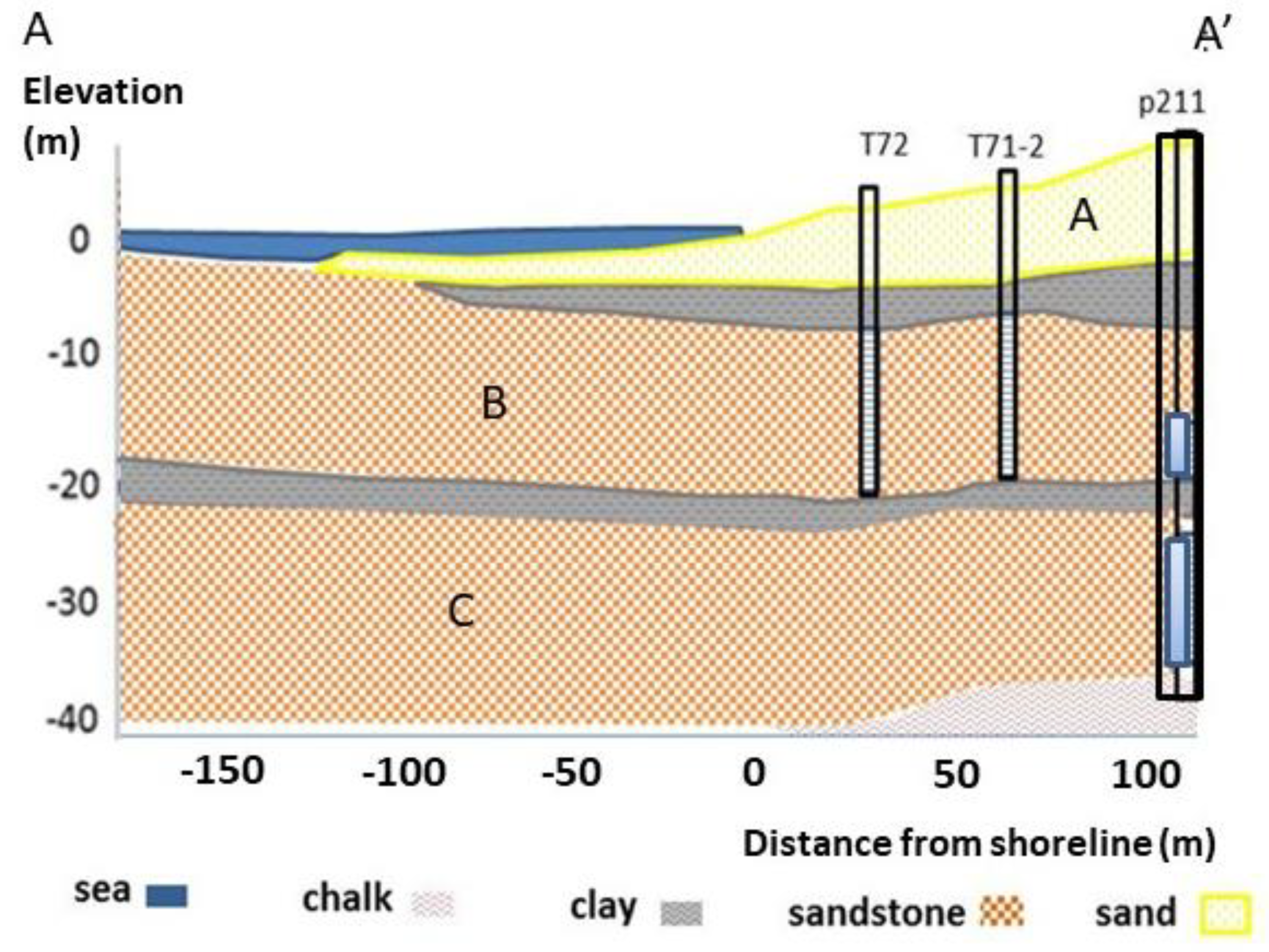
The study area is located at the southern part of the Mt. Carmel coastal plain, in the Maagan Michael area, adjacent to the Mediterranean Sea (Figure 1). The width of the coastal aquifer from the sea to Mt. Carmel is 5 km. It consists of Pleistocene to Holocene sediments with a thickness of about 40 m, which are underlain by Late Cretaceous carbonates [13]. The aquifer includes three sub-aquifers (Figure 2). The upper sub-aquifer is a phreatic Holocene sandy unit (unit A) with a thickness of several meters, which is separated from the underlying Pleistocene calcareous sandstone (locally called Kurkar) aquifer by a clay unit. The Pleistocene Kurkar is subdivided by another clay layer into two confined units, B and C, which are underlain by Late Cretaceous chalk aquitard [14]. This chalks’ change eastward to the dolomite facies of the Late Cretaceous Yarkon Taninim aquifer [15,16,17]. The main water source for the coastal Pleistocene confined units in this area is the Yarkon Taninim aquifer, while the current recharge to the sandy phreatic unit is mainly through losses from fishponds that cover the study area [14]. The Pleistocene aquifer, which contains brackish water (1500–2000 mg/L Cl), was extensively exploited since 2005 for the fish ponds and for a local desalination plant, with pumping currently reaching ~20 × 10⁶ m³ yr⁻¹. Although exploitation is very high, the water level in this area is quite stable, and seawater intrusion is limited. This is explained by the increase of inflow from the underlying Yarkon Taninim aquifer [18]. Offshore geophysical surveys by CHIRP (Compressed High Intensity Radar Pulse) in the shallow sea showed that the offshore extension of the shallow clay layer, which confines unit B, reaches more than 700 m in the northern part of the study area, while at the southern part of the area is missing already, at 100 m offshore. The CHIRP results indicate that seawater intrusion can take place, as observed in unit B (not in the underlying unit C and the overlaying unit A) at the southern part 75 m from sea, and not at the northern part. This was supported by numerical simulations, which showed that the difference in the offshore extension of the clay may delay SWI by years [18]. The hydraulic conductivity determined by field tests for units A, B and C were 30, 68 and 109 m/day, respectively, and the storativity in units B and C were 0.0001 and 0.0016, respectively [18]. The porosity ranges of the Kurkar in this area is 0.15–0.25. The depth of the fresh/salt water interface in Unit B at well T71-2 was ~22 m (−19 masl) and in well T72, ~21.5 m (−20.5 masl).

3. Methodology

The current study was conducted in the southern part of the area where SWI was observed. The study area includes two observation wells screened at unit B (T72 and T71-2), located 50 and 75 m from shore, respectively, and one pumping well (P211) opened both to unit B and to unit C, which is located 125 m from the sea (Figure 2). Due to pumping, water level in unit B (which is the subject of this study) is on the average 1.1 and 1.3 m lower than in the overlaying unit A and the underlying unit C, respectively [18]. Profiles in units A and C, 75 m from shore, show low and uniform EC values (5–6 mS/cm, like the natural conductivity in this area), while in unit B an interface was observed at a depth of 22 m, and salinity of bottom water reached 40 mS/cm [18]. In this study, electrical conductivity was measured by several methods:

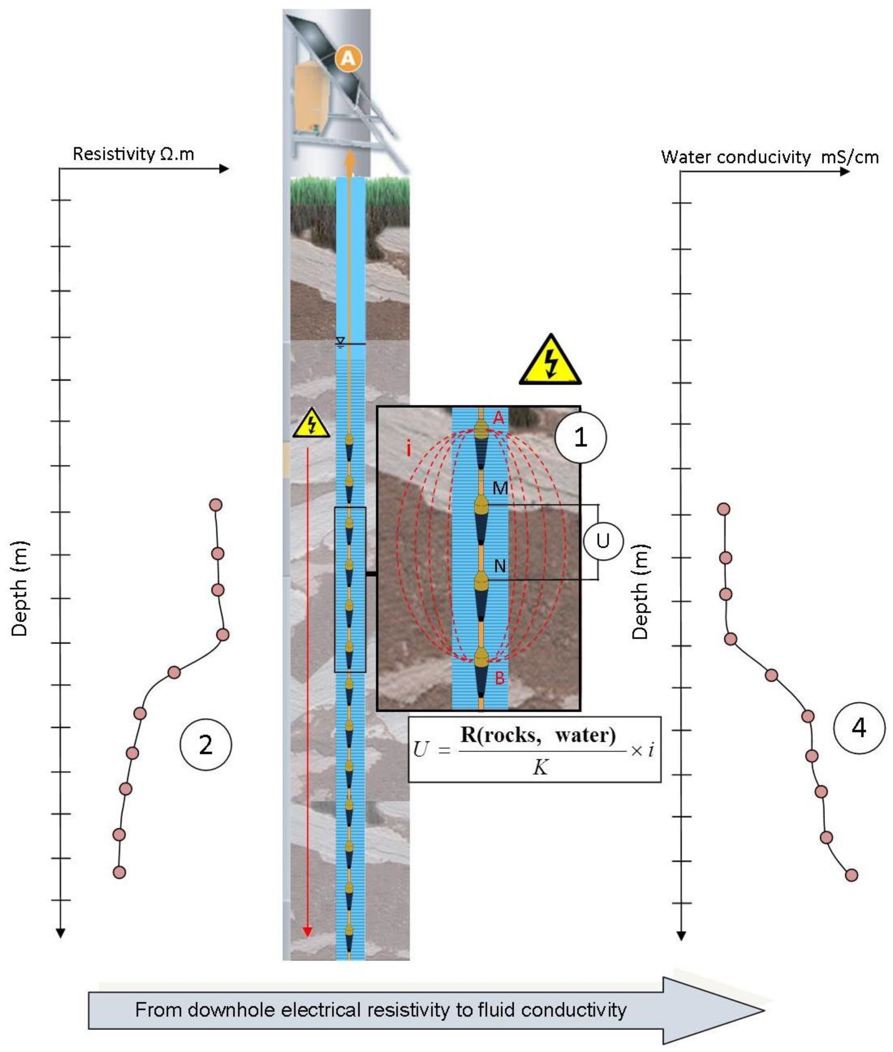
SMD (subsurface monitoring device) is a new automatic, remote-controlled multi sensor geophysical tool, which allows the measurement of water EC profiles and other parameters, such as water level and temperature profiles [19,20,21,22,23]. The SMD includes a cable loaded with electrodes which is deployed in a borehole and provides a profile of the resistivity of the rock formation around the borehole. A surface data acquisition box injects a known current between electrodes and measures the induced potential difference between two other electrodes (Figure 3). Bulk resistivity is obtained using Ohm’s law, corrected by a geometric factor. This process is repeated from the top to the bottom of the electrode cable, allowing the measurement of bulk resistivity profiles. Bulk resistivity, which is affected by the water salinity, porosity and rock type, is converted into EC of the liquid, using the Waxman–Smits equation. This conversion considers the formation factor (F), and the surface conductivity term (Cs), which are determined using a reduced set of logging measurements (gamma ray, resistivity and sonic for porosity).

Waxman–Smits equation:

$$Cw=\left(\frac{1}{Ro}-Cs\right)F$$

where

• C_w—water conductivity;
• Ro—measured resistivity;
• Cs—surface conductivity due to clay. Linear function of the natural gamma radioactivity (GR);
• F = formation factor. This factor depends on matrix porosity and pore connectivity index and is given by Archie’s law $F={\Phi }^{-m}$, where Ø = porosity and m = cementation index. The porosity can usually be measured on core, in laboratory. The Cementation index (m) can vary from 1.3 for non-consolidated sands to 2.5 for cemented carbonates.

The electrodes are made of a cupro-aluminum allowing reduction of the corrosion process. The energizing power was 12 V (battery or solar type), with the possibility of being plugged to the mains. The current intensity injected: Low power is 0.5 A, high power is 2 A. The equipment can be installed down to 200 m depth downhole, with up to 250 electrodes. Range of resistivity measurement: From 0.5 Ω. m to 5000 Ω. m. Lifespan: Over 8 years (several thousand measurements).

The data is transferred by telecommunication and may be visible on an internet interface. The radial resolution in the SMD is 40% to 50% of the spacing between electrodes, namely: For 1 m spacing, the radial resolution is 40–50 cm. 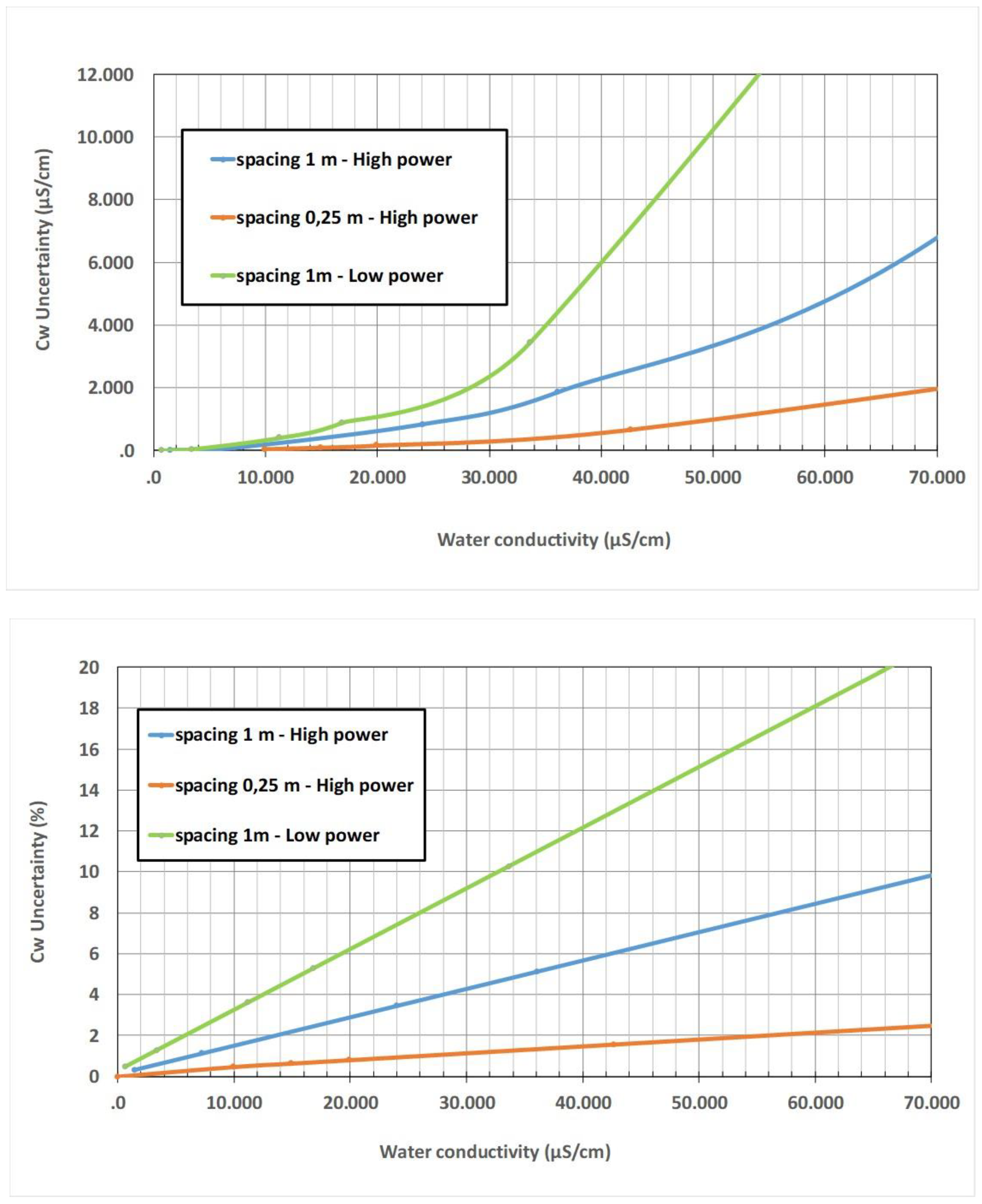Accordingly, the measured resistivity mostly represents salinity of groundwater outside the well, whose diameter is 2” (about 5 cm) and has a 5.5” drilling diameter, thus, avoiding the well vertical flow effect [7]. With shorter spacing between electrodes, the measured resistivity has shorter radial resolution, and accordingly may be more affected by the well. The specific conditions of SMD measurements can be controlled remotely; i.e., time and space resolution can be changed without a visit to the field. The SMD tool has been specifically developed for FSI monitoring, and accordingly it measures conductivities between 2–40 mS/cm (which is about 5–75% of seawater conductivity). The accuracy depends on the injection power, electrode spacing and water salinity. It improves when injection power is high and electrode spacing and water salinity is low (Figure 4). In very salty water (sea water), the accuracy of the SMD decreases.

The SMD system was installed in June 2014 in well 71-2 (Figure 1 and Figure 2), which is 24 m deep. The system included an array of 19 electrodes, separated by 1 m between 13–21 m from the borehole head and by 0.25 m between 21–23.5 m. While for a 1 m spacing the radial resolution is ~50 cm, for the 25 cm spacing it is ~13 cm (borehole casing diameter is 2”; i.e., radius of ~2.5 cm). Pressure sensor was installed at 8 m depth, in order to monitor the groundwater level. In order to have a continuous measurement of the EC, a daily frequency measurement was set.

Electrical conductivity profiles (ECP) were taken manually twice a year during 2014–2016, using a Robertson Geologging (RG) profiler. The compensated electrical conductivity profile was used.

CTD divers (Schlumberger) were deployed in well 71-2 and in 72 (Figure 2), and measured EC with 1-h frequency. The divers were deployed at a depth of 22 m, which was changed in well 71-2 to 20.5 m after the installation of the SMD. The SMD time resolution was changed to 1-h frequency, and that of the CTD diver was changed to 0.5-h frequency for a short period of about 48 h during 29 September–1 October 2014, in order to examine the effect of pumping on borehole salinity.

Operational Aspects of the SMD Method

While the raw data obtained with CTD and ECP can be directly converted to water salinity, SMD interpretation is more complex due to the dependence of the resistivity-salinity conversion on aquifer rock parameters. Nevertheless, since rock resistivity doesn’t change with time, changes in resistivity could be directly attributed to changes in water salinity; therefore, shortening the interpretation process.

The remote transmission of the SMD method is a big advantage over the EC profiler. The power supply for the SMD in this study included two batteries (12 volts; 100 A h) for safety reasons, since the solar panel was sensitive to vandalism. Except for the replacement of batteries at a frequency of about one month, no special maintenance was required. The main difficulty was the weight of the batteries (about 35 kg per battery), which makes their replacement difficult, requiring access for a vehicle. This problem was solved in the latter part of the research, when solar energy was used, secured against vandalism. The SMD user interface allows easy and friendly access to the data and displays results in different graphical formats, including the export of data to Excel. The specific conditions of SMD measurements can be controlled remotely; i.e., time and space resolution can be changed without a visit to the field. This could be very important for cases where the research is conducted in very remote areas.

4. Results and Discussions

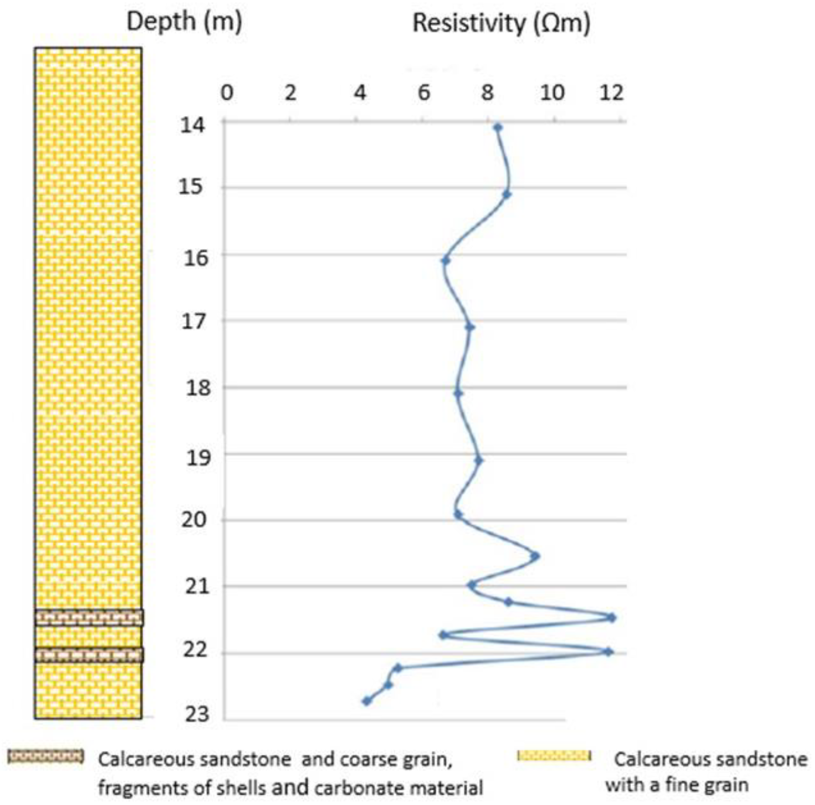
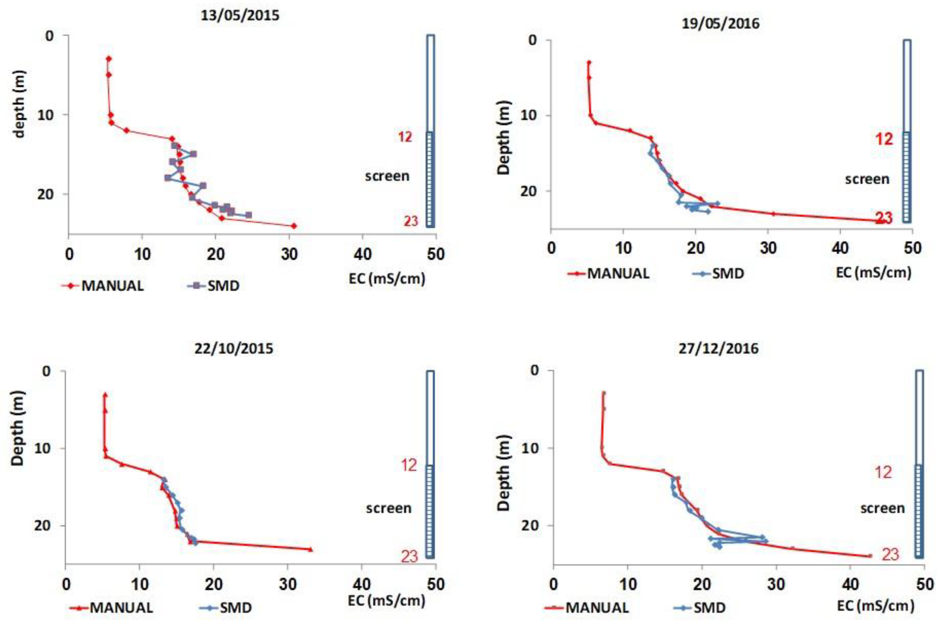
This chapter deals with the results of the new SMD method and compares them with the other, more conventional EC methods. Figure 5 shows the Electrical resistivity profile and a schematic log in well 71-2. The most coarse-grained zone is indicated with relatively high resistivity. Figure 6 compares results of the SMD and a manual profile (ECP) in well 71-2 during 2015–2016. Both methods show identical location of the interface between brackish and saline water at depth 22 m (−19 masl). This demonstrates the reliability of the new method. The manual profile shows another interface between fresh and brackish water (depth 11–12 m) which is above the depth of the SMD electrodes, and therefore not noticed by the SMD method. 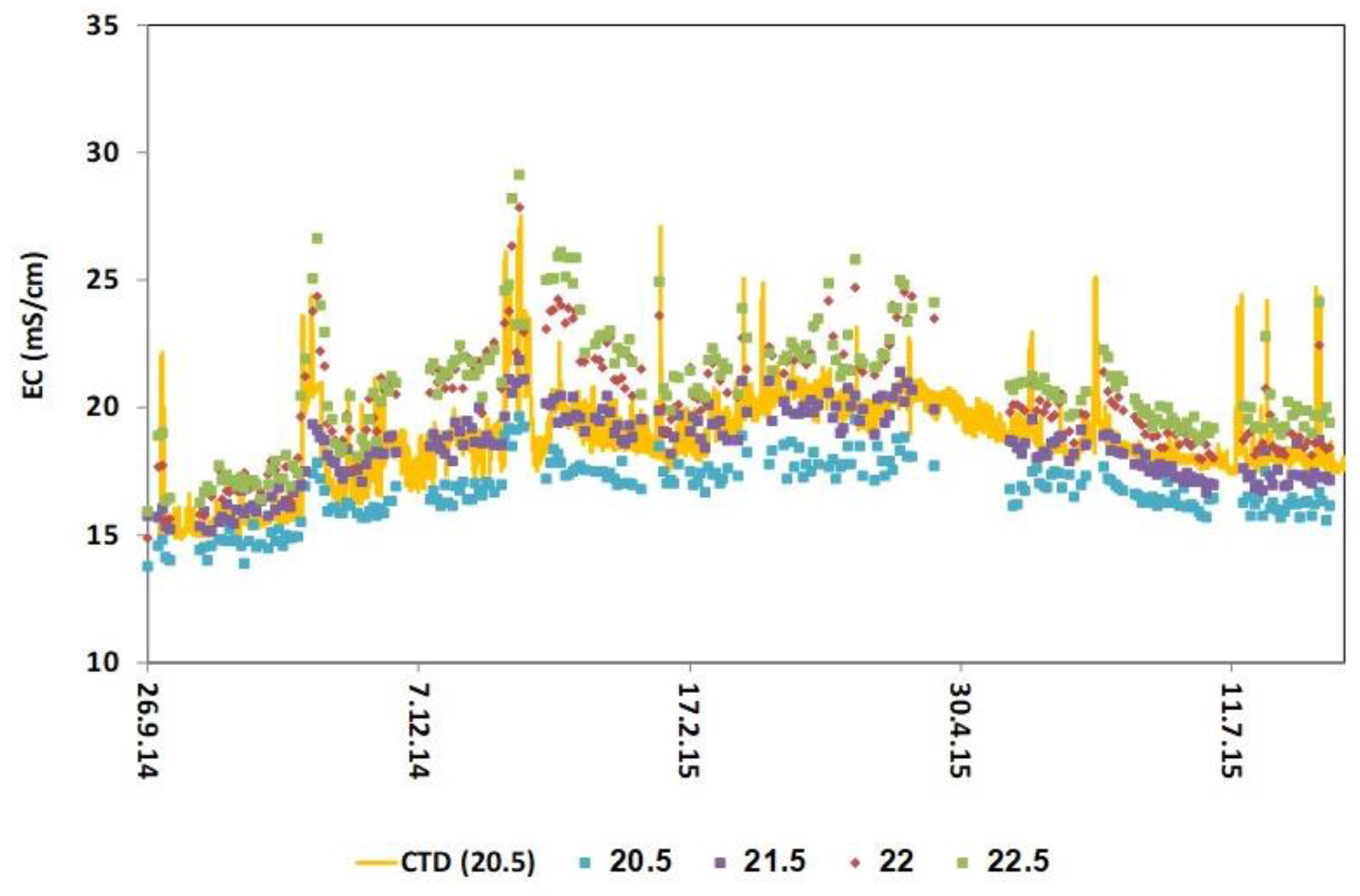In Figure 7 we compare SMD measurements at 20.5–22.5 m depth (1-day frequency) with measurements taken by the CTD diver, which was installed at 20.5 m depth (1-h frequency, −17.5 masl) during September 2014–January 2016. The CTD diver and the SMD generally show similar behavior and trends, again demonstrating the suitability of the SMD method.

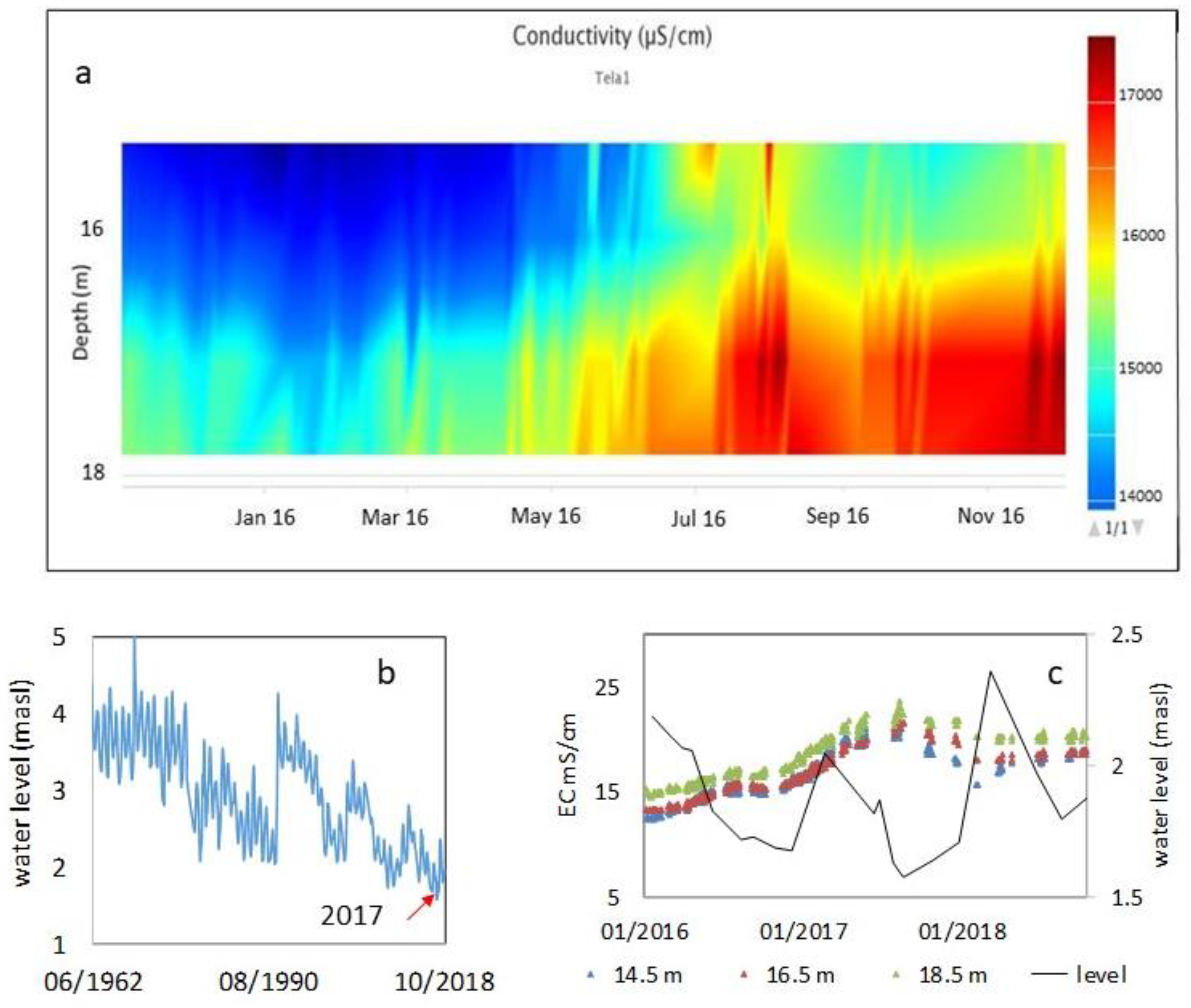
Considering the approved high reliability of the SMD, it can be used to analyze long-term shifts in the location of the interface. This suitability for monitoring FSI displacement is demonstrated in Figure 8a, which is based on daily measurements. A clear trend of increasing salinity between January–December 2016 is observed, documenting an upward shift in the FSI location, which implies that there is an active landward seawater intrusion. We explain this intrusion by historical minimum levels recorded during 2016–2017 in the northern part of the Yarkon Taninim aquifer (Figure 8b), which is the main water source to the confined units of the coastal aquifer in this area [18]. Later measurement from the years 2018 demonstrated that the FSI displacement stopped and even reversed seawards due to a recovery in the Yarkon Taninim level (Figure 8b,c).

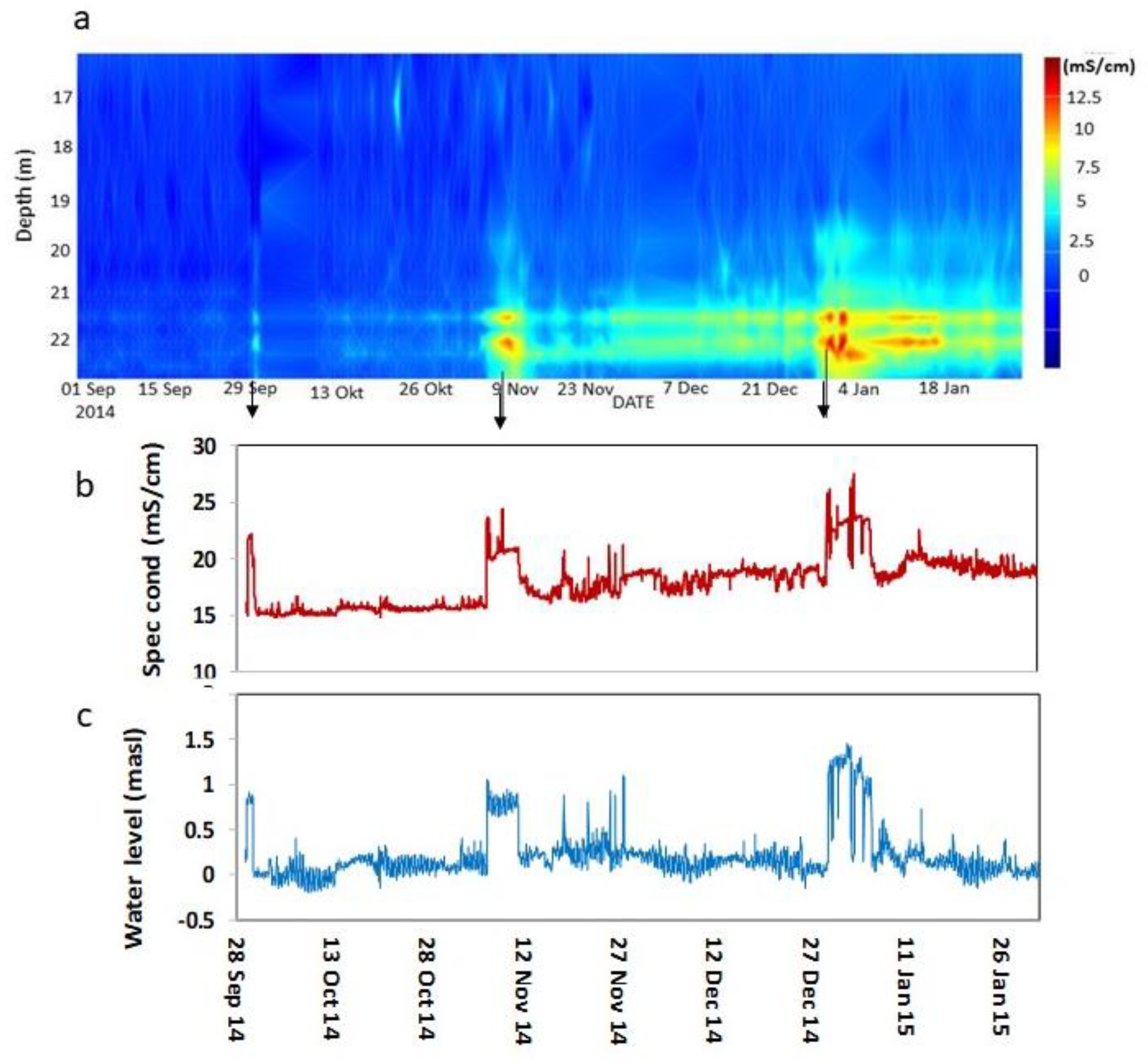
The SMD documented a few transient events of EC increase in the lower 2 m (Figure 9), which were also recorded as an increase of up to 7 mS/cm by the CTD, located at 20.5 m depth (Figure 6 and Figure 8). These were related to pumping breaks in the nearby well P211 (Figure 9), reflected by an increase in water head of about 0.8–1 m during these events (Figure 9). When pumping was renewed, both level and the EC values decreased and restored close to the original values. The increase in salinity when pumping was stopped is hard to explain since the recovery of higher head was expected to push the FSI deeper. We suggest that this has to do with the fact that pumping (the screening part in well 211, Figure 2) is from the bottom, saline, part of the studied unit, which results in preferable withdrawal of saline water and causes FSI deepening. 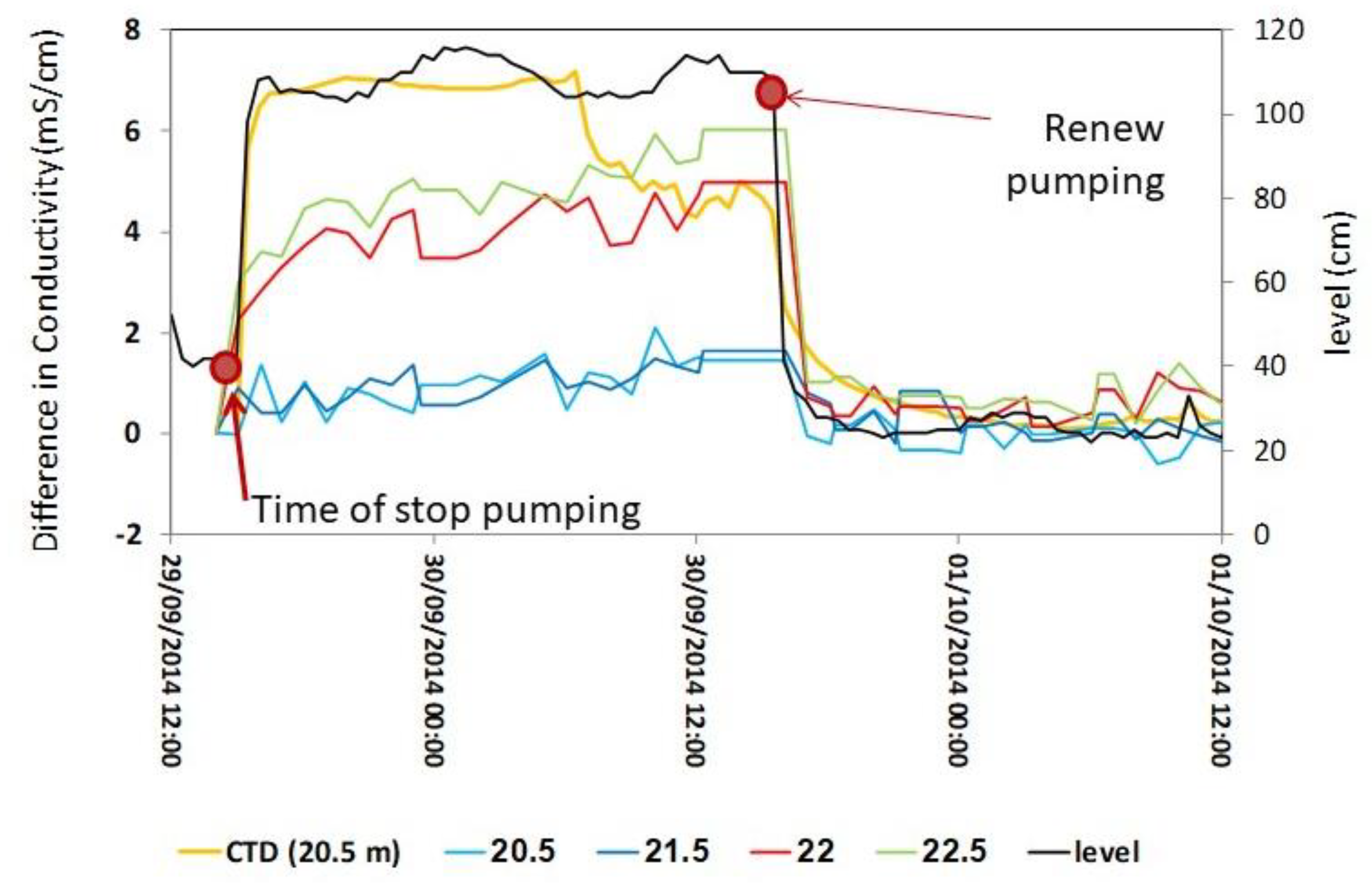This effect is enhanced by the fact that the bottom of unit B is more coarse-grained (shell-rich well log, Geological Survey of Israel, Figure 5), which results in higher conductivity of this part. During pumping breaks, FSI restores to higher levels, while the short nature of these breaks does not allow migration of FSI seawards due to head increase. Another possibility for the changes in salinity could be related to leakage of fresher water from the overlaying unit A (through breaches in the clay) during low heads, while cessation or reduced leakage during pumping breaks, when heads in unit B are significantly higher. This should be further studied. One of the pumping break events was examined in higher time resolution (SMD with 1-h frequency and CTD with 0.5-h frequency, (Figure 10). The EC in both CTD and the SMD increased simultaneously with water level increase, but while the CTD responded immediately and with sharp change in EC (~7 mS/cm within few minutes), the response in the SMD was gradual and the EC changes at 20–22.5 m were 1–6 mS/cm within several hours. We explain this difference by vertical flow in the well [7], which mainly affects the in-borehole measurements of the CTD, but much less so, the wall rock measurements of the SMD. 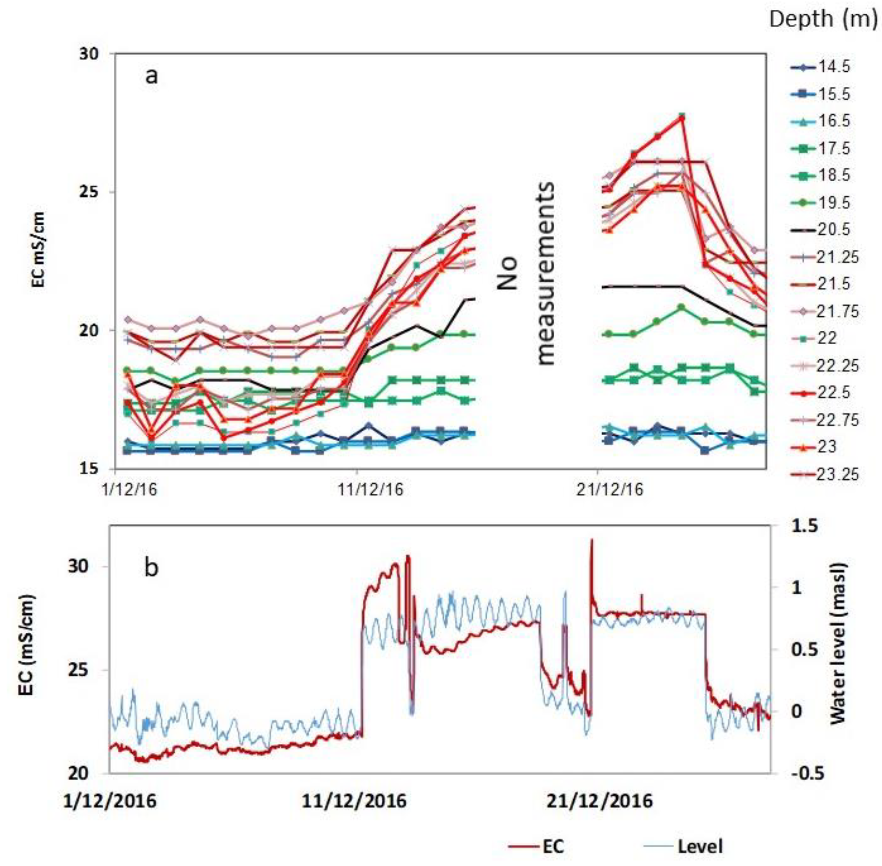The SMD measurements exhibit larger fluctuation in salinity at the deeper part of the well (Figure 10). This may be explained by the shorter spacing between the electrodes (0.25 m), which limits the radial resolution to 13 cm, enhancing the impact of the well vertical flow artefact. A rare opportunity to follow this phenomenon for a longer period of time occurred in December 2016, when the pumping stopped for a few days (Figure 11). While the increase in EC in the CTD records was immediate, in the SMD the EC increased gradually over a few days, demonstrating the slower reaction of the aquifer. The effect of pumping break was also observed farther seawards, in well 72, located 50 m from the sea (Figure 12).

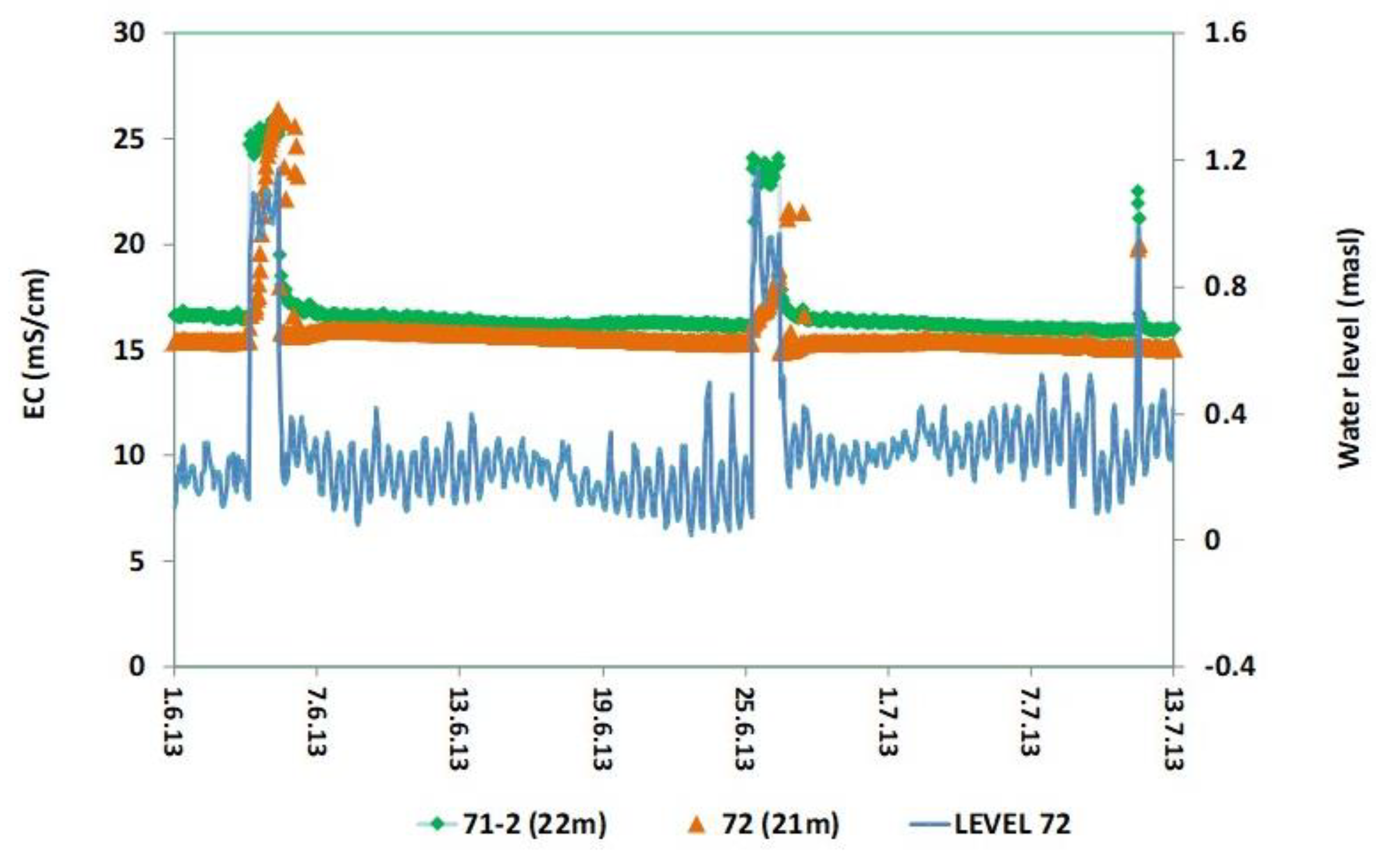
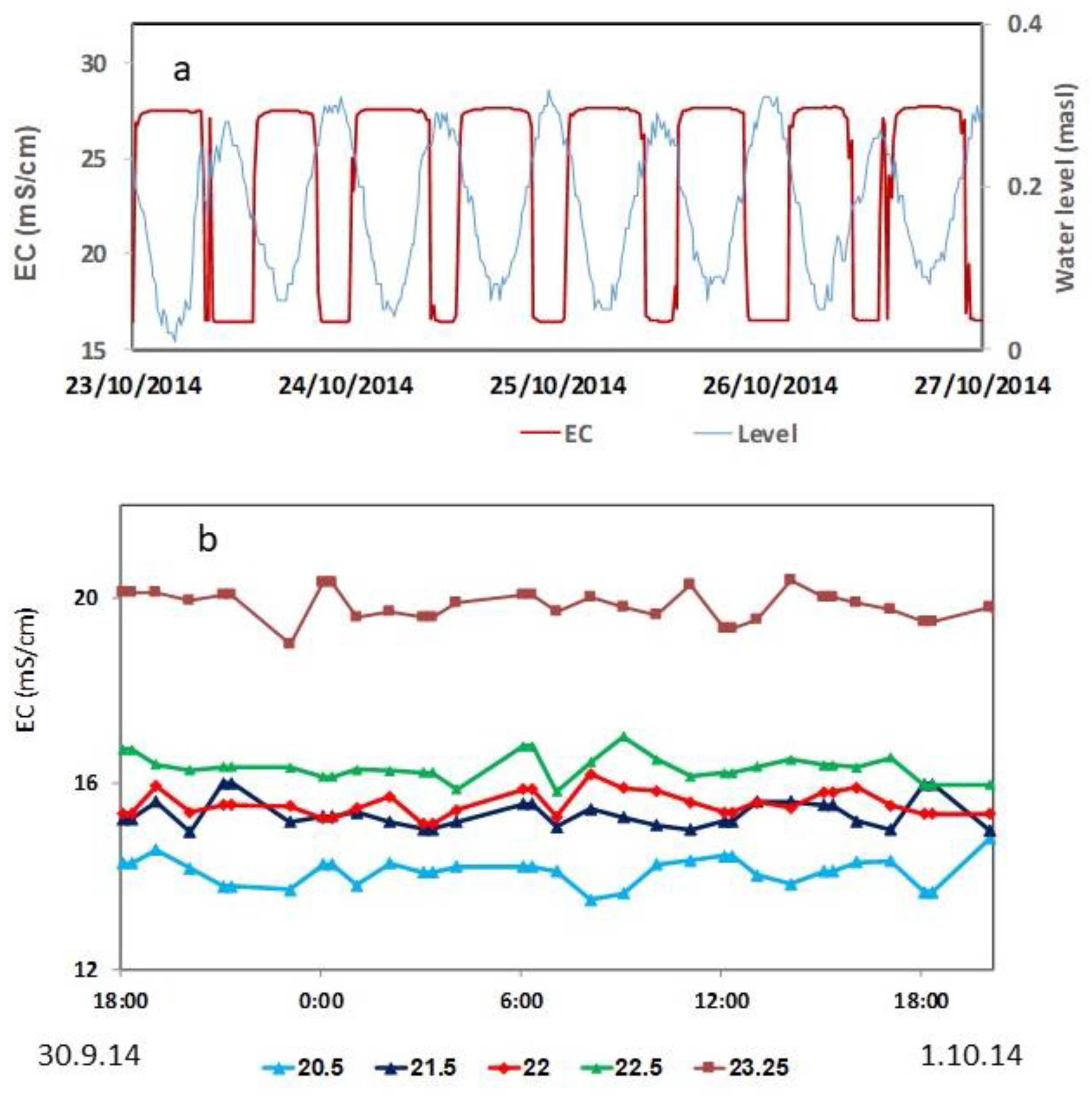
A sharp fluctuation of about 10 mS/cm was observed by CTD in well 72 at depth of 22 m, showing that the FSI also fluctuated in response to sea tide (Figure 13a). Since this fluctuation was not observed by the SMD measurement at depths between 20.5–23.25 m (Figure 13b), which represent the situation in the aquifer and not just in the borehole, it indicates that this observation is related to the phenomena of well artifact [7]. All combined, these observations suggest that the interpretation of common manual profiles of electric conductivity profiles to assess interface shift should be carefully examined, since it may document transient or borehole effects, as was also suggested by previous studies [6,7]. This highlights the need for continuous measurements, using dense arrays of CTD divers or more conveniently, the SMD.

Although we found the SMD tool to be very powerful for monitoring seawater intrusion, we can mention few limitations: In the case of small-scale inhomogeneity (Figure 5), the bulk resistivity is affected by the different rock resistivity and the conversion to water electrical conductivity may be less accurate. This problem does not exist in the common method (RG), since it measures the water conductivity. Detailed drilling stratigraphic data and logging measurements (gamma ray, resistivity and sonic) are needed for very accurate conversion to water conductivity. Those are not always available, especially in an existing old well. Anyway, we found that for pragmatic monitoring, it is not crucial, since we were mainly interested in the change in salinity. The accuracy of the measurement decreases in high salinity (more than sea water) and it is recommended to be used in EC up to 40 mS/cm. Another limitation is the cost, which includes installation and calibration and future yearly cost for maintenance and for visualization and data interpretation tools via a secure web application. In general, this tool is more expensive than the manual EC which is mobile and can be used in other wells. Compare to series of CTD, the SMD is cheaper. The SMD can be installed in slotted PVC with a diameter ranging from 40 mm to 400 mm. In Israel, the monitoring wells are in diameter of 2” which are suitable to SMD. The need to carry a heavy battery and exchange it frequently is another limitation, due to the need for location in an accessible place for a car. This can be solved using solar energy.

Implications to Management of Coastal Aquifers

The data from the SMD can be obtained in real time, and therefore, is more suitable for the management of pumping regime. This is a significant improvement to the common method of EC profiling, which is usually being performed no more than a few times a year and which could lead to wrong interpretation of FSI migration.

Seawater intrusion toward production fields is an ongoing acute problem worldwide. Due to the high salt concentration of the seawater, a very small amount of seawater (2%–3% seawater) can disqualify water for drinking or even irrigating crops. While the process of SWI is usually slow and takes years, this is not always the case, especially when extensive pumping and over-exploitation is involved. Tools like SMD could allow a fast reaction to un-desired SWI displacement—a real-time adjustment of pumping to changing environmental conditions and anthropogenic stresses.

5. Summary and Conclusions

• The problem of seawater intrusion can be monitored in high resolution with the novel SMD (subsurface monitoring device—SMD) method. This method was examined and compared to common methods of CTD (conductivity temperature depth) and electric conductivity profiles (ECP). In general, all methods show similar salinity patterns.
• Pumping effect was clearly monitored with the SMD device, which showed a rise of ~2 m in the transition zone between the saline and the fresh water when pumping was stopped in a nearby pumping well.
• Due to the phenomenon of vertical flow in boreholes, the change in salinity was sharper and faster in the CTD measurement, compared to the SMD, since the first documents the borehole effect, while the latter measures the real FSI shift in the aquifer. This is one of the main advantages of the SMD method.
• The temporary changes in water EC profile may cause error in the interpretation when monitoring with manual ECP (electrical conductivity profile) method, since it is usually done just twice a year. In the SMD method, this problem is overcome because of daily measurements.
• The novel SMD device enables much better FSI monitoring than the existing methodologies. This includes higher frequency profile measurement (compared with the common ECP), monitoring of the ‘real’ SWI displacement in the aquifer rather than in the borehole, and the web-based transfer of data, which provides water managers and policy makers the ability to take decisions in ‘real time’.