Morphological Grayscale Reconstruction and ATLD for Recognition of Organic Pollutants in Drinking Water Based on Fluorescence Spectroscopy

Abstract

This paper proposes a morphological grayscale reconstruction method combined with an alternating trilinear decomposition (ATLD) and threshold method based on 3D fluorescence spectroscopy to detect pollutants present at low concentrations in drinking water. First, the morphological grayscale reconstruction method was used to locate the fluorescence peaks of pollutants by comparing the original and reconstructed spectra obtained through expansion. The signal in the characteristic spectral region was then enhanced using an amplification factor. Feature extraction was subsequently performed by ATLD, and the threshold method was used to qualitatively distinguish water quality. By comparing the proposed method with the direct use of the ATLD and threshold method—which is a commonly used feature-extraction method—this study found that the application of the morphological grayscale reconstruction method can extrude characteristics of 3D fluorescence spectra. Given the typical spectral characteristics of phenol, salicylic acid, and rhodamine B, they were selected as experimental organic pollutants. Results illustrated that the morphological grayscale reconstruction with ATLD improved the spectral signal-to-noise ratio of pollutants and can effectively identify organic pollutants, especially those present at low concentrations.

1. Introduction

Drinking water is the kind of resource that affects all aspects of public life. When its safety is threatened, it may pose public health risks that will lead to environmental and socio-economic losses [1]. Even at low concentration and short exposure, organic pollutants can still cause acute poisoning. With the widespread use of organic compounds, water-pollution incidents keep increasing, and the influential range and degree become wilder and more serious [2]. Therefore, quickly alerting and effectively identifying possible water-pollution events in the water supply system are essential tasks.

Many researchers have proposed many kinds of methods to detect water quality information because water quality has been increasingly paid attention by the world, and the detection technology becomes more urgently needed. Chemical analysis [3], gas chromatography (GC) [4], high-performance liquid chromatography (HPLC) [5,6], and gas chromatography-mass spectroscopy (GC/MS) [7] are common methods for water-quality detection, although they are complex and time-consuming. The concentration of pollutants is generally low after contaminant intrusion takes place in urban water supply systems, and according to the Environmental Health Criteria-EHC 161 [8] and the ‘Guidelines for drinking water quality standards in developing countries’ [9], the concentration limit of most organic pollutants is below 10 μg/L. Therefore, it is important to develop a detection technology for organic pollutants in drinking water with highly effective detection ability, so that pollution events can be detected in a timely manner and the pollutant can be accurately identified. Spectral analysis—as a new detection method without sample extraction, enrichment, other pretreatments, and chemical reagent addition—is gaining increased attention in the field of water-quality detection [10]. Common spectral analysis methods include UV-Vis and fluorescence spectroscopy [11,12,13,14,15]. UV-Vis detection has a certain boundedness in terms of sensitivity and detection limit. By contrast, 3D fluorescence spectroscopy can play an important role in the detection and analysis of organic pollutants in drinking water because it has multiple advantages such as high comprehensive characterization and abundant fluorescence information, high sensitivity, fast detection speed, and good selectivity.

The steps of detecting organic pollutants in drinking water generally include preprocessing of 3D fluorescence spectrum, feature extraction, and the classification and identification of organic pollutants [16]. Li et al. [17] proved that the Tchebichef moment method can independently extract quality information of the target compound by fully using its multi-resolution capability and obtained accurate quantitative analysis results even if severely overlapping signals existed. Nicolas et al. [18] investigated the predictability of disinfection by-products (DBPs) with low concentration in drinking water using fluorescence data coupled with neural networks and revealed that this method can improve prediction accuracy. Huang et al. [19] utilized 2D Gabor wavelet coupled with block statistics to extract the 3D fluorescence spectral characteristics of drinking water and used support vector machine (SVM) for multi-classification and identification of pollutants with closely positioned or overlapping peaks. Stedmon [20] modeled using PARAFAC for monitoring contamination events, and the results of this study suggest that contamination could be detected at levels equivalent to the addition of 60 mg C/L in drinking water with a total organic carbon (TOC) concentration of 3.3 mg C/L. Alternating trilinear decomposition (ATLD), an improved method of PARAFAC [21] with its advantages of being insensitive to an overestimated component number, being robust and having fast convergence. Dong-MeiFang [22] proposed ATLD and PARAFAC for simultaneous direct determination of ofloxacin (OFL), norfloxacin (NOR), and enoxacin (ENO) and results by using ATLD with an estimated component number of five were more acceptable for clinical analysis. Jie Yu [23] proposed a qualitative analysis approach to detect water contamination events with unknown pollutants based on ATLD. Huan-Bo Wang [24] accomplished determination of five polycyclic aromatic hydrocarbons by 3D fluorescence coupled based on ATLD, and this method was also employed for the determination of samples of drinking water spiked with all these Polycyclic Aromatic Hydrocarbons (PAHs). The results were not as satisfying as those in synthetic samples due to the negative effects of humic acid or fulvic acid in drinking water. Researchers have explored qualitative discrimination, quantitative analysis, and classification and identification based on 3D fluorescence spectra. However, the detection rate (ratio of the number of organic pollutants that are recognized correctly to the total number of organic pollutants) of organic pollutants present in low concentrations can still be improved in the context of background drinking water fluctuating constantly.

This study introduced the morphological grayscale reconstruction method to extrude characteristics of 3D fluorescence spectra. The morphological method is common in the field of image analysis, which has been widely applied in various fields of image processing and is an effective image feature extraction technology [25]. The structure of 3D fluorescence spectrum is similar to that of a gray image. Each spectral point in an EEM data can be regarded as a pixel of the image, whereas the characteristic peak of the spectrum corresponds to the common ‘dome’ in morphology. Gu et al. [26] proposed a new detection algorithm for infrared dim and small targets using saliency and grayscale morphological reconstruction. Zhang et al. [27] applied a morphological method to obtain the location of peaks in 2D fluorescence, which made the identification of two pesticides in tea liquor via peak point matching possible.

In the real-time monitoring process of water quality with the application of fluorescence spectroscopy, the detection rate of organic pollutants at low concentrations is a problem. This work describes the novel use of morphological grayscale reconstruction method in 3D fluorescence spectra to locate spectral features and amplify the signal with an amplification factor, then realizes the feature extraction using the alternating trilinear decomposition method (ATLD) and completes the qualitative discrimination of water quality by combining threshold methods.

2. Materials and Methods

2.1. Solution of Organic Pollutants

Rhodamine B is a material used to produce fluorescent dyes, Salicylic acid is a matter that may produce a large amount of wastewater, Phenol is a common industrial raw material. They have caused contamination events in the past, for example, on 26 April 2018, 20 people suffered from a phenol leak at a chemical plant in the Czech Republic; on 18 June 2018, phenol has leaked from a tanker truck that met with an accident at Kuthiran, the odor of the chemical was experienced in a canal 5 km away, fish fatalities occurred, and the use of drinking water was restricted.

In this paper, various concentrations of phenol, salicylic acid, and rhodamine B solutions were prepared with tap water. The detection limits are 0.1 μg/L, 0.35 μg/L and 0.22 μg/L respectively. We aimed at improving recognition rate of organic pollutants at low concentrations when drinking water was the background solution. The conductivity of tap water is between 125 and 1250 μs/cm, dissolved organic carbon (DOC) is an index to assess both the water quality of tap water and if there is any fluorescent dissolved organic matter, such as protein-like and humic-like organic matter. Samples preparation were done as follows:

(1)

Preparation of stock solution: Stock solutions (0.1 g/L) of phenol, salicylic acid, and rhodamine B were prepared by dissolving 0.1 g in 1 L tap water. The solutions were stored in the dark.

(2)

Preparation of working solution: Separate stock solutions (1 mL) of phenol, salicylic acid, and rhodamine B were placed in 1 L volumetric flask and made up to volume, resulting in 100 μg/L solution. Then, 2, 4, 6, 8, 10, 20, 30, and 40 mL solution were collected from the 100 μg/L solution and prepared into 2, 4, 6, 8, 10, 20, 30, and 40 μg/L solutions with tap water, respectively.

2.2. Fluorescence Spectroscopy

Experiments were conducted using Hitachi F-4600 fluorescence spectrometer. The excitation and emission wavelengths ranged from 200 nm to 700 nm, the scanning interval was 5 nm, the scanning speed was 12,000 nm/min, the slit width was 10 nm, the PMT voltage was 700 V and the sample was measured in a 1 cm × 1 cm × 4.5 cm quartz fluorescence cuvette.

2.3. Morphological Grayscale Reconstruction

Information on 3D fluorescence spectrum was obtained using morphology by constantly moving structural elements. When structural elements moved, the structural features of each region were continuously acquired [28]. For a point $f(x,y)$ in the data of 3D fluorescence were the basic operations of grayscale morphology were corrosion and expansion:

$$(f\mathsf{\Theta }g)(x,y)=\underset{i,j}{min}\{f(x-i,y-j)-g(-i,-j)\}$$

(1)

$$(f\oplus g)(x,y)=\underset{i,j}{max}\{f(x-i,y-j)+g(i,j)\},$$

(2)

where $f$ is the grayscale information of the spectrum, $g$ is the grayscale information of structural elements, and $g(i,j)$ represents the structural elements. The expression of grayscale morphological expansion and morphological corrosion operation are very similar to the convolution integral [29]. Grayscale morphological expansion is a process of data expansion, whereas the corrosion operation is a process of data reduction.

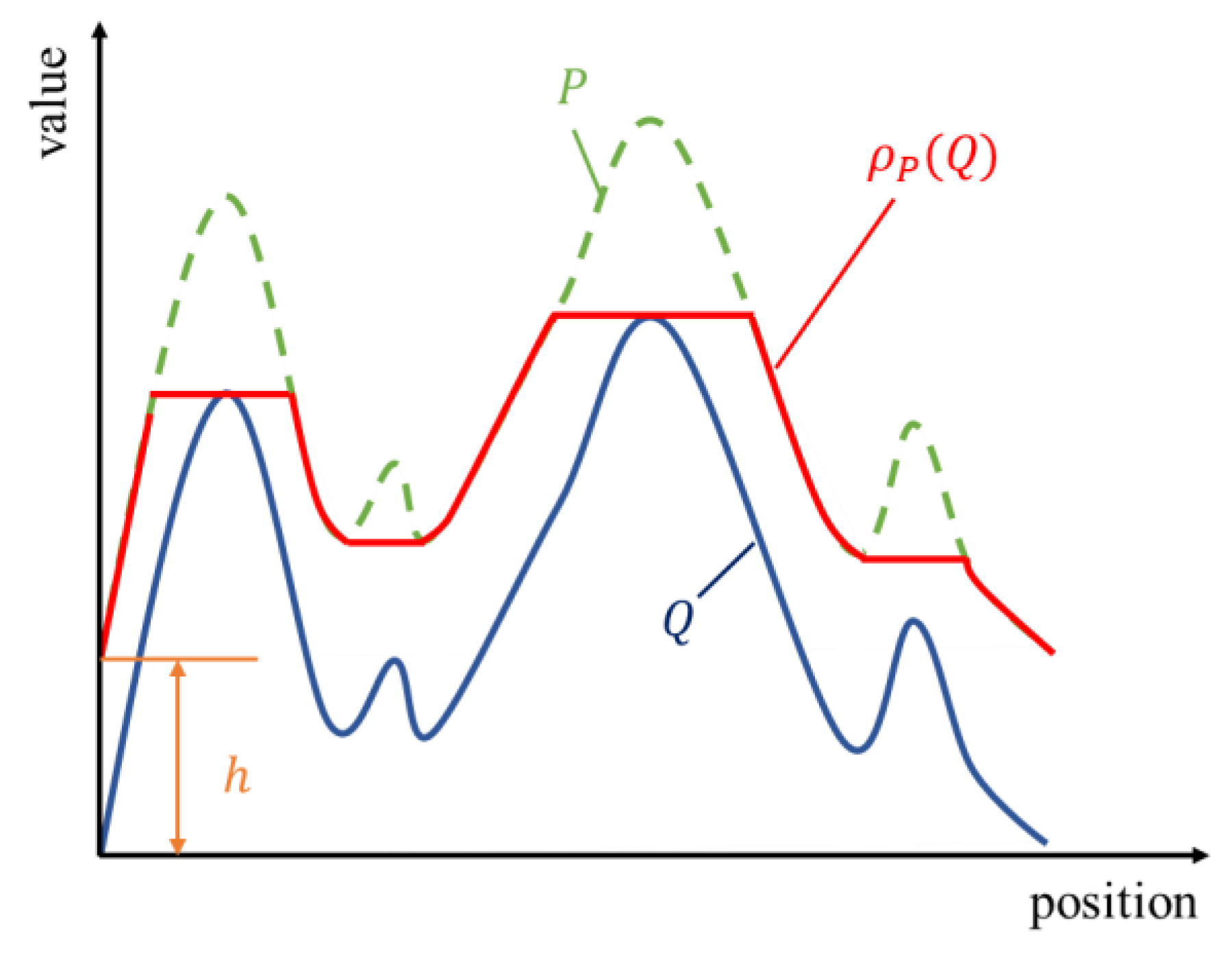
The basic principle is shown in Figure 1. In the figure, $P$ represents the original spectrum, $Q$ represents the marked spectrum, ${\rho }_P(Q)$ represents the reconstructed spectrum, and the marked spectrum was obtained by subtracting a constant h from its original spectrum, namely $Q=P-h$. The position of all ‘domes’ was obtained according to the difference of spectroscopy before and after reconstruction. The domes of spectrum $P$ are denoted as $dom{e}_h(P)$, the value of each point is the difference between the value of each point in spectrum $P$ and the value of the corresponding point in the reconstruction result ${\rho }_P(Q)$, that is $dom{e}_h(P)=P-{\rho }_P(P-h)$. A ‘dome’ is an area with large local gray value in spectroscopy $P$. When h is equal to 1, the dome of the spectroscopy is only the region with the maximum value. The characteristic peak information of 3D fluorescence spectrum was screened from these extracted ‘dome’ structures.

The reconstructed spectrum ${\rho }_P(Q)$ is realized by expansion operation. Vincent [30] proposed that morphological reconstruction can be achieved by repeating expansion of $Q$ on the premise that the gray level does not exceed $P$. The basic expansion ${\delta }_P^{(1)}(Q)$ of the spectroscopy Q can be defined as:

$${\delta }_P^{(1)}(Q)=(Q\oplus g)\wedge P$$

(3)

where $g$ denotes a structural element, $Q\oplus g$ denotes an expansion operation of $Q$ with $g$, $\wedge$ denotes that the expansion result compared with $P$ point by point, and the minimum value can be obtained after comparison. Then $n\left(n\ge 0\right)$ times basic expansion of $Q$ can be expressed as:

$${\delta }_P^{(n)}(Q)=\underset{n}{\underbrace{{\delta }_P^{(1)}{\delta }_P^{(1)}\cdots {\delta }_P^{(1)}}}(Q)$$

(4)

${\delta }_P(Q)={\vee }_{n\ge 1}{\delta }_P^{(n)}(Q)$ was the reconstruction result of spectrum $P$ with the structural element $g$, and $\vee$ represents comparing ${\delta }_P^{(1)}(Q),{\delta }_P^{(2)}(Q),\cdots \cdots ,{\delta }_P^{(n)}(Q)$ point by point and taking the maximum value.

2.4. Alternating Trilinear Decomposition

Assuming that the number of samples measured is $K$, the number of excitation wavelengths is $I$, and the number of emission wavelengths is $J$, the 3D fluorescence spectral matrix $X$ (EEMs) obtained by this detection can be expressed as [21]:

$$X_{ijk}={\displaystyle \sum _{n=1}^N{a}_{in}{b}_{jn}{c}_{kn}}+e_{ijk}$$

(5)

where $N$ represents the number of factors actually contributing to fluorescence, $x_{ijk}$ is an element in the 3D fluorescence spectral matrix $X$, which represents the fluorescence intensity of sample $k$ at an excitation wavelength of $i$ and emission spectrum of $j$, $c_{kn}$ is an element in the relative concentration matrix $C(K\times N)$, $a_{in}$ is an element in the relative excitation matrix $A(I\times N)$, $b_{jn}$ is an element in the relative emission matrix $B(J\times N)$, and $e_{ijk}$ is an element in the 3D residual matrix $E$.

In order to adapt to the trilinear model, Harshman [31] proposed to adopt the sum of squared residuals (SSR) as the loss function to represent the difference between real and trilinear decomposition data, which can be expressed as:

$$SSR={\displaystyle \sum _{i=1}^I{\displaystyle \sum _{j=1}^J{\displaystyle \sum _{k=1}^K{(x_{ijk}-{\displaystyle \sum _{n=1}^N{a}_{in}{b}_{jn}{c}_{kn}})}^2}}}$$

(6)

ATLD [21] improves the performance of trilinear decomposition in alternating iterative operations based on the Moore–Penrose step in singular value decomposition (SVD). Matrices A, B, and C were solved according to the following iterations:

$$a_{(i)}^T=diag(B^{+}{X}_{i\mathrm{..}}{(C^T)}^{+})$$

(7)

$$b_{(j)}^T=diag(C^{+}{X}_{.j.}{(A^T)}^{+})$$

(8)

$$c_{(k)}^T=diag(A^{+}{X}_{\mathrm{..}k}{(B^T)}^{+})$$

(9)

where $i=1,2,\dots I;j=1,2,\dots J;k=1,2,\dots K$, $diag(\cdot )$ means to take the diagonal elements of the matrix as a column of vectors. $A^{+},B^{+},C^{+}$ represent the Moore–Penrose generalized inverse of $A,B,C$, respectively. $a_{(i)}^T,b_{(j)}^T,c_{(k)}^T$ respectively denote the transpose of the $i$ th row vector of relative excitation matrix $A$, the $j$ th row vector of relative emission matrix $B$, and the $k$ th row vector of relative concentration matrix $C$. During each iteration, matrices $A$ and $B$ are normalized to unit length by column.

The 3D fluorescence spectral data of drinking water were processed according to the principle of ATLD algorithm. First, the sample data set of drinking water $W_{I\times J\times K}$ (the number of drinking water samples is $K$, excitation wavelength number is $I$, and emission wavelength number is $J$) were obtained with ATLD and modeling and included model parameters, such as relative excitation matrix $A$, relative emission matrix $B$, and the relative concentrations matrix of components $C$.

Substituting $A,B,C$ into Formula (1), the estimated spectral matrix of background drinking water ${\widehat{W}}_{I\times J\times K}$ was acquired. The measured value of 3D fluorescence spectral matrix of the background drinking water sample $W_{I\times J\times K}$ was compared with the estimated value ${\widehat{W}}_{I\times J\times K}$ to obtain a residual matrix $U_{I\times J\times K}$:

$$U_{I\times J\times K}=W_{I\times J\times K}-{\widehat{W}}_{I\times J\times K}$$

(10)

The sum of the squares of each element in each residual matrix $u_{ijk}$ was calculated to obtain the SSRs of drinking water $ss{r}_k$:

$$ss{r}_k={\displaystyle \sum _{j=1}^J{\displaystyle \sum _{i=1}^I{u}_{ijk}}}.$$

(11)

The mean $\overline{x}$ and variance $\sigma$ of all SSRs $ss{r}_k(k=1,2,3\dots ,K)$ were found.

According to the principle of three standard deviations, the threshold $q$ is:

$$q=\overline{x}\pm 3\sigma .$$

(12)

The measured value of 3D fluorescence spectral matrix $X_{I\times J}$ of the sample under test was obtained after preprocessing:

$$X_{I\times J}={\displaystyle \sum _{n=1}^N{a}_{in}{b}_{jn}{c}_n+e_{ij}}$$

(13)

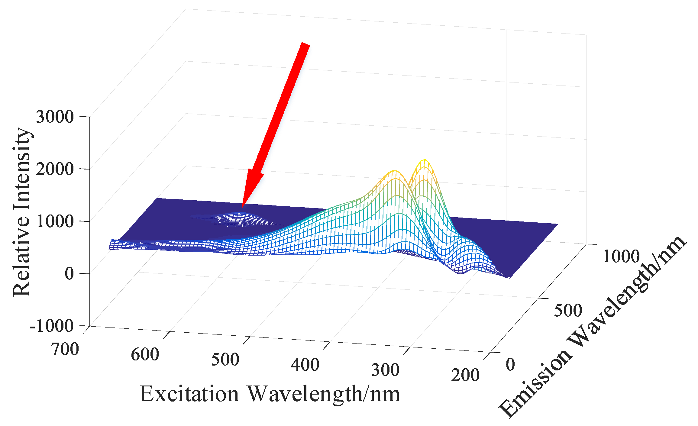
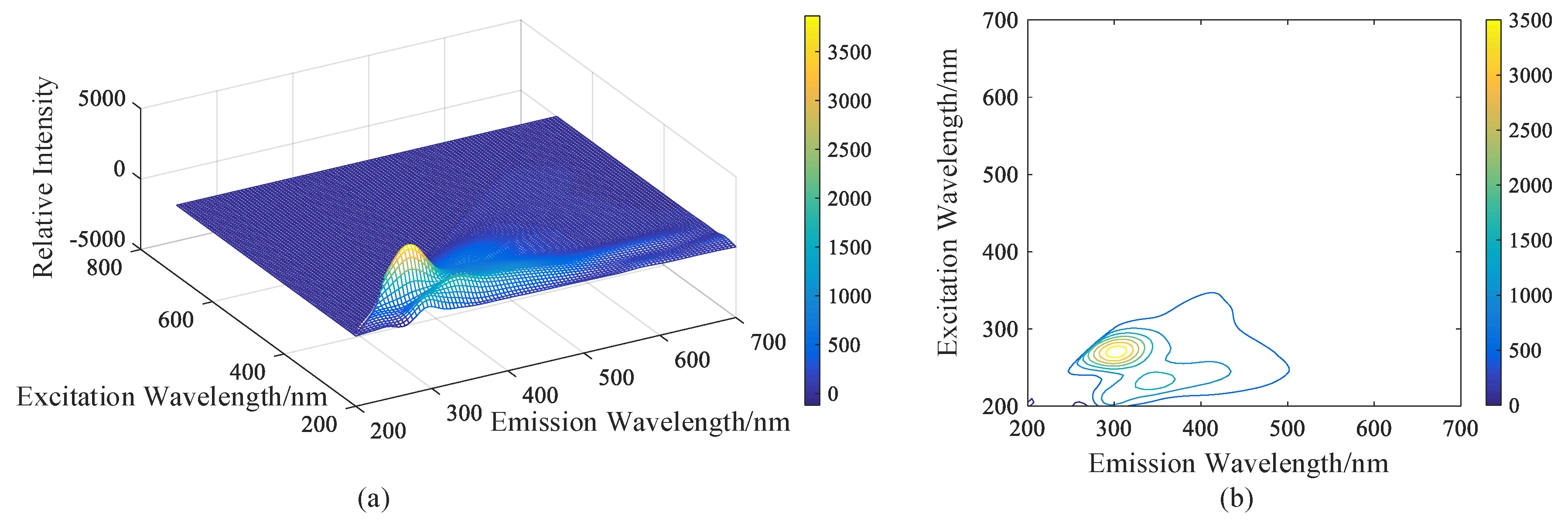
where $N$ is the number of components. For background drinking water, its 3D fluorescence spectrum has two distinct characteristic peaks, so the number of components $N$ is 2. $c_n$ is the element in the relative concentration matrix $C$, indicating the relative concentration of the $n$ th component. $a_{in}$ is the element in the relative excitation matrix $A(I\times N)$. $b_{jn}$ is the element in the relative emission matrix $B(J\times N)$. $e_{ij}$ is the element in the 3D residual matrix $E$. Substituting $A,B$, and EEM matrix $X_{I\times J}$ of the sample under test into Formula (5), the estimated relative concentration matrix $\widehat{C}$ of each component of the sample under test was obtained. Substituting $A,B,\widehat{C}$ into Formula (1), the estimated value of the 3D fluorescence spectral matrix of the sample under test was ${\widehat{X}}_{I\times J}$. $E_{I\times J}$ can be represented by comparing the estimated value ${\widehat{X}}_{I\times J}$ and the measured value $X_{I\times J}$ is:

$$E_{I\times J}={\widehat{X}}_{I\times J}-X_{I\times J}$$

(14)

The $SSRX$ is the sum of each element in $E_{I\times J}$:

$$SSRX={\displaystyle \sum _{j=1}^J{\displaystyle \sum _{i=1}^I{e}_{ij}}}.$$

(15)

By comparing the $SSRX$ of the sample under test with the threshold $q$, it can be effective in discriminating pollutant samples from the normal water samples.

3. Results

3.1. Fluorescence Spectral Characteristics of Pollutants with Different Concentrations

Based on the theory of fluorescence, different concentrations of organic pollutants generate difference fluorescence intensities. High concentration samples contain more fluorescence reactive substances, so the corresponding characteristic fluorescence intensity is more obvious. Meanwhile, low concentration samples contain traces of fluorescence reactive substances, resulting in weak fluorescence characteristic intensity. The drinking water solutions containing salicylic acid, rhodamine B, and phenol were divided into high and low concentration groups. Those with concentrations higher than 10 μg/L were placed into the high concentration group, whereas those with concentrations lower than 10 μg/L were placed into the low concentration group. The experimental grouping is shown in

Table 1. Grouping of experimental pollutants.

Group	High Concentration Group (μg/L)	Low Concentration Group (μg/L)
A	A1: 10, 20, 30, 40	A2: 2, 4, 6, 8
B	B1: 10, 20, 30, 40	B2: 2, 4, 6, 8
C	C1: 10, 20, 30, 40	C2: 2, 4, 6, 8
D	D1: 10, 20, 30, 40	D2: 2, 4, 6, 8

. The samples tested were background drinking water samples in groups A and B, and samples in group A were collected from tap water on one day, while samples in group B were collected on another day. Meanwhile, samples in group C were collected on consecutive days, while samples in group D were collected on other consecutive days.

Figure 2, Figure 3 and Figure 4 show the 3D fluorescence spectra of salicylic acid, rhodamine B, and phenol drinking water solutions, respectively, at 40, 10, and 4 μg/L. At 40 μg/L, the 3D fluorescence spectra of the three pollutants had obvious fingerprint characteristics. Small red dots in figures are used to point out the peaks. Salicylic acid had three characteristic peaks. One characteristic peak was observed at 290–300/400–410 nm in excitation band/emission band, whereas the other two overlap with that of drinking water, which was caused by the superposition of fluorescence spectra. The characteristic peak of rhodamine B was observed at 555/570–580 nm in excitation band/emission band, and that of phenol was observed at 270–280/305–315 nm in excitation band/emission band, which overlapped with that of drinking water. With a decreased concentration of the three pollutants, the fluorescence intensity of their characteristic peaks decreased. Texture, characteristic peak position, and characteristic peak intensity can be used to measure the similarity of the fluorescence spectroscopy. At 4 μg/L, the 3D fluorescence spectrum of the polluted drinking water solution was close to that of drinking water itself. Therefore, for an online monitoring system of drinking water, effective methods of feature extraction and abnormal detection methods are very important to detect organic pollutants.

3.2. Qualitative Discrimination Results Based on Morphological Grayscale Reconstruction and ATLD

Figure 5 is the 3D fluorescence spectra of 2 μg/L rhodamine B. The characteristic peaks of rhodamine B can be observed; however, due to the fluctuation of the background water sample, they can easily be confused with the background water sample and cannot be detected accurately. Thus, morphological grayscale reconstruction is introduced to enhance the characteristic peaks.

The drinking water samples of groups A and B were decomposed with ATLD to obtain relative excitation matrix $A$, relative emission matrix $B$, and relative concentration matrix $C$. Considering that the 3D fluorescence spectrum of drinking water contains two characteristic peaks, the number of factors set in the algorithm was two. The relative excitation matrix and relative emission matrix of different factors are shown in Figure 6.

The qualitative discrimination results of different groups based on the improved algorithm before and after are shown in

Table 2. Qualitative discrimination results of groups A and B without improved algorithm.

	Real	Drinking Water	Salicylic Acid	Rhodamine B	Phenol
Prediction
Drinking water		40	4	10	6
salicylic acid		0	29	0	0
rhodamine B		0	0	24	0
phenol		0	0	0	28

,

Table 3. Qualitative discrimination results of groups A and B without improved algorithm

	Real	Drinking Water	Salicylic Acid	Rhodamine B	Phenol
Prediction
Drinking water		40	8	10	13
salicylic acid		0	24	0	0
rhodamine B		0	0	23	0
phenol		9	0	0	20

,

Table 4. Qualitative discrimination results of groups A and B based on the improved algorithm.

	Real	Drinking Water	Salicylic Acid	Rhodamine B	Phenol
Prediction
Drinking water		40	2	0	8
salicylic acid		0	31	0	0
rhodamine B		0	0	34	0
phenol		0	0	0	26

and

Table 5. Qualitative discrimination results of groups C and D based on the improved algorithm

	Real	Drinking Water	Salicylic Acid	Rhodamine B	Phenol
Prediction
Drinking water		40	0	3	11
salicylic acid		0	32	0	0
rhodamine B		0	0	30	0
phenol		0	0	0	22

.

As presented in

Table 6. Qualitative discrimination results based on the improved algorithm.

Classification	A	B	C	D	Totals
total number of samples	67	74	68	70	279
sample number of drinking water	20	20	20	20	80
sample number of organic pollutants	47	54	48	50	199
detection number of pollutants	43	48	41	43	175
detection rate of pollutants (%)	91.5	88.9	85.4	86	87.9
false alarm number	0	0	0	0	0
false alarm rate (%)	0	0	0	0	0

,

Table 7. Qualitative discrimination results without the improved algorithm.

Classification	A	B	C	D	Totals
total number of samples	67	74	68	70	279
sample number of drinking water	20	20	20	20	80
sample number of organic pollutants	47	54	48	50	199
detection number of pollutants	35	46	30	37	148
detection rate of pollutants (%)	74.5	85.2	62.5	74	74.4
false alarm number	0	0	0	0	0
false alarm rate (%)	0	0	0	0	0

,

Table 8. Qualitative discrimination results of different concentrations based on the improved algorithm.

Classification	A1	A2	B1	B2	C1	C2	D1	D2
total number	23	24	24	30	24	24	26	24
detection number	23	20	24	24	24	17	26	17
detection rate (%)	100	83.33	100	80	80	70.83	100	70.83

and

Table 9. Qualitative discrimination results of different concentrations without the improved algorithm.

Classification	A1	A2	B1	B2	C1	C2	D1	D2
total number	23	24	24	30	24	24	26	24
detection number	22	13	24	22	23	7	25	12
detection rate (%)	95.65	54.17	100	73.33	95.83	29.17	96.15	50

, after the enhancement of the characteristic signals, the detection rate of overall organic pollutants was 87.9%, which was 13.5% higher than previously detected. For the high concentration group, all samples can be detected, and the detection rate obviously improved. As Table 4 and Table 5 have shown specifically, for the low concentration groups A2 and B2, the average detection rate of the original qualitative discrimination method was 64.8%, whereas the average detection rate after morphological feature extraction and signal enhancement was 81.5%, showing obvious improvement. For the low concentration groups C2 and D2, the average detection rate of the original method was 39.6%, whereas the average detection rate of the improved method was 70.8%. The detection accuracy improved by nearly two times.

4. Discussion

The ability to locate spectral characteristic peak positions depend on whether the signal of the relevant spectral region can be correctly amplified, which is important in pollutant detection. In this paper, taking the samples under test in groups A and B as an example, peak localization of representative concentration solution of each pollutant group was performed. The characteristic peaks of drinking water were removed to reduce their influence. The characteristic peak positions of 20 and 4 μg/L salicylic acid and 20 and 4 μg/L rhodamine B and phenol solution were obtained using the morphology grayscale reconstruction method. Figure 7, Figure 8, Figure 9, Figure 10 and Figure 11 show the localization results of characteristic regions of fluorescence spectra of various pollutant samples with different concentrations.

The morphological grayscale reconstruction algorithm was used to further extract features from the spectrum and amplify the signal in the region of characteristic spectrum with an amplification factor. As the 3D fluorescence spectrum of drinking water contains two characteristic peaks, the number of factors in the algorithm was set to two. The modeling results and residual matrix of drinking water are shown in Figure 12. Taking 4 μg/L rhodamine B as an example, modeling results and residual matrix of the measured sample based on the original method are shown in Figure 13, and those based on the improved method are shown in Figure 14.

Figure 12, Figure 13 and Figure 14 show that the residual error matrix has obvious data in the characteristics of the area after feature enlargement. For rhodamine B, 4 μg/L was low such that it was easily interfered with by other noise signals when calculating the residual value, thus, key information of the characteristic peaks was lost. Through the method proposed in this paper, the spectral signal-to-noise ratio and the detection efficiency of pollutants were improved.

In practical applications, we need to encapsulate our algorithms and deploy them to the server. After obtaining fluorescence data, the server with CPU and memory would call the algorithms automatically and identify contaminants in drinking water.

5. Conclusions

From the experimental results above, ATLD, which is a common fluorescence spectral feature extraction and modeling algorithm method, can achieve good detection effect when used in the detection of pollutants at high concentrations in drinking water. However, when the concentration of organic pollutants was low, especially when the background water quality was fluctuating greatly, the detection of this method would be affected, such as the concentration of rhodamine B below 10 μg/L and the concentration of phenol and salicylic acid below 6 μg/L. The feature-extraction method based on morphology grayscale reconstruction combined with ATLD was proposed in this paper. Emission wavelength/excitation wavelength of 3D fluorescence spectral characteristic peaks can be acquired by expansion operations in the morphological grayscale reconstruction method, so that the effective localization of the characteristic peak can be realized. A certain size of amplification factor was set so that the area of data can be weighted, then the characteristics of the signal which was weak and easily ignored can be singularized. The organic pollutants had obvious data in the characteristic area after morphological grayscale reconstruction, which was vividly contrasted by 3D fluorescence spectra of normal drinking water samples, leading the SSR values of residual matrix deviating from the normal range through ATLD modeling. As a result, abnormal samples are properly identified, and the detection rate of organic pollutants present at low concentration is improved, with the concentration of rhodamine B and salicylic acid above 2 μg/L almost be detected.

Although the methodology has a relatively low detection rate, the detection effect of phenol almost has no ascension because the characteristic peaks of drinking water are removed while characteristic peaks position of phenol overlaps that of drinking water, so that the characteristic spectrum area of phenol is not amplified. Additional studies should be carried out in order to further decrease the detection rate of those pollutants having overlapping peaks with drinking water present at low concentrations.

In summary, given the above advantages, this method shows great promise and can be used in water-quality detection with 3D fluorescence spectroscopy and ensure public health.

References

1. Arnon, T.A.; Ezra, S.; Fishbain, B. Water characterization and early contamination detection in highly varying stochastic background water, based on Machine Learning methodology for processing real-time UV-Spectrophotometry. Water Res. 2019, 155, 333–342. [Google Scholar] [CrossRef]
2. Asquith, E.; Evans, C.; Dunstan, R.H.; Geary, P.; Cole, B. Distribution, abundance and activity of geosmin and 2-methylisoborneol-producing Streptomyces in drinking water reservoirs. Water Res. 2018, 145, 30–38. [Google Scholar] [CrossRef]
3. Barbosa, L.D.P.; Costa, P.F.; Bertolino, S.M.; Silva, J.C.C.D.; Guerra-Sá, R.; Leão, V.A.; Teixeira, M.C. Nickel, manganese and copper removal by a mixed consortium of sulfate reducing bacteria at a high COD/sulfate ratio. World J. Microbiol. Biotechnol. 2014, 30, 2171–2180. [Google Scholar] [CrossRef]
4. Li, C.; Wang, D.; Li, N.; Luo, Q.; Xu, X.; Wang, Z. Identifying unknown by-products in drinking water using comprehensive two-dimensional gas chromatography–quadrupole mass spectrometry and in silico toxicity assessment. Chemosphere 2016, 163, 535–543. [Google Scholar] [CrossRef]
5. Huen, J.M.; Gillard, R.; Mayer, A.G.; Baltensperger, B.; Kern, H. Automatic measurement of pesticides in drinking water using on-line solid-phase extraction, HPLC and chemometry. Fresenius’ J. Anal. Chem. 1994, 348, 606–614. [Google Scholar] [CrossRef]
6. Pierozynski, B.; Piotrowska, G. Electrochemical Degradation of Phenol and Resorcinol Molecules through the Dissolution of Sacrificial Anodes of Macro-Corrosion Galvanic Cells. Water 2018, 10, 770. [Google Scholar] [CrossRef]
7. Kaal, J.; Wagner, S.; Jaffé, R. Molecular properties of ultrafiltered dissolved organic matter and dissolved black carbon in headwater streams as determined by pyrolysis-GC-MS. J. Anal. Appl. Pyrolysis 2016, 118, 181–191. [Google Scholar] [CrossRef]
8. WHO, P. Environmental Health Criteria–EHC 161; World Health Organization: Geneva, Switzerland, 1994. [Google Scholar]
9. Solsona, F. GUIDELINES FOR DRINKING WATER QUALITY STANDARDS IN DEVELOPING COUNTRIES. Guidelines for Drinking-Water Quality 2002, 38, 12. [Google Scholar]
10. de Oliveira Neves, A.C.; de Araújo Júnior, R.F.; de Sá Leitão, A.L.C.; De Araujo, A.A.; de Lima, K.M.G. The use of EEM fluorescence data and OPLS/UPLS-DA algorithm to discriminate between normal and cancer cell lines: A feasibility study. Analyst 2014, 139, 2423–2431. [Google Scholar] [CrossRef]
11. Yu, Q.; Yin, H.; Wang, K.; Dong, H.; Hou, D. Adaptive detection method for organic contamination events in water distribution systems using the UV-vis spectrum based on semi-supervised learning. Water 2018, 10, 1566. [Google Scholar] [CrossRef]
12. Hou, D.; Zhang, J.; Yang, Z.; Liu, S.; Huang, P.; Zhang, G. Distribution water quality anomaly detection from UV optical sensor monitoring data by integrating principal component analysis with chi-square distribution. Opt. Express 2015, 23, 17487–17510. [Google Scholar] [CrossRef]
13. Yang, L.; Hur, J.; Zhuang, W. Occurrence and behaviors of fluorescence EEM-PARAFAC components in drinking water and wastewater treatment systems and their applications: A review. Environ. Sci. Pollut. Res. 2015, 22, 6500–6510. [Google Scholar] [CrossRef]
14. Knapik, H.G.; Fernandes, C.V.S.; de Azevedo, J.C.R.; do Amaral Porto, M.F. Applicability of fluorescence and absorbance spectroscopy to estimate organic pollution in rivers. Environ. Eng. Sci. 2014, 31, 653–663. [Google Scholar] [CrossRef]
15. Liu, W.; Zhang, L.; Liu, P.; Qin, X.; Shan, X.; Yao, X. FDOM conversion in karst watersheds expressed by three-dimensional fluorescence spectroscopy. Water 2018, 10, 1427. [Google Scholar] [CrossRef]
16. Chen, F.; Zhang, X.; Huang, P.; Hou, D.; Zhang, G.; Zhao, J.; He, J. Analysis of organic pollutants in drinking water based on 3D fluorescence spectrum. J. Zhejiang Univ. (Agriculture and Life Sciences). 2016, 42, 368–377. [Google Scholar]
17. Li, B.Q.; Wang, X.; Xu, M.L.; Zhai, H.L.; Chen, J.; Liu, J.J. The multi-resolution capability of Tchebichef moments and its applications to the analysis of fluorescence excitation-emission spectra. Methods Appl. Fluoresc. 2017, 6, 015008. [Google Scholar] [CrossRef]
18. Peleato, N.M.; Legge, R.L.; Andrews, R.C. Neural networks for dimensionality reduction of fluorescence spectra and prediction of drinking water disinfection by-products. Water Res. 2018, 136, 84–94. [Google Scholar] [CrossRef]
19. Huang, P.; Mao, T.; Yu, Q.; Cao, Y.; Yu, J.; Zhang, G.; Hou, D. Classification of water contamination developed by 2-D Gabor wavelet analysis and support vector machine based on fluorescence spectroscopy. Opt. Express 2019, 27, 5461–5477. [Google Scholar] [CrossRef]
20. Stedmon, C.A.; Seredyńska-Sobecka, B.; Boe-Hansen, R.; Le Tallec, N.; Waul, C.K.; Arvin, E. A potential approach for monitoring drinking water quality from groundwater systems using organic matter fluorescence as an early warning for contamination events. Water Res. 2011, 45, 6030–6038. [Google Scholar] [CrossRef]
21. Wu, H.L.; Shibukawa, M.; Oguma, K. An alternating trilinear decomposition algorithm with application to calibration of HPLC–DAD for simultaneous determination of overlapped chlorinated aromatic hydrocarbons. J. Chemom. A J. Chemom. Soc. 1998, 12, 1–26. [Google Scholar] [CrossRef]
22. Fang, D.M.; Wu, H.L.; Ding, Y.J.; Hu, L.Q.; Xia, A.L.; Yu, R.Q. Interference-free determination of fluoroquinolone antibiotics in plasma by using excitation–emission matrix fluorescence coupled with second-order calibration algorithms. Talanta 2006, 70, 58–62. [Google Scholar] [CrossRef]
23. Yu, J.; Zhang, X.; Hou, D.; Chen, F.; Mao, T.; Huang, P.; Zhang, G. Detection of water contamination events using fluorescence spectroscopy and alternating trilinear decomposition algorithm. J. Spectrosc. 2017, 2017, 1485048. [Google Scholar] [CrossRef]
24. Wang, H.B.; Zhang, Y.J.; Xiao, X.; Yu, S.H.; Liu, W.Q. Application of excitation–emission matrix fluorescence combined with second-order calibration algorithm for the determination of five polycyclic aromatic hydrocarbons simultaneously in drinking water. Anal. Methods 2011, 3, 688–695. [Google Scholar] [CrossRef]
25. Peiris, R.H.; Hallé, C.; Budman, H.; Moresoli, C.; Peldszus, S.; Huck, P.M.; Legge, R.L. Identifying fouling events in a membrane-based drinking water treatment process using principal component analysis of fluorescence excitation-emission matrices. Water Res. 2010, 44, 185–194. [Google Scholar] [CrossRef]
26. Zhangyuan, G.; Shuo, Y.; Jianxun, L. Detection of infrared dim and small targets based on saliency and grayscale morphological reconstruction. In Proceedings of the 2015 34th Chinese Control Conference (CCC), Hangzhou, China, 28–30 July 2015; pp. 3811–3815. [Google Scholar]
27. Zhang, J.; Zhao, Z.; Zhang, W. Intelligent Identification of Two Pyrethroid Pesticide in Tea by Fluorescence Spectroscopy. Chin. J. Lumin. 2016, 37, 1023–1030. [Google Scholar] [CrossRef]
28. Liu, N. Application of morphological reconstruction in image processing. Digit. Technol. Appl. 2012, 2012, 116. [Google Scholar]
29. Vincent, L. Morphological Grayscale Reconstruction in Image Analysis: Applications and E cient Algorithms. IEEE Trans. Image Process. 1993, 2, 176–201. [Google Scholar] [CrossRef]
30. Vincent, L. Morphological grayscale reconstruction: Definition, efficient algorithm and applications in image analysis. In Proceedings of the 1992 IEEE Computer Society Conference on Computer Vision and Pattern Recognition, Champaign, IL, USA, 15–18 June 1992; pp. 633–635. [Google Scholar]
31. Harshman, R.A. Foundations of the PARAFAC Procedure: Model and Conditions for an ‘Explanatory’ Multimodal Factor Analysis; University of California: Los Angeles, CA, USA, 1970. [Google Scholar]
Figure 1. Principle of morphological grayscale reconstruction.
Water 11 01859 g001
Figure 2. Spectral images of (a) 40 μg/L salicylic acid; (b) 10 μg/L salicylic acid; (c) 4 μg/L salicylic acid; and (d) drinking water.
Water 11 01859 g002
Figure 3. Spectral images of (a) 40 μg/L rhodamine B; (b) 10 μg/L rhodamine B; (c) 4 μg/L rhodamine B; and (d) drinking water.
Water 11 01859 g003
Figure 4. Spectral images of (a) 40 μg/L phenol; (b) 10 μg/L phenol; (c) 4 μg/L phenol; and (d) drinking water.
Water 11 01859 g004
Figure 5. Spectral images of 2 μg/L rhodamine B.
Water 11 01859 g005
Figure 6. (a) Relative emission and (b) relative excitation matrices after being decomposed by alternating trilinear decomposition (ATLD).
Water 11 01859 g006
Figure 7. 3D (a) and contour (b) diagrams of 20 μg/L salicylic acid positioning result.
Water 11 01859 g007
Figure 8. 3D (a) and contour (b) diagrams of 4 μg/L salicylic acid positioning result.
Water 11 01859 g008
Figure 9. 3D (a) and contour (b) diagrams of 20 μg/L rhodamine B positioning result.
Water 11 01859 g009
Figure 10. 3D (a) and contour (b) diagrams of 4 μg/L rhodamine B positioning result.
Water 11 01859 g010
Figure 11. 3D (a) and contour (b) diagrams of 20 μg/L phenol positioning result.
Water 11 01859 g011
Figure 12. (a) Measured values; (b) modeling values; and (c) residual matrix of drinking water based on ATLD.
Water 11 01859 g012
Figure 13. (a) Measured values; (b) modeling values; and (c) residual matrix of 4 μg/L rhodamine B based on ATLD.
Water 11 01859 g013
Figure 14. (a) Measured values; (b) modeling values; and (c) residual matrix of 4 μg/L rhodamine B based on ATLD with enhanced features.
Water 11 01859 g014