Article

Rainfall–Runoff Processes and Modelling in Regions Characterized by Deficiency in Soil Water Storage

1
State Key Laboratory of Hydrology-Water Resources and Hydraulic Engineering, Center for Global Change and Water Cycle, Hohai University, Nanjing 210098, China
2
School of Earth Sciences and Engineering, Hohai University, Nanjing 211100, China
3
Department of Geosciences, University of Oslo, P.O. Box 1047, Blindern, 0316 Oslo, Norway
4
Yellow River Institute of Hydraulic Research, Yellow River Conservancy Commission, Zhengzhou 450003, China
*
Author to whom correspondence should be addressed.
Water 2019, 11(9), 1858; https://doi.org/10.3390/w11091858
Submission received: 3 August 2019 / Revised: 2 September 2019 / Accepted: 3 September 2019 / Published: 6 September 2019
(This article belongs to the Section Hydrology)

Abstract

:
The partial runoff is complicated in semi-arid and some semi-humid zones in terms of what the runoff generates in partial vertical positions. The partial runoff is highlighted by horizontal soil heterogeneity as well. How to identify the partial runoff and develop a variable threshold for runoff generation is a great difficulty and challenge. In this work, the partial runoff is identified by using a variable active runoff layer structure, and a variable soil water storage capacity is proposed to act as a threshold for runoff generation. A variable layer-based runoff model (VLRM) for simulating the complex partial runoff was therefore developed, using dual distribution curves for variable soil water storage capacity over basin. The VLRM is distinct in that the threshold for runoff generation is denoted by variable soil water storage capacity instead of infiltration capacity or constant soil water storage capacity. A series of flood events in two typical basins of North China are simulated by the model, and also by the Xinanjiang model. Results demonstrate that the new threshold performs well and the new model outperforms the Xinanjiang model. The approach improves current hydrological modelling for complex runoff in regions with large deficiencies in soil water storage.

1. Introduction

Reliable and accurate flood forecasts by rainfall–runoff models are of importance for efficient reservoir operation, river management, flood control [1], and warning [2,3,4]. As a basic theory supporting flood forecast, runoff generation theory is a hot pot for hydrological research worldwide. Great efforts have been implemented to develop the runoff generation theory [5], providing beneficial insight to analyze the underlying hydrological processes. A range of hydrological models are hence developed based on the runoff generation theory. Zhao [6], for example, developed the Xinanjiang (XAJ) model, which is widely applied in humid areas. The main feature of XAJ is the concept of runoff formation on repletion of storage, which means runoff is not produced until the soil moisture content of the aeration zone reaches field capacity [6]. The runoff concept facilitates the development of famous models, such as the TOPography based hydrological MODEL (TOPMODEL) [7], and the variable infiltration capacity model (VIC) [8]. TOPMODEL is a semi-distributed conceptual rainfall–runoff model that takes advantage of topographic information related to runoff generation. The concept of runoff generation method is to compute storage deficit or water table depth at any location [9,10]. VIC is a semi-distributed grid based hydrological model which uses both energy and water balance equations. Surface runoff is generated by infiltration excess runoff and saturation excess runoff [9,11]. A variable infiltration capacity curve is used in runoff calculation, which is similar to the storage capacity curve used in XAJ.
Statistically identifying the spatial non-uniformity of soil moisture deficiency enables the simulation of runoff generation on partial areas (e.g., the variable source areas [12], the partial contribution areas [13], the spatial distribution of soil water storage capacity in XAJ [6], and the regional distributed topographic index in TOPMODEL [7]). Efforts had been made to describe the spatial non-uniformity of runoff generation in lumped conceptual models [6,7] and physically-based distributed models [8,14,15]. The physically-based distributed model describes the spatial non-uniformity of runoff generation by dividing the area into grids or cells. For example, the European hydrological system (SHE) calculates runoff at each orthogonal grid by using the Saint-Venant’s equation, Richards equation, and Boussinesq equation [16]. Currently, some studies are investigating the spatial and temporal changing behaviors of partial contribution areas by using the topographic wetness index integrated with the curve number (CN) equation developed by the soil conservation service (SCS; U.S. department of agriculture) [17,18], and some studies using the current precipitation index [19]. In short, taking the partial runoff issue into account promotes the efficiency of watershed hydrological simulation.
Different to that in humid regions, partial runoff issue in some regions with a large deficiency in soil water storage is more complicated [20,21]. The multiple soil layers in aeration zone putting together is thick and dry, which could not be easily saturated during the rainfall events. The upper layer generally has a larger hydraulic conductivity than that of the lower layer, leading to the existence of overland flow, lateral flow, or interflow, even though the whole aeration zone is not saturated [22]. The runoff generates in an active layer (AL) of the aeration zone, which is part of the aeration zone (Figure 1a) and the runoff herein can be deemed as vertical partial runoff. The depth of the low boundary of AL and the corresponding soil water storage capacity of AL is variable (Figure 1a), restricting the quantification of runoff estimation. The traditional estimation on partial runoff mainly focuses on the spatial distribution of saturated areas in terms of horizontal direction, which often fails to capture the vertical partial runoff mentioned above. The areas breeding runoff at part of the aeration zone actually are source areas as well. Consequently, there is an urgent need to consider the vertical partial runoff when constructing rainfall–runoff models in regions with a large deficiency in soil water storage and a strong vertical heterogeneity of the soil.
The Sacramento model (SAC) considers the vertical partial runoff by using a two soil layer structure where the water deficiency of each layer and the percolation from the upper soil layer to the lower soil layer are estimated [23]. However, the subjectively fixed two-layer structure usually fails to describe the variable partial runoff owing to the variable rainfall and different soil water content. On the other hand, the widely used Richards equation and some simplified methods (e.g., the Green–Ampt equation) in small scale hillside or experiment basins are likely questionable to characterize the watershed hydrological process owing to scale effect [7], though they have the ability to describe the variable vertical infiltration and runoff generation. Four flexible models were developed based on analysis and comparison of the simulation results by classic models, including TOPMODEL, XAJ, Sacramento soil moisture accounting model (SAC-SMA), and TANK in semi-arid areas, and nonlinear components (e.g., the parabolic curves) are recommended when constructing models in regions with a large deficiency in soil water storage [21]. Jayawardena and Zhou developed a modified Xinanjiang model, in which a general double parabolic curve was proposed to characterize the vertical partial runoff issue using variable soil water storage capacity. The double parabolic curve consists of a lower branch for wet conditions and an upper branch for dry conditions. Model predictions can be significantly improved when used with daily data from dry seasons, but there is no significant improvement in hourly flood event simulation [24]. Nevertheless, construction of variable threshold for runoff generation in different wet/dry conditions provides beneficial means to estimate the vertical partial runoff for regions with a large deficiency in soil water storage.
In summary, the vertical partial runoff is generally prominent in the flood season, resulting from variable rainfall and diverse antecedent soil moisture over the regions [25]. However, less attention has been paid to the point, which is that the absence of theory to describe the watershed scale vertical partial runoff limits the development of hydrological modeling in regions with a large deficiency in soil water storage. Partial runoff, meanwhile, is highlighted by horizontal soil heterogeneity. How to identify the complex partial runoff and propose a suitable threshold and method for runoff generation in a basin scale is a great challenge. The main difficulties, in detail, can be concluded in three aspects: (1) lack of characterization on the vertical partial runoff, (2) lack of a proper variable threshold to estimate runoff generation, and (3) lack of an approach to characterize the spatial partial runoff both in the vertical direction and horizontal direction.
This work made an effort to overcome the difficulties mentioned above: (1) characterize the vertical distribution of soil water deficiency based on active runoff generation layers, (2) propose a variable soil water storage capacity as threshold for runoff estimation in basin scale, (3) build dual spatial distributions (including horizontal and vertical) for variable soil water storage capacity to estimate the spatial partial runoff, and (4) integrate the proposed approaches to a hydrological model to accurately estimate floods.

2. Methodology

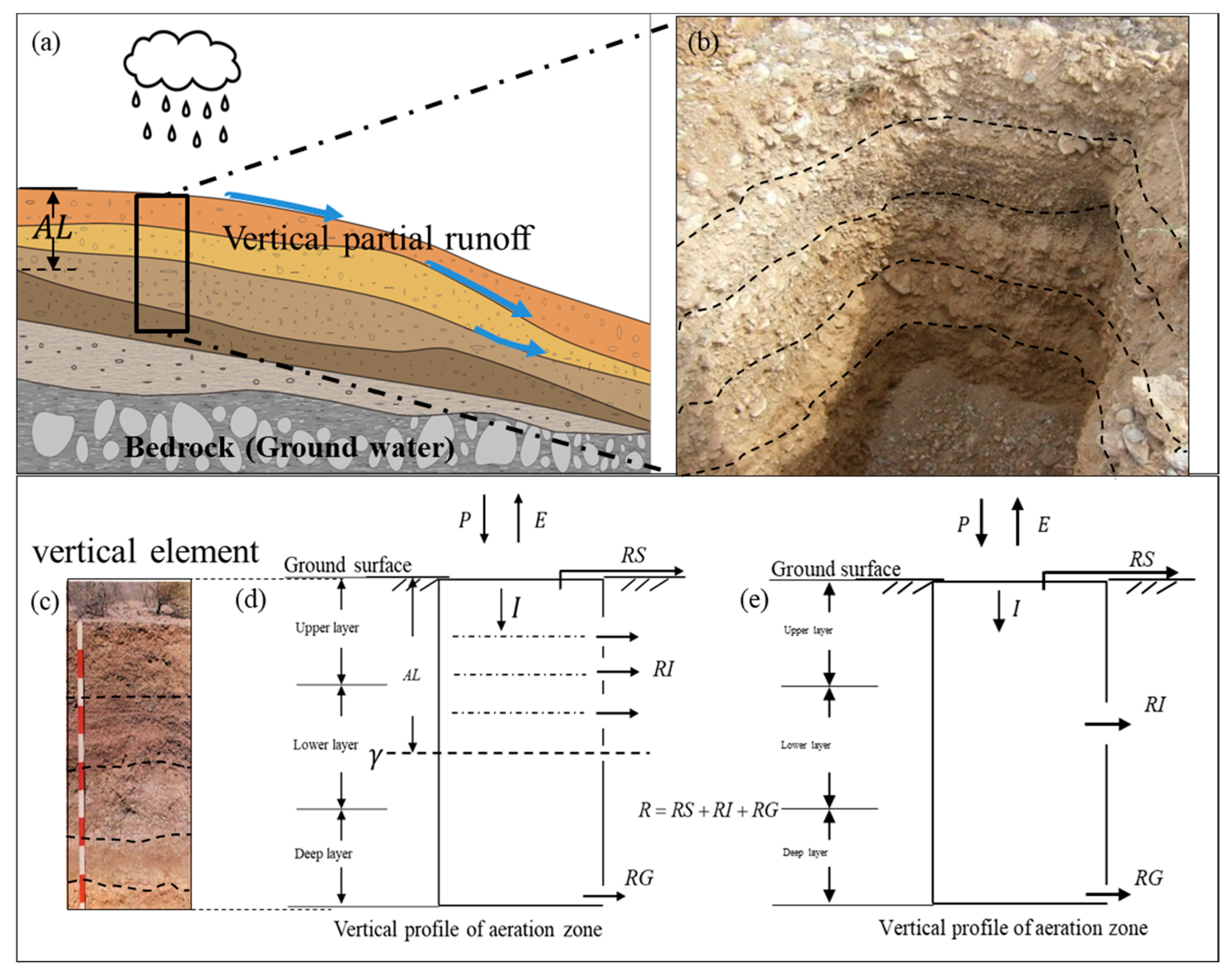
2.1. The Concept of Variable Layer-Based Runoff Generation

The soil in the aeration zone is generally vertically heterogeneous (Figure 1a,b). Relatively impermeable layers generally exist, owing to different infiltration rates of contiguous layers. We drew a conceptual figure to show the generalization of the runoff generation in a hillside and in a vertical element (Figure 1c,d). During rainfall, evapotranspiration (E) was first subtracted and the runoff generation is computed by comparing the soil moisture content and storage capacities in layers. The net rainfall (i.e., P E ) infiltrates downward (denoted as I), the soil content in each layer exceeds the storage capacity of each respective layer successively, and the downward percolation, meanwhile, appears from one layer to another layer. However, the wetting front will stop at a certain depth of the aeration zone, which means that the water content of the whole aeration zone could not easily excess its storage capacity in regions with a large deficiency in soil water storage. The layers over the certain depth can be defined as “active runoff generation layers” (simplified as active layers (AL)), where runoff generates, including surface runoff (RS), interflow (RI), and groundwater runoff (RG). RG will not emerge until γ (ratio of depth of AL to the depth of total aeration zone) reaches the bottom of the aeration zone (i.e., γ = 1 ).
We can thus learn that it is the soil water storage capacity of active layers (AL) that plays a role in controlling the amount of runoff generation (Figure 1d), rather than the storage capacity for total aeration zone used in the XAJ model (Figure 1e). The water storage capacity of active layers (AL) can be defined as relative water storage capacity (RW), which is variable for different rainfall–flood events. Thus, the runoff amount could be estimated if we could identify γ and the corresponding RW for each rainfall–flood event. The runoff generation can be regarded as runoff in excess of partial storage capacity. Compared with the concept of runoff formation on repletion of soil water storage (i.e., the storage–excess concept in XAJ), the concept of runoff in excess of partial storage capacity could simulate the runoff components before the whole aeration zone reaches storage capacity. Whereas for the storage–excess concept in XAJ, runoff is not produced until the soil moisture content of the aeration zone reaches field capacity.

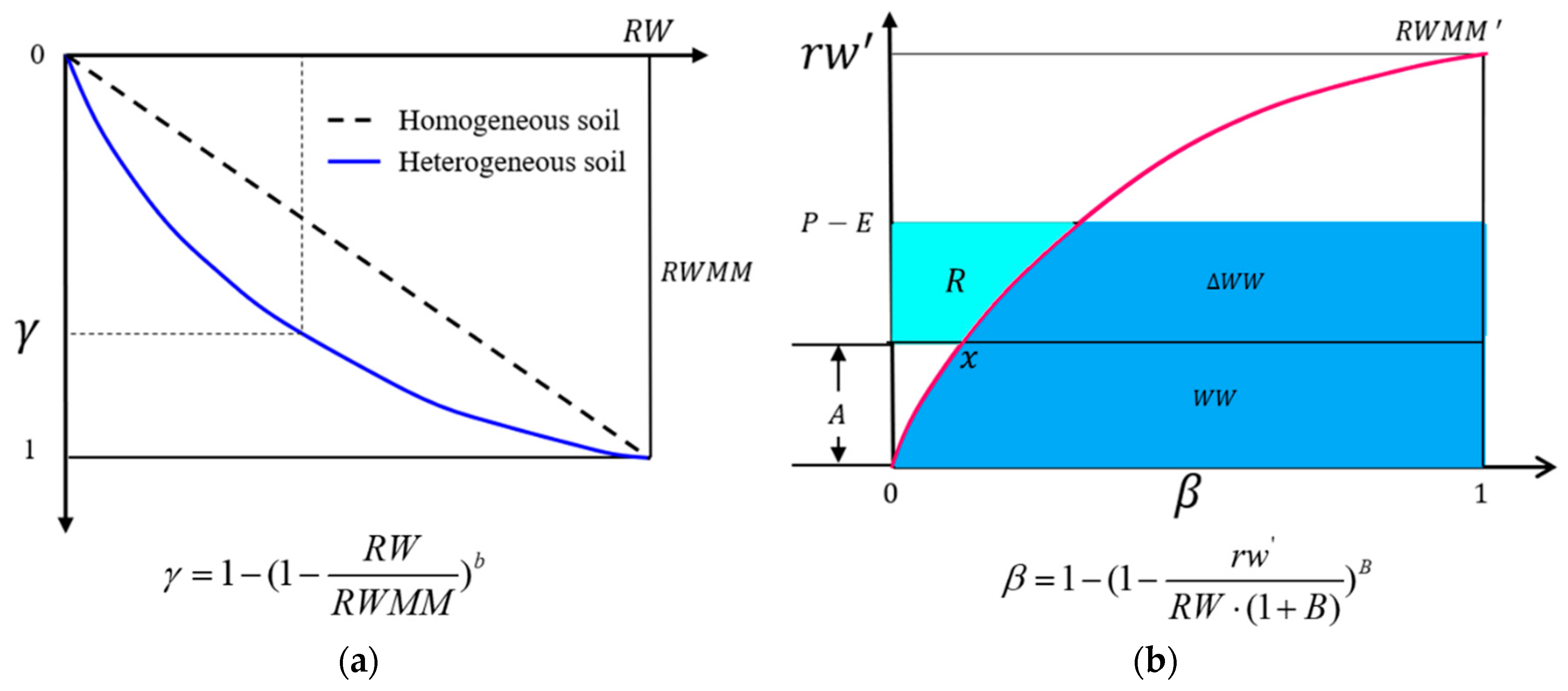
2.2. The Vertical and Spatial Distribution of Relative Water Storage Capacity

2.2.1. The Vertical Distribution

It can be seen in Figure 2a that RW (ranging from 0 to RWMM) is linearly (non-linearly) related to γ for homogeneous (heterogeneous) soil. It is almost impossible to get the vertical distribution of RW for each point of the underlying surface. Here, we try to build the vertical distribution for regional mean RW. The vertical distribution for RW (Figure 2a) can be formulated as:
γ = 1 ( 1 R W R W M M ) b
R W = [ 1 ( 1 γ ) 1 b ] × R W M M
where R W M M denotes the maximum of R W , b is the exponent of the curve which needs to be calibrated in modeling, γ ranges from 0 to 1. The derivations of the equations are shown in Appendix A.
Equation (1) can be used to describe the vertical distribution for the averaged relative water storage capacity over the basin (RW) (Figure 2a). We can learn that it has a similar format to that of the spatial distribution for tension water storage capacity used in the XAJ model. Hence, the parameter b here is also used to adjust the shape of the curve and its value is easy to be established. R W then could be established using Equation (2) given the value of γ during each rainfall–flood event. γ can be regarded as a conceptual state variable that can be obtained through calibration. Generally, the values of γ and RW will be lower during wet phases of soil and larger during dry phases. It depends on the amount of antecedent rainfall and some climate factors.

2.2.2. The Horizontal Spatial Distribution and Runoff Estimation

It should be noted that the RW mentioned above only represents the regional mean of relative soil water storage capacity for a basin (or a sub-basin). It is essential to identify the relative soil water storage capacity at a point (denoted as r w ) over the basin to estimate runoff generation on partial areas.
Runoff production at a point occurs only on repletion of the tension water storage at that point in XAJ model [6]. The concept of using parabolic curve to characterize the spatial distribution for water storage capacity for each point is introduced into this work. We assume that the relative water storage capacity at a point (denoted as r w ) follows the type of spatial distribution used in XAJ model as well (Figure 2b), the spatial distribution of r w can be defined as:
β = 1 ( 1 r w R W M M ) B
where β represents the proportion of the previous area of the basin whose relative water storage capacity is less than or equal to the value of the ordinate r w , B is a parameter. r w varies from 0 to a maximum ( R W M M ).
RW is the areal mean relative water storage capacity, which is the whole area below the curve (Figure 2b). The relation of RW to R W M M can be obtained as follows:
R W = 0 R W M M ( 1 β ) d r w
RW then can be formulated as:
R W = 0 R W M M ( 1 r w R W M M ) B d r w
through integration, we can get R W = R W M M / ( 1 + B ) . Equation (3) therefore can be rewritten as:
β = 1 ( 1 r w R W ( 1 + B ) ) B
Equation (6) describes the spatial distribution curve of relative soil water storage capacity. In Figure 2b, the state of the catchment, at any time, is assumed to be represented by a point x on the curve line. The area to the right and below the point x is proportional to the areal mean relative tension water storage W W (not capacity). This assumption implies that each point in the catchment is either at capacity tension (points to the left of x ) or at a constant tension (points to the right of x ). The area with cyan color (denoted as R) represents the amount of runoff generation. r w is actually a threshold to distinguish whether the runoff is generated or not on a point, and the spatial distribution curve for r w is to control the amount of runoff on partial areas. The runoff process can be deemed as partial storage–excess runoff in A L and on partial areas over the catchment.

2.3. Integration of the Runoff Model into a Hydrological Model

The aforementioned vertical and horizontal distributions for relative water storage capacity are employed to modify the XAJ model, a famous hydrological model widely used in almost all humid and some semi-humid areas in China, so as to improve the efficiency of hydrological simulation and flood forecasts in regions characterized by deficiency in soil water storage, i.e., the semi-humid and semi-arid regions.

2.3.1. Three-Layer Evapotranspiration Module

More details of the three-layer evapotranspiration approach can be referred to Zhao [6]. In this work, the soil moisture in AL (denoted as W W ) at the end of a time step should deduct the corresponding evapotranspiration (E) in AL. The soil moisture content in AL (WW) is approximately estimated by using the following equation based on the relation between R W and R W M M (Equation (2)):
W W = [ 1 ( 1 γ ) 1 b ] × W
where W represents the soil water content of the total aeration zone (i.e., the sum of water content in three-layer soil moisture model). Equation (7) has the advantage of computation convenience. Besides, it is suitable to cooperate with the calculation of conceptual runoff generation. It plays a role to ensure the water balance in AL. The results will be wrong without water balance.

2.3.2. Partial Storage–Excess Runoff Module

When rainfall exceeds evapotranspiration, runoff (R) is generated proportional to the area shown cyan to the left and above the point x in Figure 2b. The calculation of runoff generation includes the following steps.
(1) Step 1: To determine the value of areal mean relative water storage capacity (RW)
RW in each flood event is estimated using the vertical curve represented by Equation (2). Value of γ during each flood is calibrated in modeling.
(2) Step 2: To construct a spatial distribution for relative water storage capacity at a point ( r w )
The spatial distribution curves of r w (Figure 2b) is established according to Equation (6), of which B is uniform during all flood events used for model calibration, owing to that it is an insensitive parameter.
(3) Step 3: To estimate runoff
Case 1: when rainfall exceeds evapotranspiration ( P E > 0 )
If P E + A < R W M M , then
R = P E ( R W W W ) + R W ( 1 P E + A R W ( 1 + B ) ) 1 + B
otherwise,
R = P E ( R W W W )
where A is the ordinate corresponding to soil moisture content (WW) (Figure 2b). Equations (8) and (9) are established through integration of Equation (6) according to Figure 2b. Equations (8) and (9) have the advantage of computation convenience.
Case 2: when evapotranspiration exceeds rainfall ( P E < 0 )
In this case, we deem runoff does not generate. The tension moisture in AL and three tension moisture storages reduce.

2.3.3. Water Source Partition Module

Total runoff R generated on partial areas in accordance with Figure 2b is separated into its two main components, the part emerging on surface (surface runoff ( R S ) and the remaining in subsurface (denoted as R I and R G ) (Figure 1d). R G does not appear until the soil moisture content of the aeration zone at contributing area reaches field capacity. The concept of spatial distribution curve for free water storage capacity is used to separate runoff components (surface runoff ( R S ), interflow ( R I ), and groundwater runoff ( R G )). For more details about separation on runoff components, refer to Zhao [6].

2.3.4. Discharge Routing Module

The hydrodynamic method can be a feasible alternative used for constructing the flow concentration method. In this work, the routing approaches in the XAJ model are directly employed instead of constructing a new method. It helps to ensure that the model developed in this work and the XAJ model have the same flow concentration method, which is for the sake of an impartial comparison between the runoff generation methods. For more details about routing approaches, refer to Zhao [6].

2.4. Measures of Performance Assessment

The following performance measures were used, i.e., the relative error of peak flow (RPF) and runoff depth (RRD), the root mean square error (RMSE) [26], and the Nash–Sutcliffe coefficient (NSE) [27]. RPF was used for evaluating the accuracy of the simulated flow peak and RRD for simulated total runoff depth. NSE and RMSE were used to evaluate the accuracy of simulated hydrograph. In addition, a new model performance criterion termed as the peak percent threshold statistics (PPTS) [28] was employed here to evaluate the performance of the simulation on high flows. RPF, RRD, PPTS, NSE, and RMSE cover almost all the elements that need to be evaluated in flood simulation. These five evaluation criteria collectively show the performance of simulation, which are targeted and comprehensive.
(1) Nash–Sutcliffe efficiency coefficient (NSE)
N S E = 1 j = 1 N [ Q s ( j ) Q o ( j ) ] 2 / j = 1 N [ Q o ( j ) Q o ¯ ] 2
(2) The relative error of peak flow (RPF)
R P F = [ ( Q s p Q o p ) / Q o p ] × 100 %
(3) The relative error of runoff depth (RRD)
R R D = [ ( R s R o ) / R o ] × 100 %
(4) The root mean square error (RMSE)
R M S E = j = 1 N ( Q o ( j ) Q s ( j ) ) 2 N
where Q s is the simulated discharge, Q o is the observed discharge, Q o ¯ is the mean value of observed discharge, N is number of hours in a flood event (the time step in this study is hour), Q s p and Q o p are the simulated and observed peak discharge, respectively, R s is the total runoff depth of the simulated flood event, and R o is the total runoff depth of the observed flood event.
(5) Peak percent threshold statistics (PPTS)
P P T S ( l , u ) = 1 ( k l k u + 1 ) i = k l k u | ξ i |
PPTS is a performance criterion of prediction between top u % and l % data ( P P T S ( l , u ) ). The term is the average absolute relative error in prediction of flows lying in the band of u % and l % data. In which k l = l × N 100 and k u = u × N 100 . Where l and u are lower and higher limits in percentage, respectively, N is the number of data, and ξ i is the average relative error of the i t h data. When the value of u = 100 % , the P P T S ( l , u ) can be represented as P P T S ( l , 100 ) or simply P P T S ( l ) . Further, P P T S ( l ) indicates the peak percent threshold statistics of top l % data [28]. In this work, we use P P T S ( l ) to indicate the peak percent threshold statistics of top l % data. Lower value indicates better performance.

2.5. The Objective Function of Optimization Algorithm

The objective function of the optimization algorithm is shown below. Less value of m u indicates more accurate simulation results. RPF, RRD, and RMSE can be feasible alternative objective functions. Equation (15) is actually the ‘1-NSE’. Compared with other objective functions, it helps to obtain more robust simulation results in terms of lower error and good fitness of streamflow process.
m u = j = 1 N [ Q s ( j ) Q o ( j ) ] 2 j = 1 N [ Q o ( j ) Q o ¯ ] 2
where the meaning of the variables and signs can be referred to the contents above.

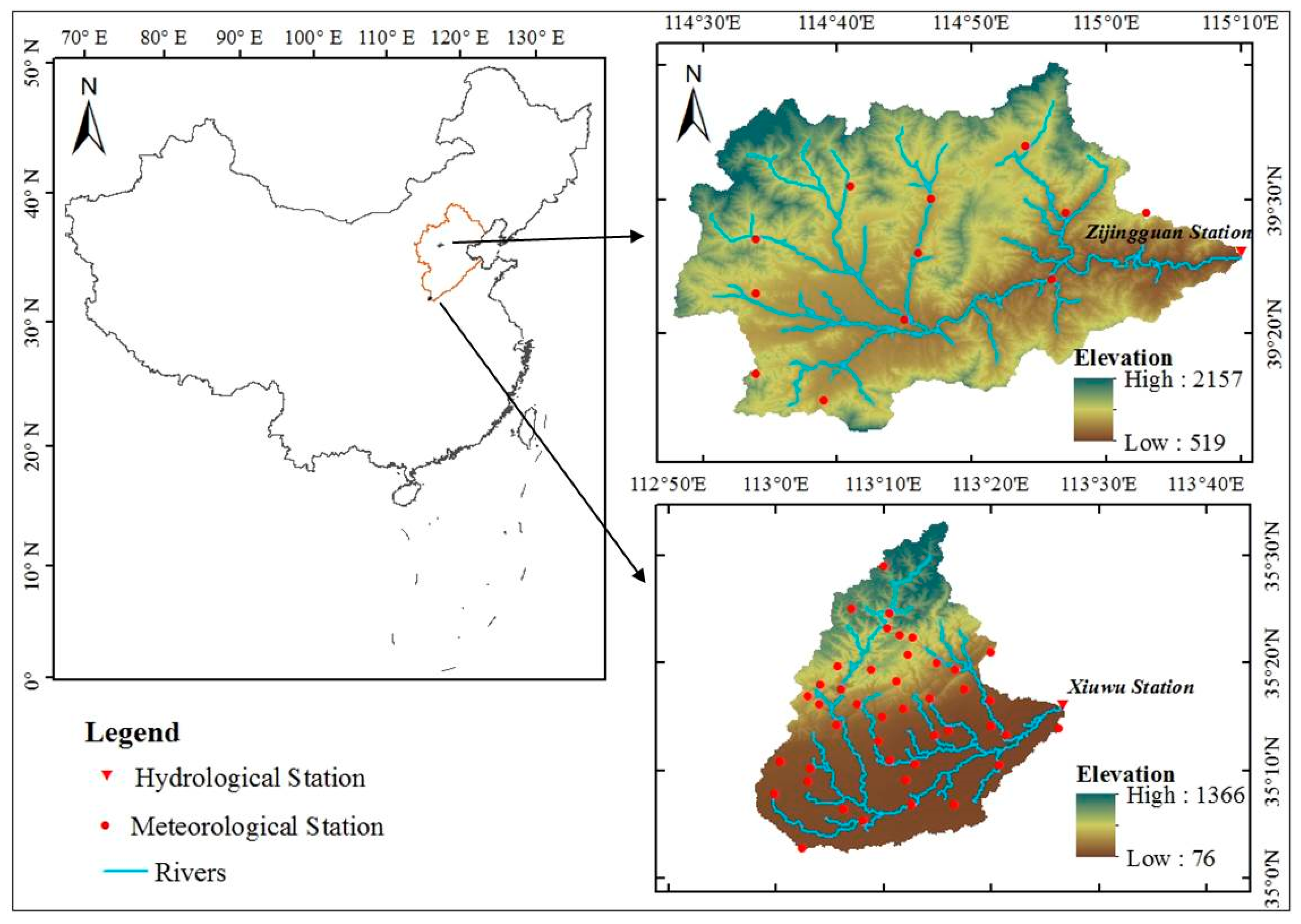
3. Study Area and Data

The runoff model constructed above is a variable layer-based runoff model (denoted as VLRM), which is characterized by the variable runoff layer structure and the concept of runoff formation on repletion of partial storage (partial storage–excess). The ability of the variable runoff layer structure to describe partial runoff and the newly developed VLRM are demonstrated in Haihe River Basin (HRB) (Figure 3), the most typical semi-humid and semi-arid basin in China. Two typical basins (including Zijingguan in the northern part and Xiuwu in the southern part of HRB) were selected to test the model performance.
Zijingguan basin (1760 km2) is located at the northern part of HRB. The elevation ranges from 511 to 2157 m a.s.l. The annual mean precipitation is approximately 543 mm and annual mean temperature is 9.6 °C [29]. Floods in this region are characterized by various hydrographs, including the flashy ones with short time bases and steep rising and falling limbs, and the mild ones with gradual rising and falling during a long time. The basin is in the upriver of Juma River, where a very serious flood happened in July 2012, posing a great threat to Beijing, the capital of China. Xiuwu basin (1287 km2) is located at the southern part of the HRB, the elevation of which ranges from 76 to 1366 m a.s.l. The annual mean precipitation is approximately 608 mm and the annual mean air temperature is 14 °C. More than 50% of the total annual precipitation happens in July and August, and a lot of flood events occur over this basin. The runoff coefficients are small in these two basins. The runoff coefficients in Zijingguan basin range from 0.04 to 0.42, most of which concentrate in the interval 0.04–0.25. The runoff coefficients in Xiuwu basin range from 0.05 to 0.23. The low runoff coefficients indicate great water deficiency of soil water content. Data are compiled from several historical flood events, including the hourly precipitation, hourly flow data, and daily observed evaporation by evaporator. The latter is interpolated into hourly data.

4. Results

4.1. Optimised Parameter Values

Model calibration and verification were carried out using hourly flood event data. For Zijingguan basin, 15 middle and large flood events were collected, of which nine were for calibration and six were for validation. For Xiuwu basin, 30 middle and large flood events were collected, of which 20 were for calibration and 10 were for validation. They are middle and large floods, which are of great concern to the government and hydrologists. The simulation and forecast of these flood events is a difficulty nowadays. A successful simulation on these flood events could demonstrate the performance of the proposed model.
The γ in partial storage–excess runoff module in each flood and the model parameters are optimally calibrated using the shuffled complex evolution method (SCE-UA) [30,31,32]. Feasible alternatives include the Gauss–Newton algorithm [31], surrogate models [33], and genetic algorithms [34], etc., SCE-UA does not rely on gradients and hence is largely insensitive to micro-scale roughness, while the stochastic nature helps to avoid entrapment in local optima. The favorable global convergence properties have been established empirically over many case studies [35,36]. W U , W L , and W D are the soil moisture contents of the upper layer, lower layer, and deep layer of soil at the initial time of each flood event, respectively. In a real-time flood forecasting, these initial conditions are commonly assigned values based on the continuous running results [6]. In this work for simulation, they are pre-set and adjusted during the warm-up period.

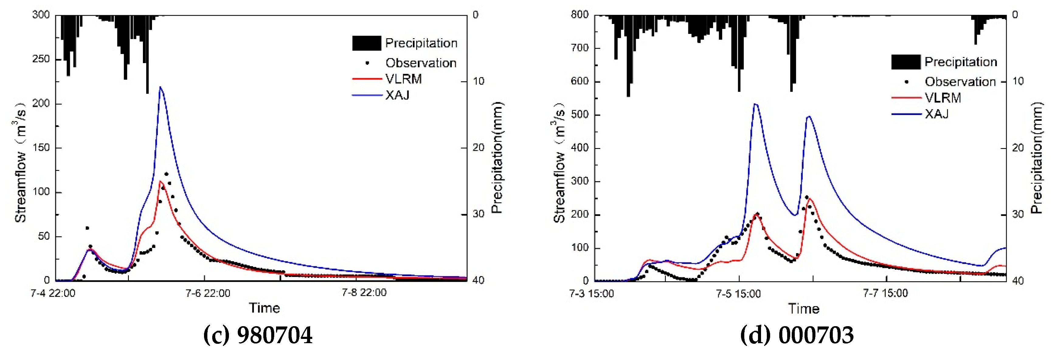
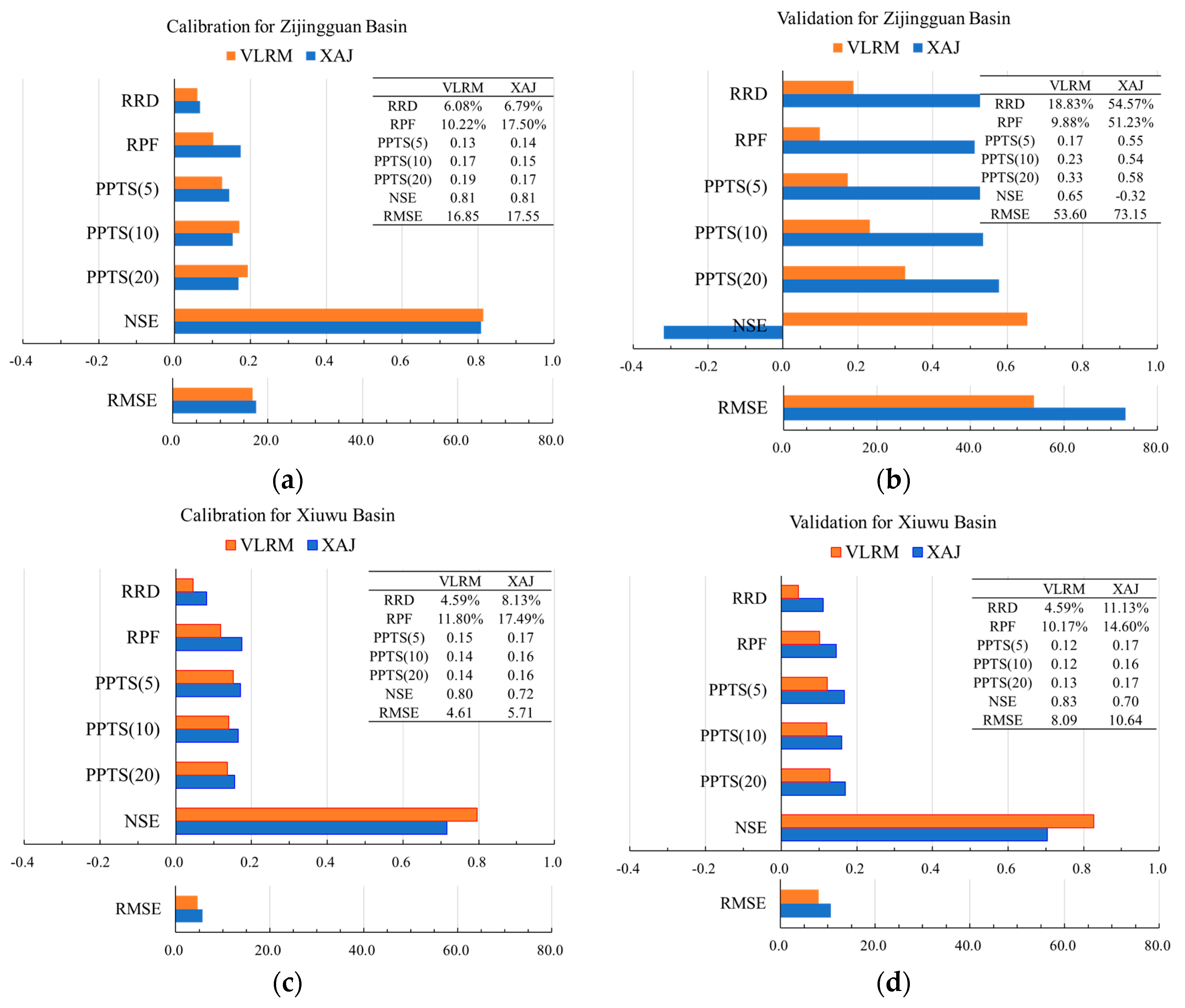
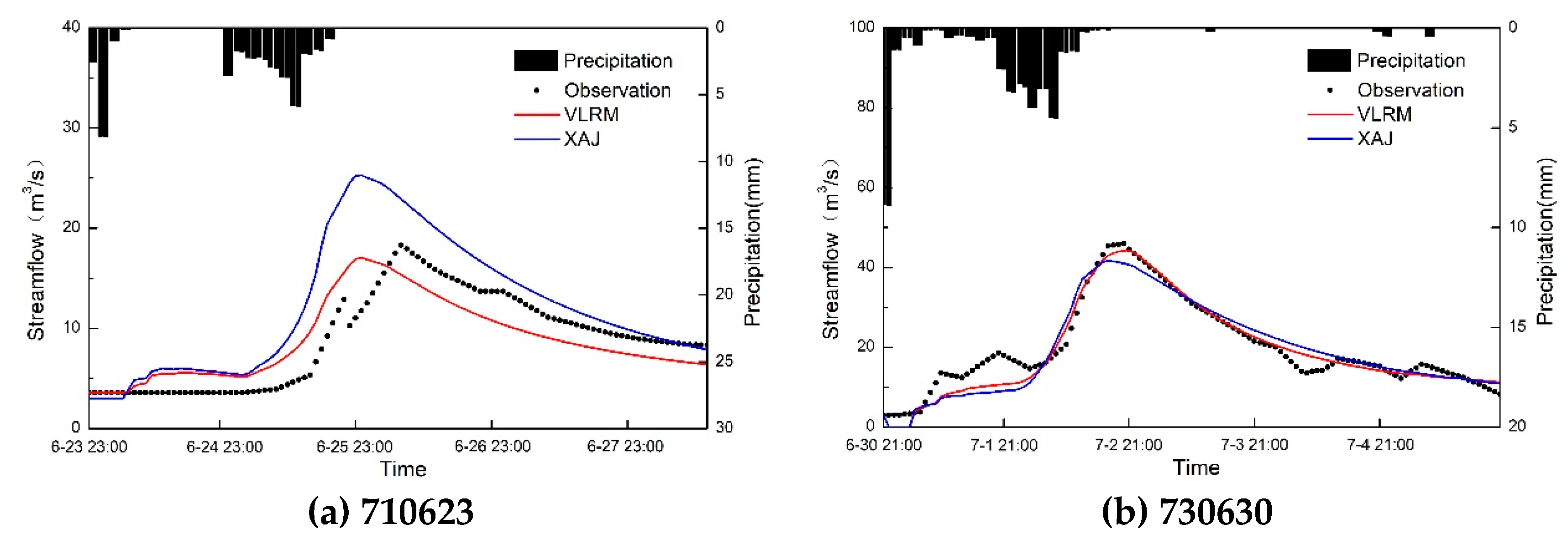
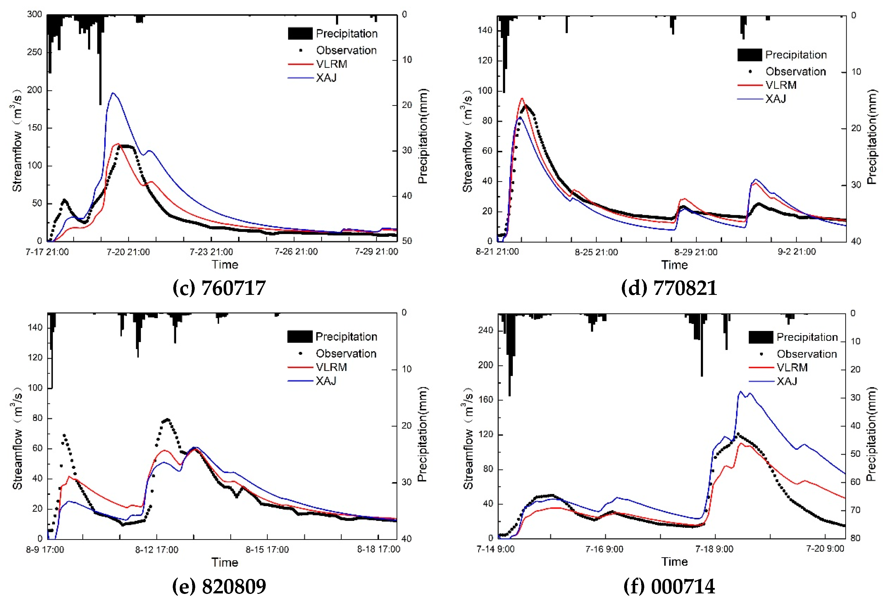
4.2. Statistical and Graphic Presentation of the Results

The calibrated model parameters of VLRM are shown in Table 1. The XAJ model [6] is employed here to conduct a comparison with VLRM. It is difficult to demonstrate the performance of the modified runoff method through a comparison with other hydrological models, as models have different structures. The difference in efficiency amongst the approaches for evapotranspiration, infiltration, and flow routing will confuse the comparison. The performance improvement induced by modified runoff method could not be separated and identified. Therefore, only the original XAJ model was selected to make a comparison with VLRM.
Table 2 shows the comparison of performance measures for the simulation by VLRM and XAJ model, and Figure 4 shows the hydrographs of typical flood events in both calibration and validation periods in Zijingguan basin. To clearly show the performance measures and better compare the performance of the two models, the average values of each measure for all flood events are aggregated in Figure 5. In the calibration period (Figure 5a), the average RRD is 6.08% by VLRM and 6.79% by XAJ. The average RPF by VLRM and XAJ are 10.22% and 17.50%, respectively. Lower RRD and RPF indicate that VLRM has a better simulation for total runoff depth and peak flow. On the other hand, the PPTS (5) by VLRM is lower than that by XAJ, whereas the PPTS (10) and PPTS (20) by VLRM are little higher than that by XAJ. What is more, the average NSE by VLRM and XAJ is almost the same, and RMSE by VLRM is better than that by XAJ. In short, VLRM performs a little better than XAJ in the calibration period, though not all statistical measures by VLRM show better values. The advantage is not significant (e.g., Figure 4a,b).
On the contrary, the difference of each performance measure by VLRM and XAJ are obvious in the validation period (Figure 5b and Figure 4c–d). The VLRM shows significantly better performance than XAJ. The average RRD is 18.83% by VLRM and 54.57% by XAJ, and the average RPF is 9.88% by VLRM and 51.23% by XAJ, together showing a better performance of VLRM on simulation total runoff depth and peak flow. In addition, the PPTS statistics by VLRM are both lower than that by XAJ, indicating a better simulation on high flows by VLRM. What is more, the average NSE and RMSE consistently show that VLRM better captures the changing behaviors of flood hydrograph (Figure 4c,d). The NSE for each flood event by VLRM in the validation period are both beyond 0.70, except one event (950722) (Table 2). Whereas, three flood events (950722, 980704, and 000703) by XAJ are not qualified (Table 2).
Table 3 shows the comparison of performance measures for the simulation by the VLRM and XAJ models, and Figure 6 shows the hydrographs of typical flood events in both calibration and validation periods for Xiuwu basin. Figure 5c–d shows the average values of each measure for all flood events. It is seen that VLRM outperforms XAJ in all statistical measures in the calibration period (Figure 5c). The average RRD is 4.59% by VLRM and 8.13% by XAJ. The average RPF by VLRM and XAJ are 11.80% and 17.49%, respectively. Lower RRD and RPF indicate that VLRM has a better simulation on total runoff depth and peak flow, respectively. On the other hand, the PPTS measures (PPTS (5), PPTS (10), and PPTS (20)) indicate a better simulation on high flow by VLRM, which is quite important for flood simulation and forecast. The average NSE by VLRM and XAJ are 0.80 and 0.72, respectively. The average RMSE by VLRM and XAJ are 4.61 and 5.71, respectively. Higher NSE and lower RMSE indicate that VLRM makes a better simulation on flood hydrograph than XAJ does. In the validation period, the VLRM has a better performance than XAJ as well (Figure 5d). It can be concluded that the VLRM outperforms XAJ both in calibration and validation periods in Xiuwu basin.

4.3. Sensitivity and Uncertainty Analyses

The VLRM is developed based on XAJ model through adding a variable runoff generation layer in terms of the vertical distribution of relative water storage capacity. Other parts of the model are not changed. Hence, it is likely that the better performance of VLRM over XAJ can be attributed to the improvement on runoff estimation method in terms of the additional vertical distribution of relative water storage capacity. The parameter b, RWMM, and state variable γ constitute the vertical distribution for the averaged relative water storage capacity over the basin (Equation (1)). The Markov chain Monte Carlo (MCMC) method [37], the Latin hypercube one factor at a time (LH-OAT) method [38], and the generalized likelihood uncertainty estimation (GLUE) [39] approach can be used to conduct sensitivity and uncertainty analysis on parameters. In this work, GLUE is employed to conduct brief sensitivity and uncertainty analysis on parameters b and RWMM to reveal their characteristics and the effect on hydrograph. The GLUE approach shows the following advantages: (1) it is logically simple with no strict error assumptions [37], and (2) it is insensitive to the discontinuous parameter surface of complex hydrological models characterized by dozens of parameters [40].
The Nash–Sutcliffe efficiency coefficient (NSE) is used as an indicator to describe the response of hydrograph to the changes in parameters (Figure 7). For Zijingguan basin, the RWMM is given an interval around the optimal value of RWMM (Figure 7a), and all the other parameters are given intervals according to Table 1. It is seen that NSE is sensitive to the value of RWMM. When RWMM is less than 400, NSE is difficult to exceed 0.70. On the other hand, parameter b is not sensitive given the value interval 1.0–1.5 (Figure 7b). For Xiuwu basin, RWMM is sensitive as well (Figure 7c). When RWMM is less than 370, NSE is difficult to exceed 0.60. The parameter b is not sensitive (Figure 7d), which is similar to that for Zijingguan basin. In short, b is not sensitive and RWMM is lightly sensitive. γ and the corresponding RW actually play a role in providing a variable threshold for runoff generation for each flood event.

5. Discussion

The parameter RWMM in VLRM is consistent with the parameter WM in XAJ in that they have a similar physical significance. Only the parameter b is a new additional parameter used in the vertical distribution for relative soil water storage capacity. The ratio of the impervious to total area of the basin (IM) used in XAJ is not used in VLRM. Hence, the number of parameters in VLRM is the same of that in XAJ. The improvement on runoff model through adding the vertical distribution for relative water storage capacity does not increase the number of parameters. Additionally, only the runoff generation method was improved and the other parts of the model were not changed. Therefore, the improvement of performance should be attributed to the concept of variable soil water storage capacity and the description of partial runoff in the variable active layer.
It is known that floods in regions characterized by deficiency in soil water storage are difficult to simulate and forecast. These regions are often in a delicate hydrological balance. The whole nature of the hydrology and, hence, the values of model parameters may be changed by a prolonged wet or dry sequence [25]. A prolonged wet condition may make the hydrological process similar to that in humid regions, whereas a prolonged dry condition makes it similar to that in arid regions. This delicate hydrological balance poses a great challenge for hydrological modeling (especially for flood forecasting) [41], calling for a great effort to construct a new runoff pattern.
The infiltration capacity is highly influenced by the variable rainfall (intensity and amount) and soil moisture content, introducing large difficulties and uncertainties into simulating the runoff and streamflow [42,43], which may be one of the key reasons for the poor performance of excess-infiltration based models [21,25,44]. In addition, the widely used concept of runoff formation on repletion of aeration zone storage cannot be employed to successfully describe the runoff generation process in the dry area as well [6,21,44]. It has been proved by previous studies that the storage–excess based models are not suitable for the semi-arid and arid regions [24]. It is mainly because that the precipitation, runoff generation, and soil moisture in these regions have large spatial and temporal heterogeneities [45]. The appreciable recharge of aquifers from general infiltration sometimes occurs only in extreme events in most semi-arid regions and some semi-humid regions with low underground water levels [25,46], that is to say, the infiltration wetting front generally reaches shallow depths and hereby the storage of aeration zone tends not to be fulfilled during one or more rainfall events.
In this paper, the new concept of active runoff generation layers and runoff formation on repletion of partial storage actually provides a variable threshold to distinguish the generation of runoff. The relative soil water storage capacity is variable during different floods, the concept of runoff generation in active layers therefore is not succumbed to the delicate hydrological balance (i.e., a prolonged wet or dry condition). It plays a consistent role in charactering and estimating the runoff process in semi-humid and semi-arid regions. It is the reason why VLRM performs well in the validation period for Zijingguan basin (Table 2, Figure 4c,d, and Figure 5b). The diverse runoff coefficients (ranging from 0.04 to 0.42) in Zijingguan basin indicates a complicated runoff generation process resulting from variable rainfall and soil moisture content [21]. The annual streamflow of Zijingguan basin decreases significantly because of the impact of human activity (e.g., over extraction of groundwater) and climate change after the 1990s [47,48,49], leading to great changes in runoff generation conditions and flow regimes [50,51,52,53]. In some dry periods, the river even runs out of discharge. Whereas, the basin sometimes suffers flood triggered by heavy storms as well. The runoff concept of storage–excess could not simulate the complex runoff process when the soil could not be saturated. It is the reason why the XAJ model performs poorly in the validation period (Figure 6b, Table 2).
The advisement for the value interval of parameters is shown in Table 1. The value intervals of some parameters related to soil moisture (UM and LM) are defined according to their significance. In dry regions, the intervals of UM and LM in Table 1 are feasible. In humid or wet regions, the upper limit of the intervals should be lower (100 is suited). On the other hand, the ranges of the special parameters (RWMM and b) in VLRM are established according to their significance together with the results of sensitivity analysis (Figure 7). RWMM should be lower (150–300) when applying the model in humid basins. The parameters KC, C, B, SM, EX, KI, KG, CS, CI, CG, KE, and XE are the same as those in the XAJ model, the domains of which can be referred to by Zhao [6].
The model implicitly considers the influence of vegetation and land use in terms of model structure and parameters. In VLRM, the influence of vegetation is considered in terms of parameters UM, C, and SM. UM is the tension moisture capacity of the upper layer, which includes vegetation interception. C is the coefficient of deep evapotranspiration, which depends on the area of deep root plants. SM is related to the density of vegetation. SM is large in dense forest. On the other hand, the spatial distribution curves for relative water storage capacity and free water storage capacity, and the corresponding parameters RWMM, B, SM, and EX, collectively represent the spatially different storage capacity due to diverse land use.
Though previous similar studies investigated the streamflow prediction [42], the impact of climate change and human activities on the hydrological process [46,48,49], and the flow regime alteration under changing environment [50,51,52,53], few of them focus on the partial runoff process and runoff pattern. This study concentrates on the identification of complex partial runoff and the estimation of runoff generation. The variable threshold for runoff generation, the new runoff concept based on active layers, and the new model collectively constitute the distinctive deliverables to provide beneficial insights in developing more robust hydrological modelling approaches in regions characterized by deficiency in soil water storage.

6. Conclusions

In this paper, the vertical partial runoff issue commonly existing in regions with a large deficiency in soil water storage are characterized. A new concept of runoff generation on repletion of partial storage is proposed to describe the vertical partial runoff. The vertical and horizontal distribution curves for relative soil water storage capacity are constructed to characterize the non-uniformity of the soil water deficiency over the catchment. The concept of runoff generation and the approaches for partial runoff estimation collectively constitute the distinctive deliverables to provide beneficial insights in understanding the intricate and distinct behaviors of the rainfall-runoff process, and simulating and forecasting flood in regions characterized by deficiency in soil water storage.
The concept of runoff generation on repletion of partial storage in the active layers and the corresponding approaches for partial runoff estimation are integrated into a rainfall–runoff model (denoted as VLRM). The application of VLRM in two case studies conducted in Haihe River Basin demonstrate that the runoff theory and approaches in this article perform well in simulating various kinds of floods. A series of measures for performance evaluation (i.e., RRD, RPF, NSE, RMSE, and PPTS) collectively show that the VLRM model outperforms the XAJ model in flood simulation, which may be the powerful evidence for the reasonability of the vertical partial runoff theory and approaches. In addition, the sensitivity analysis on the additional parameters indicate that the improvement of the performance should be attributed to the concept of variable soil water storage capacity and the description of partial runoff in the variable active layer. What is more, the improvement on the runoff model through adding the vertical distribution for relative water storage capacity does not increase the number of parameters, which is the same as that of XAJ. The technique can be widely used to simulate and forecast floods in other similar regions. The symbols and the definitions of the variables used in the paper are shown in Table A1 of Appendix B.
The identification of the depths of runoff generation active layers and the corresponding water deficiency or storage capacity need to be further investigated in our further research. The type of distribution of relative storage capacity needs to be further improved through numerical and in-situ physical observation experiments. In detail, the assumption of different relations between φ ( R W ) and [ 1 F ( R W ) ] (shown in Appendix A) will lead to different equations for RW and diverse model efficiency. The evaluation of the model efficiency based on different equations and the influence from assumption will be further investigated in our future study. On the other hand, the forecasting of river systems and its water flow behaviors is particularly difficult, owing to the complex physical process and natural variabilities, posing a great challenge to the conventional methods. The physical models integrated with the artificial intelligence (AI) approaches [54,55,56] should be further investigated in future studies. The AI methods can help to describe the complex non-linear relations existing in the hydrological process, which could not be well characterized by the current conventional methods.

Author Contributions

Conceptualization, P.S. and T.Y.; methodology, P.S., Z.L., and B.Y.; software, P.S., Z.L.; validation, T.Y., C.-Y.X.; formal analysis, Z.L., X.W., and Y.Q.; investigation, X.Z. and S.L.; resources, T.Y.; data curation, Z.L.; Writing—Original draft preparation, P.S.; Writing—Review and editing, P.S., C.-S.H.; visualization, X.W.; supervision, T.Y. and C.-Y.X.; project administration, P.S.; funding acquisition, P.S. and T.Y.

Funding

This research was funded by grants from the National Natural Science Foundation of China (51809072, 51879068), a grant from the Fundamental Research Funds for the Central Universities (2019B16914), a grant from Key R&D Program of Ningxia (20175046802), and a grant from National Key R&D Program of China (2018YFC0407900).

Acknowledgments

Authors are thankful to Hohai University for giving space and funding to carry out the research work. All the authors are highly thankful to the reviewers for their fruitful comments to improve the quality of the paper.

Conflicts of Interest

The authors declare no conflict of interest. The funders had no role in the design of the study; in the collection, analyses, or interpretation of data; in the writing of the manuscript, or in the decision to publish the results.

Appendix A

To establish the formula for vertical distribution of regional mean RW, we deduce the relationship between γ and RW as follows.
RW is expected to increase with the increase of γ , the function hence can be formulated as:
γ = F ( R W )
the differential function for F ( R W ) then can be obtained:
φ ( R W ) = d F ( R W ) d R W
accordingly, F ( R W ) or γ can be expressed as the form of integral function for φ ( R W ) :
F ( R W ) = 0 R W φ ( R W ) d R W
F ( R W M M ) = 0 R W M M φ ( R W ) d R W = 1
to derive the definite functions for F ( R W ) and φ ( R W ) , a simple and practical way is to assume that φ ( R W ) is in direct proportion to [ 1 F ( R W ) ] :
φ ( R W ) = k [ 1 F ( R W ) ]
d F ( R W ) = k [ 1 F ( R W ) ] d R W
F ( R W ) therefore could be obtained in the form that follows through integration:
F ( R W ) = 1 e k R W C
F ( R W ) = 1 D e k R W
φ ( R W ) = k D e k R W
where C is a constant term, D = e C , and k > 0. According to Equation (8) and the definition of γ and RW, we can know that γ or F ( R W ) is 0 when RW is 0. It then can be known that D = 1 and Equation (8) can be formulated as:
γ = 1 e k R W
the interval of k value could not be easily obtained, restricting the model calibration. Hence, we reform it according to Taylor’s theorem as follows. An exponential function e d R W could be written as the form of Taylor expansion:
e d R W = 1 + d R W 1 ! + d 2 R W 2 2 ! + d 3 R W 3 3 ! +
where d is a constant. Take its first order approximation:
e d R W = 1 + d R W 1 !
e k R W = ( e d R W ) k d = ( 1 d R W ) k d
Equation (10) then can be reformulated as:
γ = 1 ( 1 d R W ) k d
we can know that γ or F ( R W ) is 1 when RW take the maximum value RWMM (i.e., the regional averaged soil water storage capacity for the total thickness of aeration zone) according to the definition of γ and RW:
1 = 1 ( 1 d R W M M ) k d
we can therefore obtain d = 1 / R W M M , and Equation (14) can be rewritten as:
γ = 1 ( 1 R W R W M M ) k R W M M
for a certain basin, RWMM is a fixed value. Let b = k R W M M , Equation (16) can be formulated as:
γ = 1 ( 1 R W R W M M ) b
R W = [ 1 ( 1 γ ) 1 b ] × R W M M
where R W M M denotes the maximum of R W , b is the exponent of the curve which needs to be calibrated in modeling, γ ranges from 0 to 1.

Appendix B

Table A1. The symbols and the definitions of the variables used in the paper.
VariablesDescription
ParametersKCRatio of potential evapotranspiration to pan evaporation
UMTension moisture capacity of upper layer
LMTension moisture capacity of lower layer
CCoefficient of deep evapotranspiration
RWMMThe averaged soil water storage capacity for the whole aeration zone
bExponent of the vertical distribution curve for relative water storage capacity
BExponent of the spatial distribution curve for relative water storage capacity
SMAverage free water storage capacity
EXExponent of the free water storage capacity curve
KIOutflow coefficient of the free water storage to interflow
KGOutflow coefficient of the free water storage to groundwater
CSRecession constant of the surface water
CIRecession constant of the lower interflow storage
CGRecession constant of the groundwater storage
KEParameter of Muskingum routing
XEParameter of Muskingum routing
Conceptual state variables γ ratio of depth of AL to the depth of total aeration zone
WUSoil moisture content of upper layer
WLSoil moisture content of upper layer
WDSoil moisture content of upper layer
WWSoil moisture content in AL
Δ W W Changes of WW
Symbols in the figuresALActive runoff generation layers
PPrecipitation
EEvapotranspiration
RRunoff
RSSurface runoff
RIInterflow
RGGroundwater runoff
RWRelative water storage capacity
β The proportion of the runoff area to the basin
Performance measuresRPFThe relative error of peak flow
RRDThe relative error of runoff depth
RMSEThe root mean square error
NSEThe Nash–Sutcliffe coefficient
PPTSThe peak percent threshold statistics

References

  1. Chuntian, C.; Chau, K.W. Three-person multi-objective conflict decision in reservoir flood control. Eur. J. Oper. Res. 2002, 142, 625–631. [Google Scholar] [CrossRef] [Green Version]
  2. Cloke, H.L.; Pappenberger, F. Ensemble flood forecasting: A review. J. Hydrol. 2009, 375, 613–626. [Google Scholar] [CrossRef]
  3. Moore, R.J.; Bell, V.A.; Jones, D.A. Forecasting for flood warning. C. R. Geosci. 2005, 337, 203–217. [Google Scholar] [CrossRef]
  4. Yaseen, Z.M.; Sulaiman, S.O.; Deo, R.C.; Chau, K.-W. An enhanced extreme learning machine model for river flow forecasting: State-of-the-art, practical applications in water resource engineering area and future research direction. J. Hydrol. 2019, 569, 387–408. [Google Scholar] [CrossRef]
  5. Ameli, A.A.; Craig, J.R.; McDonnell, J.J. Are all runoff processes the same? Numerical experiments comparing a Darcy-Richards solver to an overland flow-based approach for subsurface storm runoff simulation. Water Resour. Res. 2015, 51, 10008–10028. [Google Scholar] [CrossRef] [Green Version]
  6. Zhao, R.-J. The Xinanjiang model applied in China. J. Hydrol. 1992, 135, 371–381. [Google Scholar] [CrossRef]
  7. Beven, K. Towards an alternative blueprint for a physically based digitally simulated hydrologic response modelling system. Hydrol. Process. 2002, 16, 189–206. [Google Scholar] [CrossRef] [Green Version]
  8. Liang, X.; Lettenmaier, D.P.; Wood, E.F. One-dimensional statistical dynamic representation of subgrid spatial variability of precipitation in the two-layer variable infiltration capacity model. J. Geophys. Res. Atmos. 1996, 101, 21403–21422. [Google Scholar] [CrossRef]
  9. Devia, G.K.; Ganasri, B.P.; Dwarakish, G.S. A Review on Hydrological Models. Aquat. Procedia 2015, 4, 1001–1007. [Google Scholar] [CrossRef]
  10. Hao, G.; Li, J.; Song, L.; Li, H.; Li, Z. Comparison between the TOPMODEL and the Xin’anjiang model and their application to rainfall runoff simulation in semi-humid regions. Environ. Earth Sci. 2018, 77, 279. [Google Scholar] [CrossRef]
  11. Chawla, I.; Mujumdar, P.P. Partitioning uncertainty in streamflow projections under nonstationary model conditions. Adv. Water Resour. 2018, 112, 266–282. [Google Scholar] [CrossRef]
  12. Raju, B.C.K.; Nandagiri, L. Assessment of variable source area hydrological models in humid tropical watersheds. Int. J. River Basin Manag. 2018, 16, 145–156. [Google Scholar] [CrossRef]
  13. Golmohammadi, G.; Rudra, R.; Dickinson, T.; Goel, P.; Veliz, M. Predicting the temporal variation of flow contributing areas using SWAT. J. Hydrol. 2017, 547, 375–386. [Google Scholar] [CrossRef]
  14. Kim, S.J.; Steenhuis, T.S. Gristorm: Grid–Based Variable Source Area Storm Runoff Model. Trans. ASAE 2001, 44, 863. [Google Scholar] [CrossRef]
  15. Ivanov, V.Y.; Vivoni, E.R.; Bras, R.L.; Entekhabi, D. Catchment hydrologic response with a fully distributed triangulated irregular network model. Water Resour. Res. 2004, 40. [Google Scholar] [CrossRef]
  16. Daneshmand, H.; Alaghmand, S.; Camporese, M.; Talei, A.; Daly, E. Water and salt balance modelling of intermittent catchments using a physically-based integrated model. J. Hydrol. 2019, 568, 1017–1030. [Google Scholar] [CrossRef]
  17. Schneiderman, E.M.; Steenhuis, T.S.; Thongs, D.J.; Easton, Z.M.; Zion, M.S.; Neal, A.L.; Mendoza, G.F.; Todd Walter, M. Incorporating variable source area hydrology into a curve-number-based watershed model. Hydrol. Process. 2007, 21, 3420–3430. [Google Scholar] [CrossRef]
  18. Dahlke, H.E.; Easton, Z.M.; Fuka, D.R.; Lyon, S.W.; Steenhuis, T.S. Modelling variable source area dynamics in a CEAP watershed. Ecohydrology 2009, 2, 337–349. [Google Scholar] [CrossRef]
  19. Lee, K.T.; Huang, J.-K. Runoff simulation considering time-varying partial contributing area based on current precipitation index. J. Hydrol. 2013, 486, 443–454. [Google Scholar] [CrossRef]
  20. Cantón, Y.; Rodríguez-Caballero, E.; Chamizo, S.; Le Bouteiller, C.; Solé-Benet, A.; Calvo-Cases, A. Chapter 5—Runoff Generation in Badlands. In Badlands Dynamics in a Context of Global Change; Nadal-Romero, E., Martínez-Murillo, J.F., Kuhn, N.J., Eds.; Elsevier: Amsterdam, The Netherlands, 2018; pp. 155–190. [Google Scholar]
  21. Huang, P.; Li, Z.; Chen, J.; Li, Q.; Yao, C. Event-based hydrological modeling for detecting dominant hydrological process and suitable model strategy for semi-arid catchments. J. Hydrol. 2016, 542, 292–303. [Google Scholar] [CrossRef]
  22. Dunne, T.; Black, R.D. Partial Area Contributions to Storm Runoff in a Small New England Watershed. Water Resour. Res. 1970, 6, 1296–1311. [Google Scholar] [CrossRef] [Green Version]
  23. Daliakopoulos, I.N.; Tsanis, I.K. Comparison of an artificial neural network and a conceptual rainfall–runoff model in the simulation of ephemeral streamflow. Hydrol. Sci. J. 2016, 61, 2763–2774. [Google Scholar] [CrossRef]
  24. Jayawardena, A.W.; Zhou, M.C. A modified spatial soil moisture storage capacity distribution curve for the Xinanjiang model. J. Hydrol. 2000, 227, 93–113. [Google Scholar] [CrossRef]
  25. Pilgrim, D.H.; Chapman, T.G.; Doran, D.G. Problems of rainfall-runoff modelling in arid and semiarid regions. Hydrol. Sci. J. 1988, 33, 379–400. [Google Scholar] [CrossRef]
  26. Moazenzadeh, R.; Mohammadi, B.; Shamshirband, S.; Chau, K.-W. Coupling a firefly algorithm with support vector regression to predict evaporation in northern Iran. Eng. Appl. Comput. Fluid Mech. 2018, 12, 584–597. [Google Scholar] [CrossRef] [Green Version]
  27. Si, W.; Bao, W.; Gupta, H.V. Updating real-time flood forecasts via the dynamic system response curve method. Water Resour. Res. 2015, 51, 5128–5144. [Google Scholar] [CrossRef]
  28. Lohani, A.K.; Goel, N.K.; Bhatia, K.K.S. Improving real time flood forecasting using fuzzy inference system. J. Hydrol. 2014, 509, 25–41. [Google Scholar] [CrossRef]
  29. Li, J.; Feng, P.; Chen, F. Effects of land use change on flood characteristics in mountainous area of Daqinghe watershed, China. Nat. Hazards 2014, 70, 593–607. [Google Scholar] [CrossRef]
  30. Duan, Q.Y.; Gupta, V.K.; Sorooshian, S. Shuffled complex evolution approach for effective and efficient global minimization. J. Optim. Theory Appl. 1993, 76, 501–521. [Google Scholar] [CrossRef]
  31. Qin, Y.; Kavetski, D.; Kuczera, G. A Robust Gauss-Newton Algorithm for the Optimization of Hydrological Models: From Standard Gauss-Newton to Robust Gauss-Newton. Water Resour. Res. 2018, 54, 9655–9683. [Google Scholar] [CrossRef]
  32. Qin, Y.; Kavetski, D.; Kuczera, G. A Robust Gauss-Newton Algorithm for the Optimization of Hydrological Models: Benchmarking Against Industry-Standard Algorithms. Water Resour. Res. 2018, 54, 9637–9654. [Google Scholar] [CrossRef]
  33. Queipo, N.V.; Haftka, R.T.; Shyy, W.; Goel, T.; Vaidyanathan, R.; Kevin Tucker, P. Surrogate-based analysis and optimization. Prog. Aerosp. Sci. 2005, 41, 1–28. [Google Scholar] [CrossRef] [Green Version]
  34. Wang, Q.J. The Genetic Algorithm and Its Application to Calibrating Conceptual Rainfall-Runoff Models. Water Resour. Res. 1991, 27, 2467–2471. [Google Scholar] [CrossRef]
  35. Duan, Q.; Sorooshian, S.; Gupta, V. Effective and efficient global optimization for conceptual rainfall-runoff models. Water Resour. Res. 1992, 28, 1015–1031. [Google Scholar] [CrossRef]
  36. Tolson, B.A.; Shoemaker, C.A. Dynamically dimensioned search algorithm for computationally efficient watershed model calibration. Water Resour. Res. 2007, 43. [Google Scholar] [CrossRef]
  37. Houska, T.; Multsch, S.; Kraft, P.; Frede, H.G.; Breuer, L. Monte Carlo-based calibration and uncertainty analysis of a coupled plant growth and hydrological model. Biogeosciences 2014, 11, 2069–2082. [Google Scholar] [CrossRef] [Green Version]
  38. Jung, Y.W.; Oh, D.-S.; Kim, M.; Park, J.-W. Calibration of LEACHN model using LH-OAT sensitivity analysis. Nutr. Cycl. Agroecosyst. 2010, 87, 261–275. [Google Scholar] [CrossRef]
  39. Beven, K.; Freer, J. Equifinality, data assimilation, and uncertainty estimation in mechanistic modelling of complex environmental systems using the GLUE methodology. J. Hydrol. 2001, 249, 11–29. [Google Scholar] [CrossRef]
  40. Zheng, Y.; Keller, A.A. Uncertainty assessment in watershed-scale water quality modeling and management: 1. Framework and application of generalized likelihood uncertainty estimation (GLUE) approach. Water Resour. Res. 2007, 43. [Google Scholar] [CrossRef] [Green Version]
  41. Fowler, K.J.A.; Peel, M.C.; Western, A.W.; Zhang, L.; Peterson, T.J. Simulating runoff under changing climatic conditions: Revisiting an apparent deficiency of conceptual rainfall-runoff models. Water Resour. Res. 2016, 52, 1820–1846. [Google Scholar] [CrossRef] [Green Version]
  42. Ren, W.; Yang, T.; Shi, P.; Xu, C.-Y.; Zhang, K.; Zhou, X.; Shao, Q.; Ciais, P. A probabilistic method for streamflow projection and associated uncertainty analysis in a data sparse alpine region. Glob. Planet. Chang. 2018, 165, 100–113. [Google Scholar] [CrossRef]
  43. Li, Z.; Yang, T.; Huang, C.-S.; Xu, C.-Y.; Shao, Q.; Shi, P.; Wang, X.; Cui, T. An improved approach for water quality evaluation: TOPSIS-based informative weighting and ranking (TIWR) approach. Ecol. Indic. 2018, 89, 356–364. [Google Scholar] [CrossRef]
  44. Sivakumar, B. Dominant processes concept, model simplification and classification framework in catchment hydrology. Stoch. Environ. Res. Risk Assess. 2008, 22, 737–748. [Google Scholar] [CrossRef]
  45. Mediero, L.; Kjeldsen, T.R. Regional flood hydrology in a semi-arid catchment using a GLS regression model. J. Hydrol. 2014, 514, 158–171. [Google Scholar] [CrossRef] [Green Version]
  46. Huang, C.-S.; Yang, T.; Yeh, H.-D. Review of analytical models to stream depletion induced by pumping: Guide to model selection. J. Hydrol. 2018, 561, 277–285. [Google Scholar] [CrossRef]
  47. Liu, X.; Ren, L.; Yuan, F.; Singh, V.P.; Fang, X.; Yu, Z.; Zhang, W. Quantifying the effect of land use and land cover changes on green water and blue water in northern part of China. Hydrol. Earth Syst. Sci. 2009, 5, 735–747. [Google Scholar] [CrossRef]
  48. Shi, P.; Yang, T.; Xu, C.-Y.; Yong, B.; Shao, Q.; Li, Z.; Wang, X.; Zhou, X.; Li, S. How do the multiple large-scale climate oscillations trigger extreme precipitation? Glob. Planet. Chang. 2017, 157, 48–58. [Google Scholar] [CrossRef]
  49. Kumar, A.; Yang, T.; Sharma, M.P. Long-term prediction of greenhouse gas risk to the Chinese hydropower reservoirs. Sci. Total Environ. 2019, 646, 300–308. [Google Scholar] [CrossRef]
  50. Cui, T.; Yang, T.; Xu, C.-Y.; Shao, Q.; Wang, X.; Li, Z. Assessment of the impact of climate change on flow regime at multiple temporal scales and potential ecological implications in an alpine river. Stoch. Environ. Res. Risk Assess. 2018, 32, 1849–1866. [Google Scholar] [CrossRef]
  51. Wang, X.; Yang, T.; Wortmann, M.; Shi, P.; Hattermann, F.; Lobanova, A.; Aich, V. Analysis of multi-dimensional hydrological alterations under climate change for four major river basins in different climate zones. Clim. Chang. 2017, 141, 483–498. [Google Scholar] [CrossRef]
  52. Wang, X.; Yang, T.; Yong, B.; Krysanova, V.; Shi, P.; Li, Z.; Zhou, X. Impacts of climate change on flow regime and sequential threats to riverine ecosystem in the source region of the Yellow River. Environ. Earth Sci. 2018, 77, 465. [Google Scholar] [CrossRef]
  53. Yang, T.; Cui, T.; Xu, C.-Y.; Ciais, P.; Shi, P. Development of a new IHA method for impact assessment of climate change on flow regime. Glob. Planet. Chang. 2017, 156, 68–79. [Google Scholar] [CrossRef]
  54. Wang, W.-C.; Chau, K.-W.; Qiu, L.; Chen, Y.-B. Improving forecasting accuracy of medium and long-term runoff using artificial neural network based on EEMD decomposition. Environ. Res. 2015, 139, 46–54. [Google Scholar] [CrossRef]
  55. Fotovatikhah, F.; Herrera, M.; Shamshirband, S.; Chau, K.-W.; Faizollahzadeh Ardabili, S.; Piran, M.J. Survey of computational intelligence as basis to big flood management: Challenges, research directions and future work. Eng. Appl. Comput. Fluid Mech. 2018, 12, 411–437. [Google Scholar] [CrossRef]
  56. Ali Ghorbani, M.; Kazempour, R.; Chau, K.-W.; Shamshirband, S.; Taherei Ghazvinei, P. Forecasting pan evaporation with an integrated artificial neural network quantum-behaved particle swarm optimization model: A case study in Talesh, Northern Iran. Eng. Appl. Comput. Fluid Mech. 2018, 12, 724–737. [Google Scholar] [CrossRef]
Figure 1. The generalization of runoff generation process in (a) and (b) for a hillside and (c)–(e) for a vertical element of soil.
Water 11 01858 g001
Figure 2. (a) The vertical distribution curve of relative soil water storage capacity (RW) and (b) the spatial distribution curve of relative soil water storage capacity. Note: r w is the relative soil water storage capacity at a point of basin, P E is net rainfall, A is the value of the ordinate corresponding to W W , and β represents the proportion of the area of the basin, the relative soil water storage capacity of which does not exceed the value of the ordinate r w .
Water 11 01858 g002
Figure 3. Map of the Zijingguan basin and the Xiuwu basin located in Haihe River Basin, China.
Water 11 01858 g003
Figure 4. Comparisons of observed and simulated streamflow for typical flood events in Zijingguan basin in panels (a), (b) for calibration and (c), (d) for validation.
Water 11 01858 g004aWater 11 01858 g004b
Figure 5. The average values of performance measures for Zijingguan basin in (a) calibration and (b) validation periods, and for Xiuwu basin in (c) calibration and (d) validation periods. Note that the RRD and RPF are the averages of the absolute values of RRD and RPF in Table 2 and Table 3, respectively.
Water 11 01858 g005
Figure 6. Comparisons of observed and simulated streamflows for typical flood events in Xiuwu basin in panels (a), (b) for calibration and (c), (d) for validation.
Water 11 01858 g006aWater 11 01858 g006b
Figure 7. The relation between NSE and parameters in panels (a,b) for Zijingguan basin and (c,d) for Xiuwu basin.
Water 11 01858 g007
Table 1. Parameters, their descriptions and domains for Zijingguan Basin and Xiuwu Basin.
ParameterDescriptionDomainsOptimal Value
ZijingguanXiuwu
KCRatio of potential evapotranspiration to pan evaporation0.1–2.01.980.23
UMTension moisture capacity of upper layer30–2009589
LMTension moisture capacity of lower layer30–20010247
CCoefficient of deep evapotranspiration0.01–0.20.120.12
RWMMThe averaged soil water storage capacity for the whole aeration zone300–600458374
bExponent of the vertical distribution curve for relative water storage capacity1.0–1.41.31.2
BExponent of the spatial distribution curve for relative water storage capacity0.1–0.40.170.24
SMAverage free water storage capacity10–603543
EXExponent of the free water storage capacity curve1.0–1.51.11.1
KIOutflow coefficient of the free water storage to interflow0.1–0.80.260.12
KGOutflow coefficient of the free water storage to groundwaterKI + KG = 0.80.540.68
CSRecession constant of the surface water0.5–0.9900.9000.978
CIRecession constant of the lower interflow storage0.5–0.9990.9790.933
CGRecession constant of the groundwater storage0.5–0.9990.9990.999
KEParameter of Muskingum routing0–102.03.8
XEParameter of Muskingum routing0–0.50.40.1
Table 2. Performance measures of XAJ and VLRM models in Zijingguan Basin.
PurposeFlood EventsRRD (%)RPF (%)NSERMSEPPTS(5)PPTS(10)PPTS(20)
XAJVLRMXAJVLRMXAJVLRMXAJVLRMXAJVLRMXAJVLRMXAJVLRM
Calibration710814−2.70−1.30−20.80−13.300.91 0.91 2.57 2.50 0.10 0.11 0.13 0.16 0.15 0.15
730819−11.80−10.00−25.00−14.500.75 0.70 37.91 41.82 0.09 0.07 0.17 0.17 0.25 0.28
7407315.103.00−38.60−29.700.88 0.89 20.28 19.26 0.22 0.17 0.16 0.18 0.13 0.16
7607171.40−2.2015.100.300.89 0.90 9.35 8.76 0.18 0.04 0.12 0.12 0.09 0.14
770702−0.900.60−16.60−11.200.59 0.54 7.61 8.03 0.22 0.21 0.23 0.22 0.18 0.18
78082513.207.20−4.70−0.100.61 0.82 48.46 32.98 0.15 0.14 0.23 0.21 0.35 0.28
7908142.900.600.500.400.95 0.92 11.51 14.47 0.06 0.06 0.05 0.07 0.06 0.11
86070316.0014.80−31.30−22.500.81 0.87 7.18 5.90 0.19 0.21 0.18 0.28 0.17 0.28
880801−7.10−15.00−4.900.000.88 0.78 13.06 17.94 0.09 0.12 0.11 0.13 0.14 0.16
Validation950722−24.20−26.5015.3014.00−0.25 −0.22 25.02 24.71 0.25 0.24 0.29 0.31 0.28 0.31
9607279.50−9.4024.106.700.95 0.95 38.85 38.77 0.17 0.07 0.16 0.19 0.19 0.21
980704103.6012.4081.40−6.60−0.65 0.87 29.36 8.23 0.87 0.14 0.95 0.19 1.12 0.30
000703143.7011.20110.70−1.10−3.47 0.76 119.19 27.36 1.38 0.12 1.27 0.18 1.07 0.31
040810−3.509.70−38.000.000.81 0.85 13.82 12.16 0.32 0.21 0.22 0.16 0.18 0.13
12072142.9043.80−37.90−30.900.70 0.71 212.68 210.34 0.28 0.26 0.32 0.36 0.62 0.70
Table 3. Performance measures of XAJ and VLRM models in Xiuwu Basin.
TitleFlood eventsRRD (%)RPF (%)NSERMSEPPTS(5)PPTS(10)PPTS(20)
XAJVLRMXAJVLRMXAJVLRMXAJVLRMXAJVLRMXAJVLRMXAJVLRM
Calibration670710−10.00−9.20−9.80−6.700.800.711.001.190.060.080.090.110.100.16
670909−3.20−1.00−9.80−13.400.860.903.843.220.130.150.120.130.110.09
6807112.206.90−36.60−34.300.830.846.386.160.270.250.170.190.200.22
680720−4.10−7.10−25.90−23.400.700.642.743.010.280.340.180.230.130.16
690920−7.70−2.8012.609.700.700.622.803.120.100.060.070.090.070.13
7007233.606.20−11.10−12.900.850.867.657.390.100.120.140.160.150.14
7008050.403.60−16.90−12.100.900.903.453.570.150.110.120.080.080.07
71062333.90−2.9038.30−6.70−0.090.684.772.570.270.150.320.130.290.16
7106284.903.30−33.10−21.600.630.795.444.110.300.200.250.160.160.16
720831−13.50−7.40−5.80−2.900.860.925.764.190.080.050.100.070.090.07
730630−3.10−3.60−9.20−3.600.890.943.602.680.090.030.070.020.050.02
7307181.00−4.70−18.30−23.600.610.606.856.920.290.330.220.270.200.23
7408061.40−2.709.40−5.900.820.797.087.610.310.350.260.300.260.22
7507075.206.40−9.10−8.000.920.913.173.340.100.080.090.090.070.07
7508044.1010.20−8.20−9.600.950.944.184.620.110.120.100.100.080.09
76071755.704.1056.302.700.140.8229.4613.390.250.160.450.190.580.27
760805−2.801.40−2.203.500.960.982.982.410.050.050.060.040.060.04
760817−4.00−4.20−21.20−14.400.230.352.922.670.200.150.190.130.140.10
760820−1.70−3.904.8014.500.920.823.064.400.080.100.110.140.110.16
7706240.00−0.20−11.10−6.400.840.907.055.710.200.150.180.170.180.17
670710−10.00−9.20−9.80−6.700.800.711.001.190.060.080.090.110.100.16
Validation770710−4.30−6.30−10.50−8.100.820.716.237.880.120.170.100.150.120.18
770725−0.101.40−10.005.200.820.857.977.210.120.050.140.050.120.06
770821−8.902.20−9.305.300.790.908.475.700.170.110.200.150.210.15
7807010.20−1.301.80−8.600.860.882.732.500.100.120.120.120.120.10
7807278.009.40−16.00−14.800.890.895.315.350.200.180.150.130.120.10
820809−0.604.70−23.00−24.800.630.7811.558.930.370.260.360.240.250.15
830907−10.80−7.50−9.70−7.500.800.864.553.780.080.060.110.100.160.16
850913−4.50−3.80−7.10−6.700.910.823.705.120.060.050.040.040.050.08
96080214.305.0017.8011.700.830.8519.3817.970.110.110.090.090.150.17
00071459.604.3040.80−9.00−0.310.7336.4916.440.340.110.290.140.400.14

