A Novel Hybrid Extreme Learning Machine Approach Improved by K Nearest Neighbor Method and Fireworks Algorithm for Flood Forecasting in Medium and Small Watershed of Loess Region

Abstract
:1. Introduction
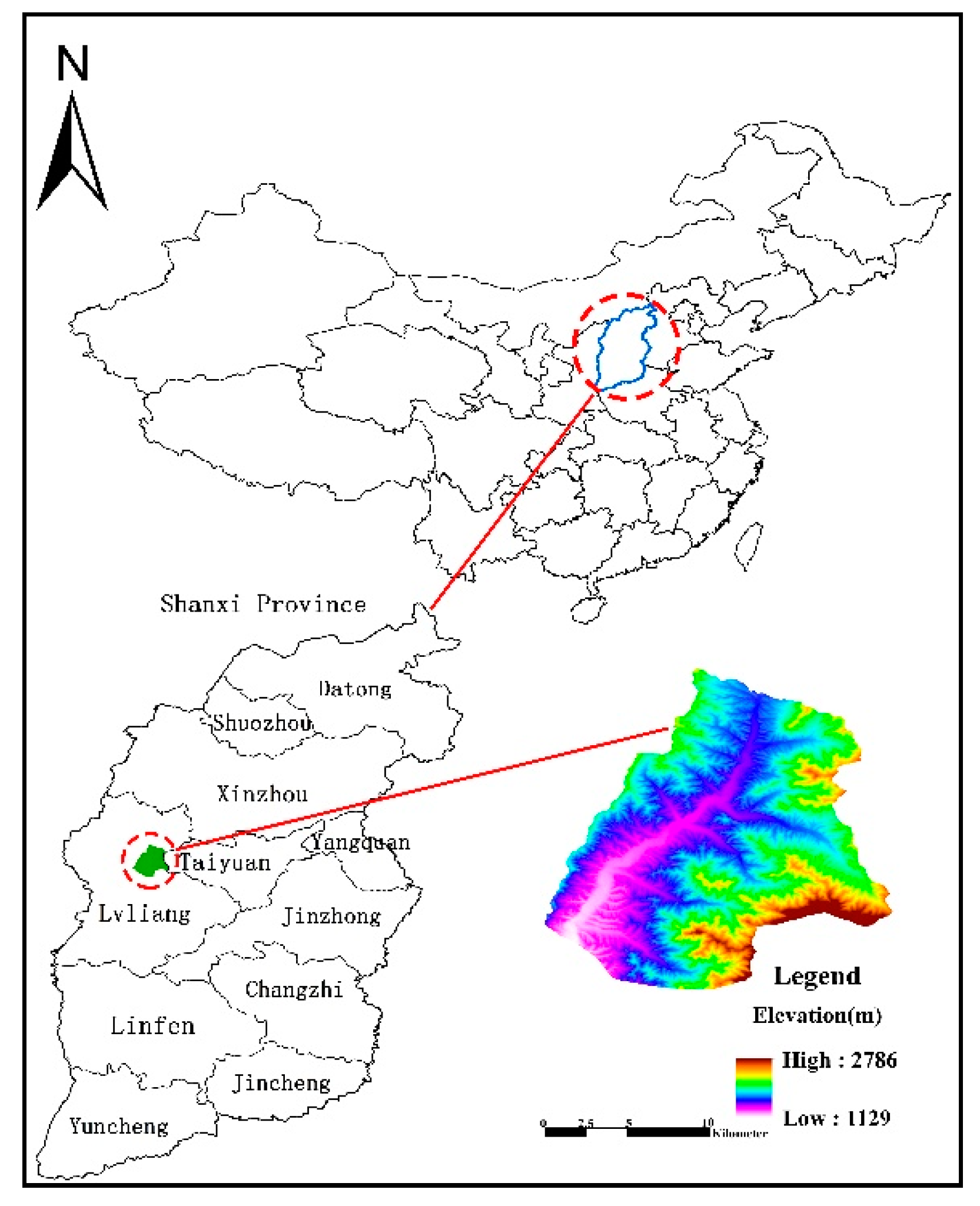
2. Study Area
2.1. Characteristics of Underlying Surface
2.1.1. Geographical Position
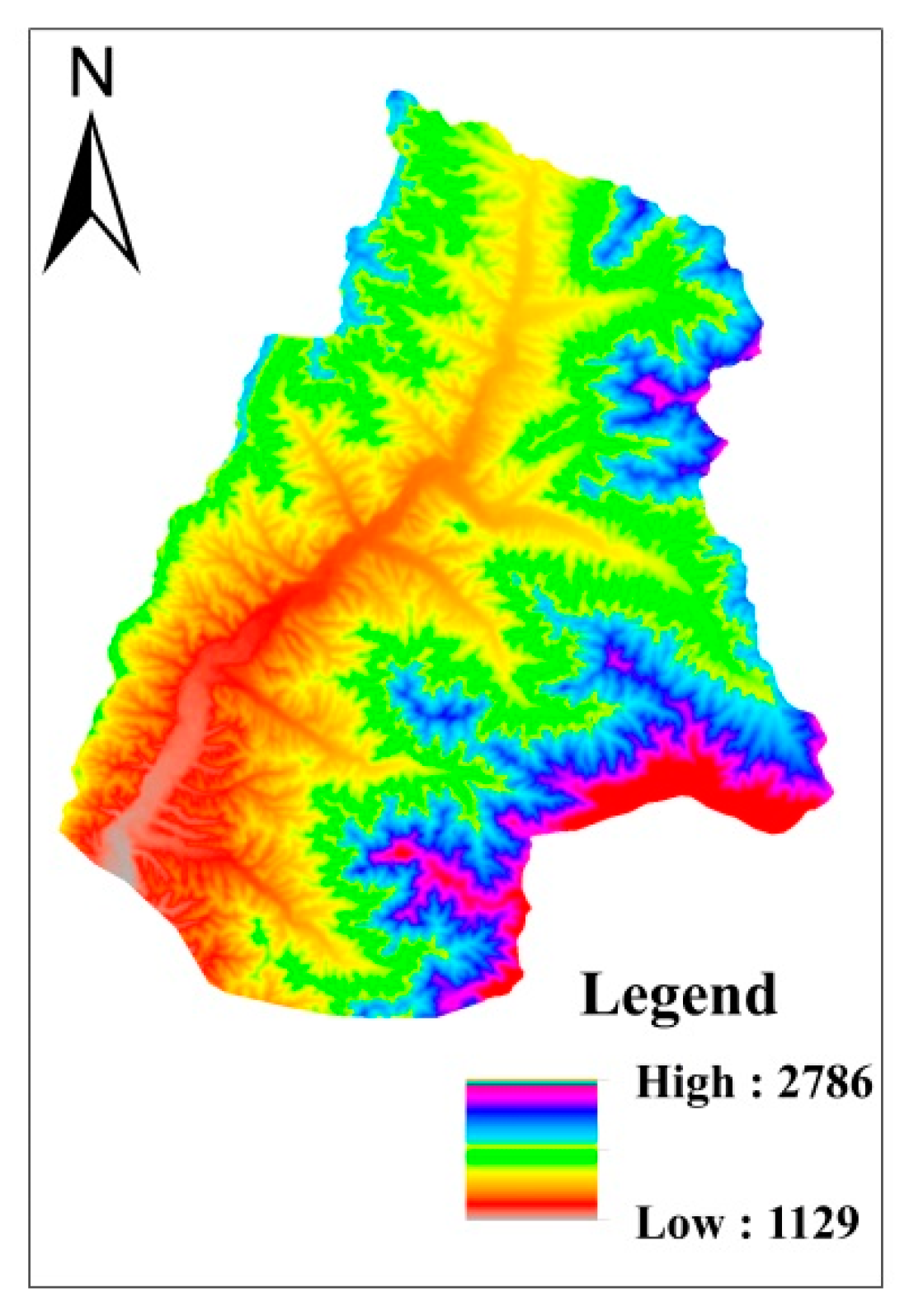
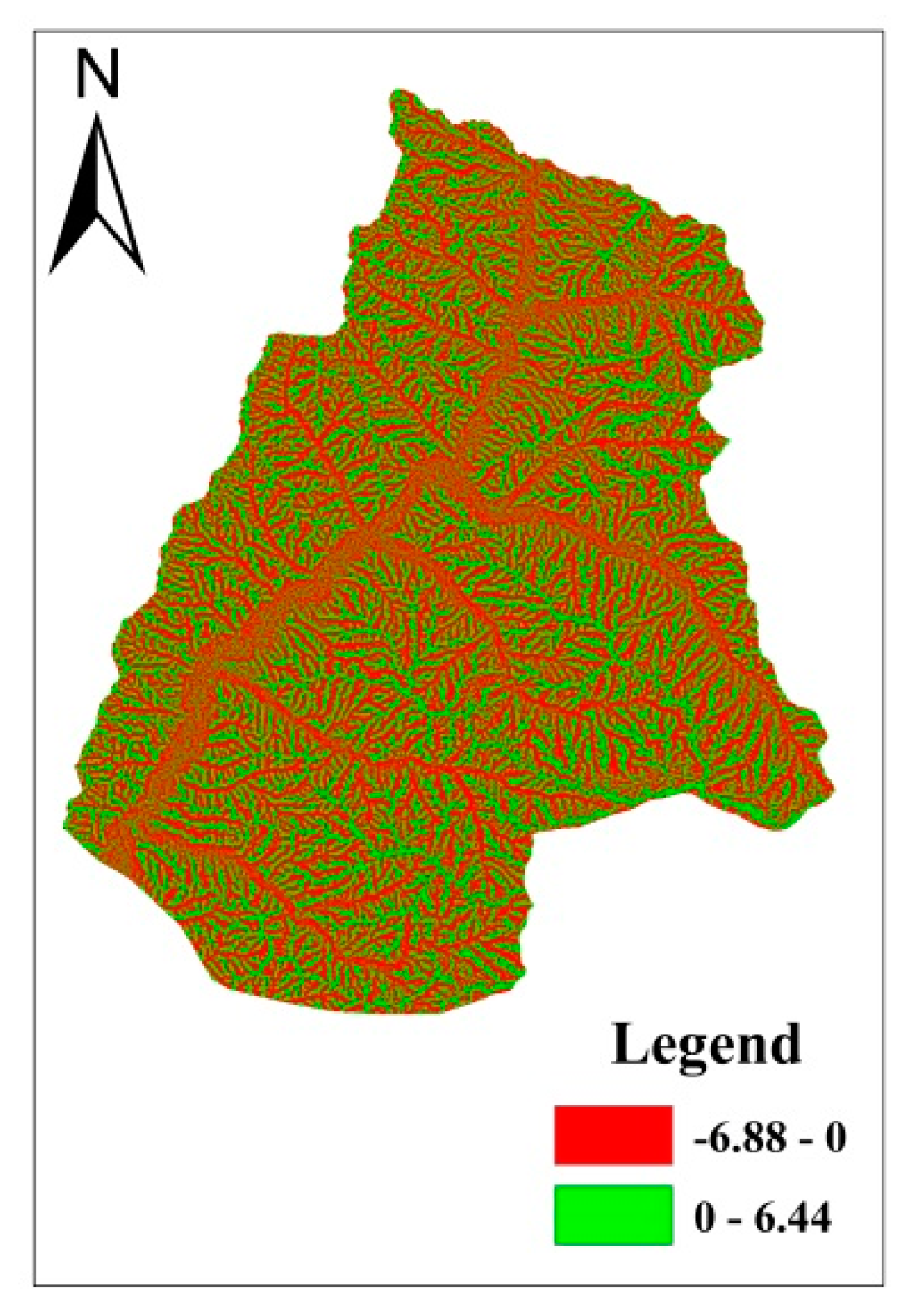
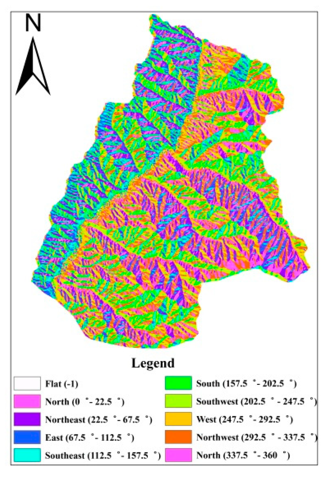
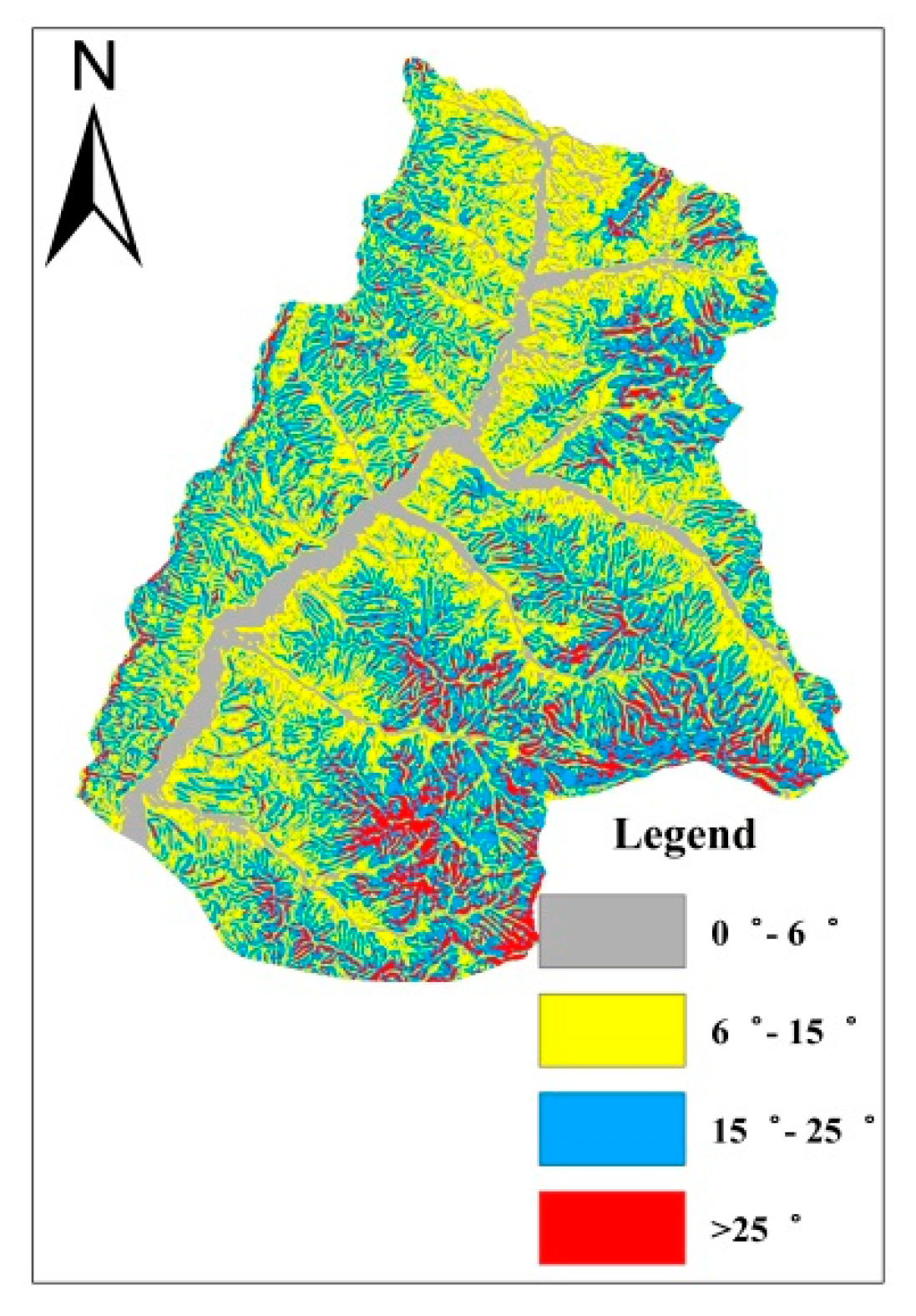
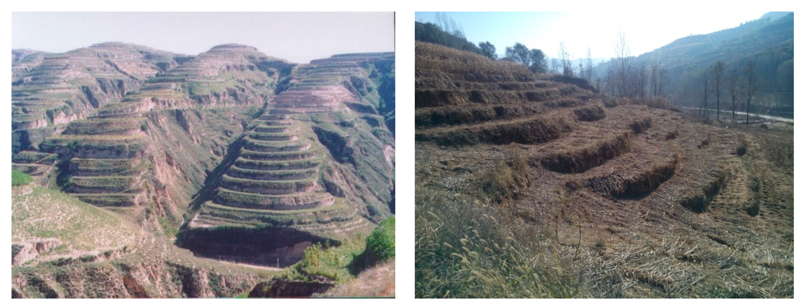
2.1.2. Topographical and Geomorphological Conditions
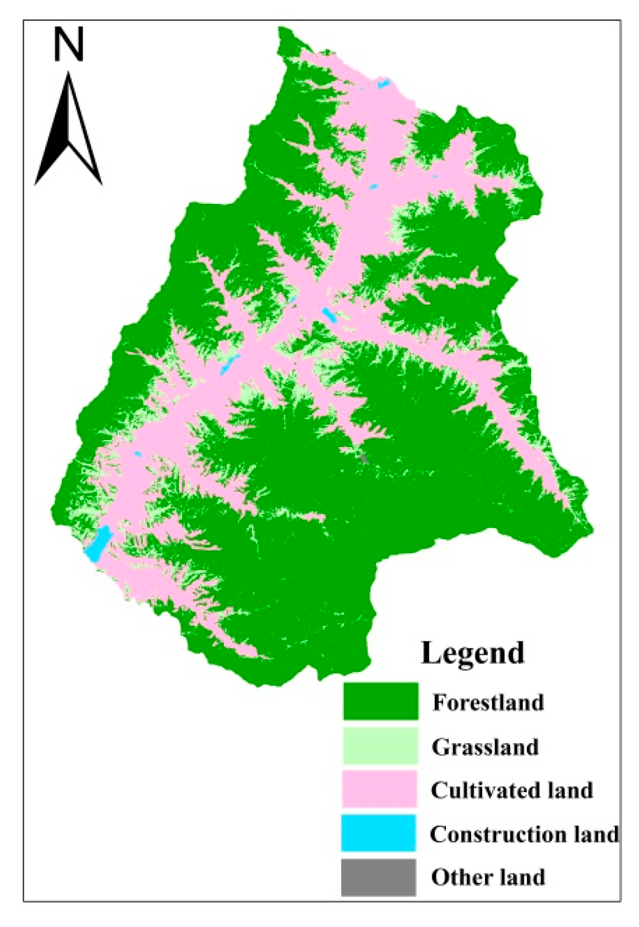
2.1.3. Soil and Land Use
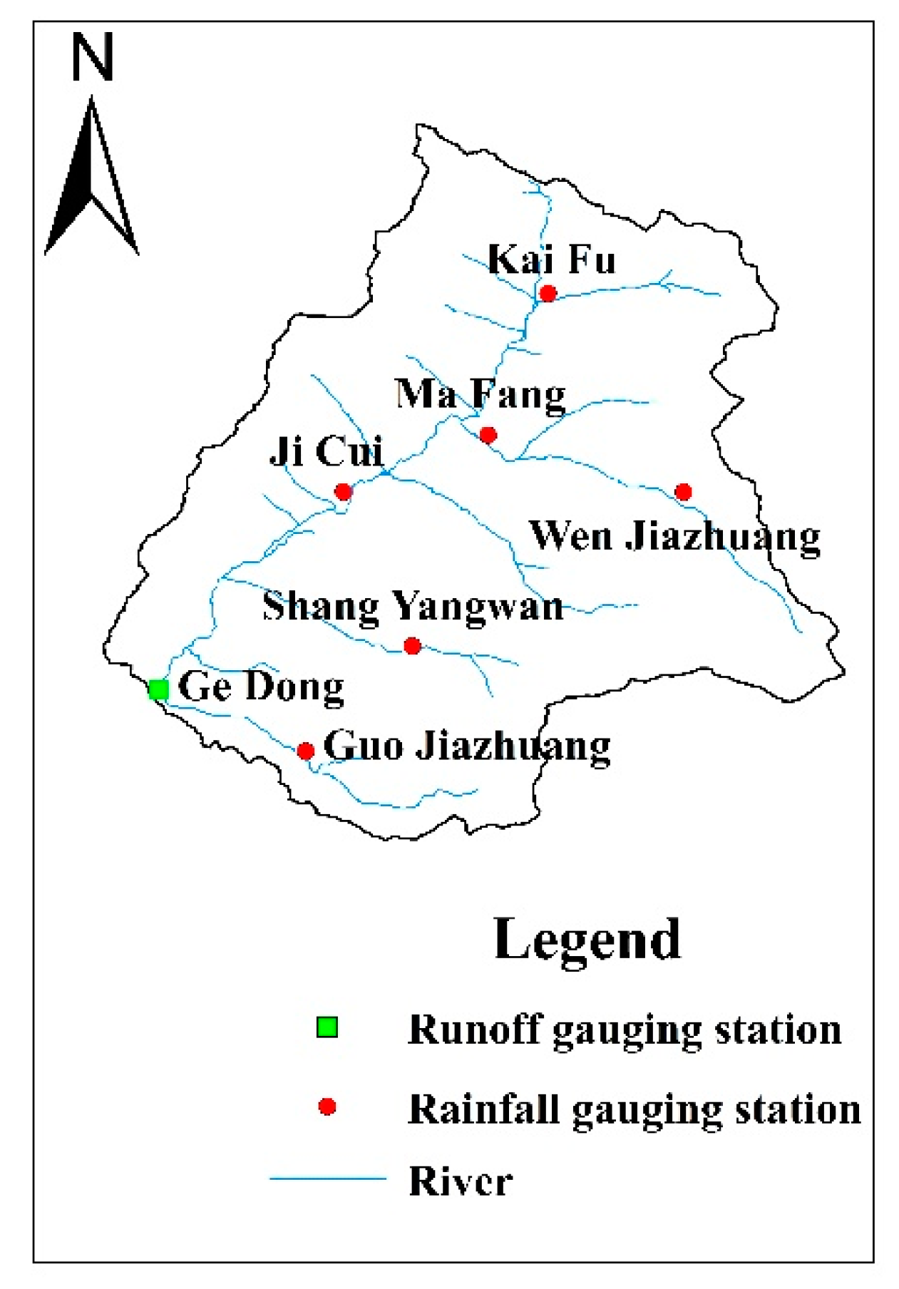
2.2. Meteorological and Hydrological Characteristics
2.2.1. Meteorological Characteristics
2.2.2. Hydrological Characteristics
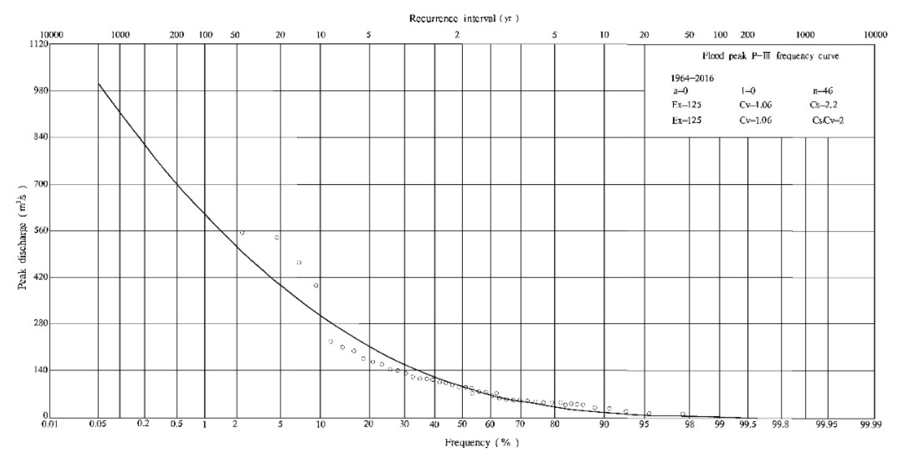
2.2.3. Flood Frequency Distribution Characteristics
3. Materials and Methods
3.1. Principle of ELM
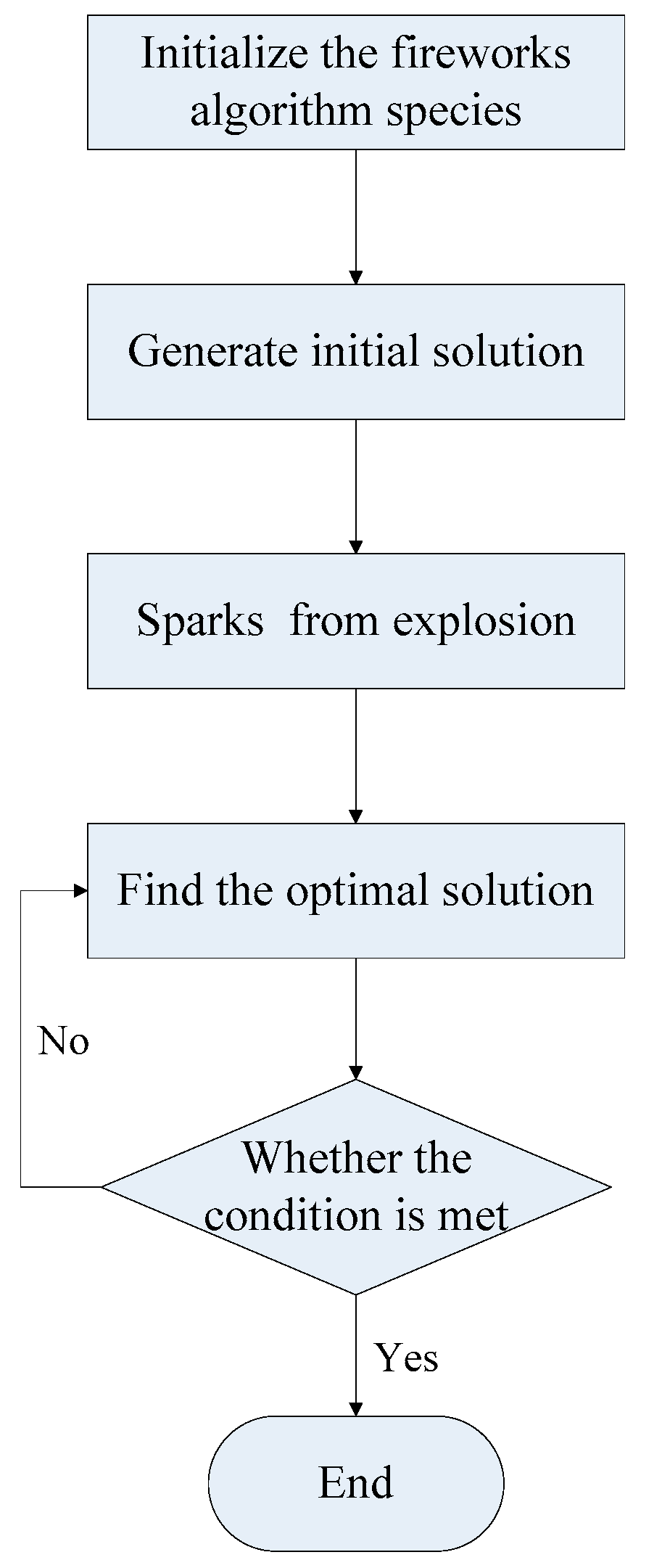
3.2. Principle of Fireworks Algorithm
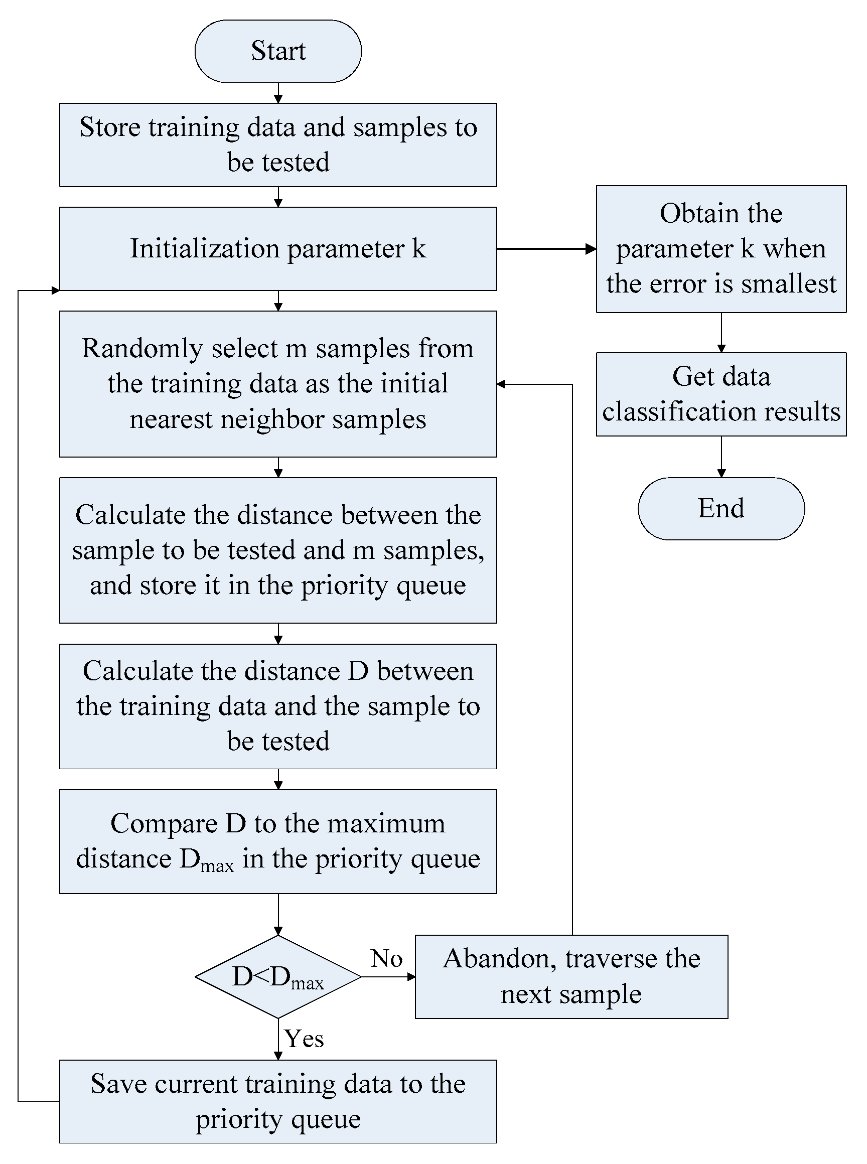
3.3. Principle of K Nearest Neighbor Method
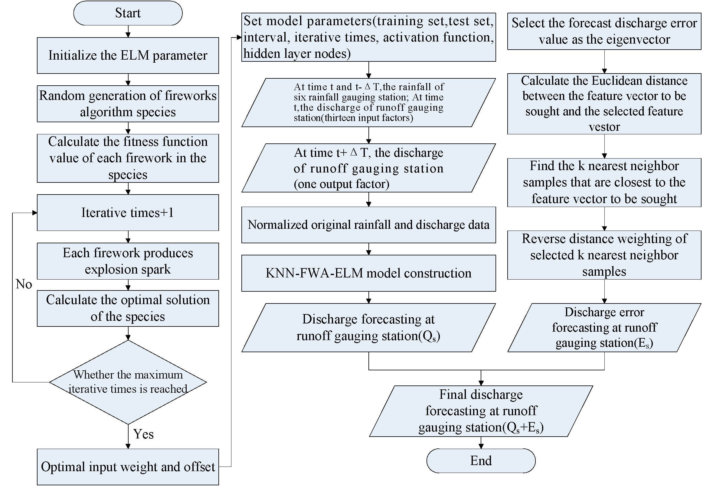
3.4. The Construction of the KNN-FWA-ELM Model
3.4.1. Model Parameters Setting
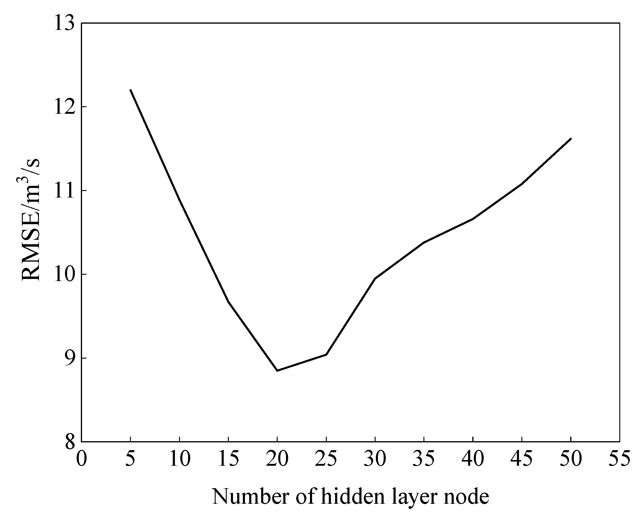
- (1)
- Set fewer hidden layer nodes;
- (2)
- Train and test the sample set;
- (3)
- Gradually increase the number of hidden layer nodes and use the same sample set for training and testing;
- (4)
- Compare the training and testing results of different hidden layer nodes, and obtain the number of hidden layer nodes when the error is the smallest.
3.4.2. Input and Output of the Model
- (1)
- Based on the analysis of the characteristics of the floods in HSP1, HSP2, and HSP3, obtain the average lag time of the floods in three periods, which is 1.07 h, 1.60 h, and 2.37 h, respectively, and ensure the maximum value of the ΔT is slightly larger than the average lag time of the floods in three periods, respectively.
- (2)
- Use the rainfall at each rainfall station at time t, at a certain early time, and the discharge at the outlet at time t as the input variables of the model, and ensure the maximum value of the period by which the rainfall shifted to a certain early time is the maximum value determined in the previous step.
- (3)
- Set the foregoing input variables as the input data and the discharge at the outlet at a certain late time corresponding to time t as the output data, make the iterative calculation by PMI method, and obtain the screened input variables, of which the difference between the corresponding time and time t is ΔT.
3.4.3. Data Normalization
3.4.4. Model Construction
3.4.5. Evaluation Indexes for Forecasting Performance
4. Results and Discussion
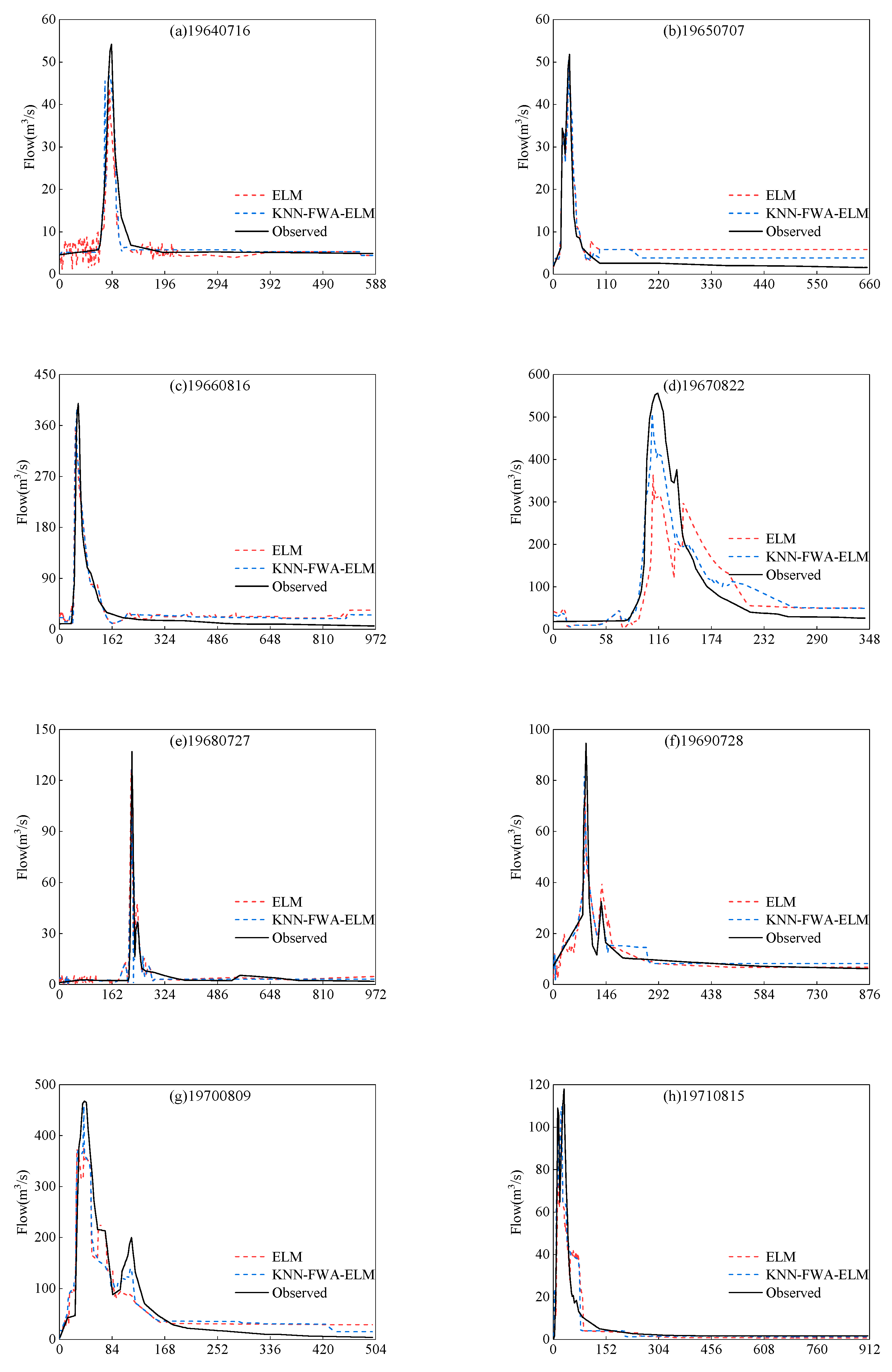
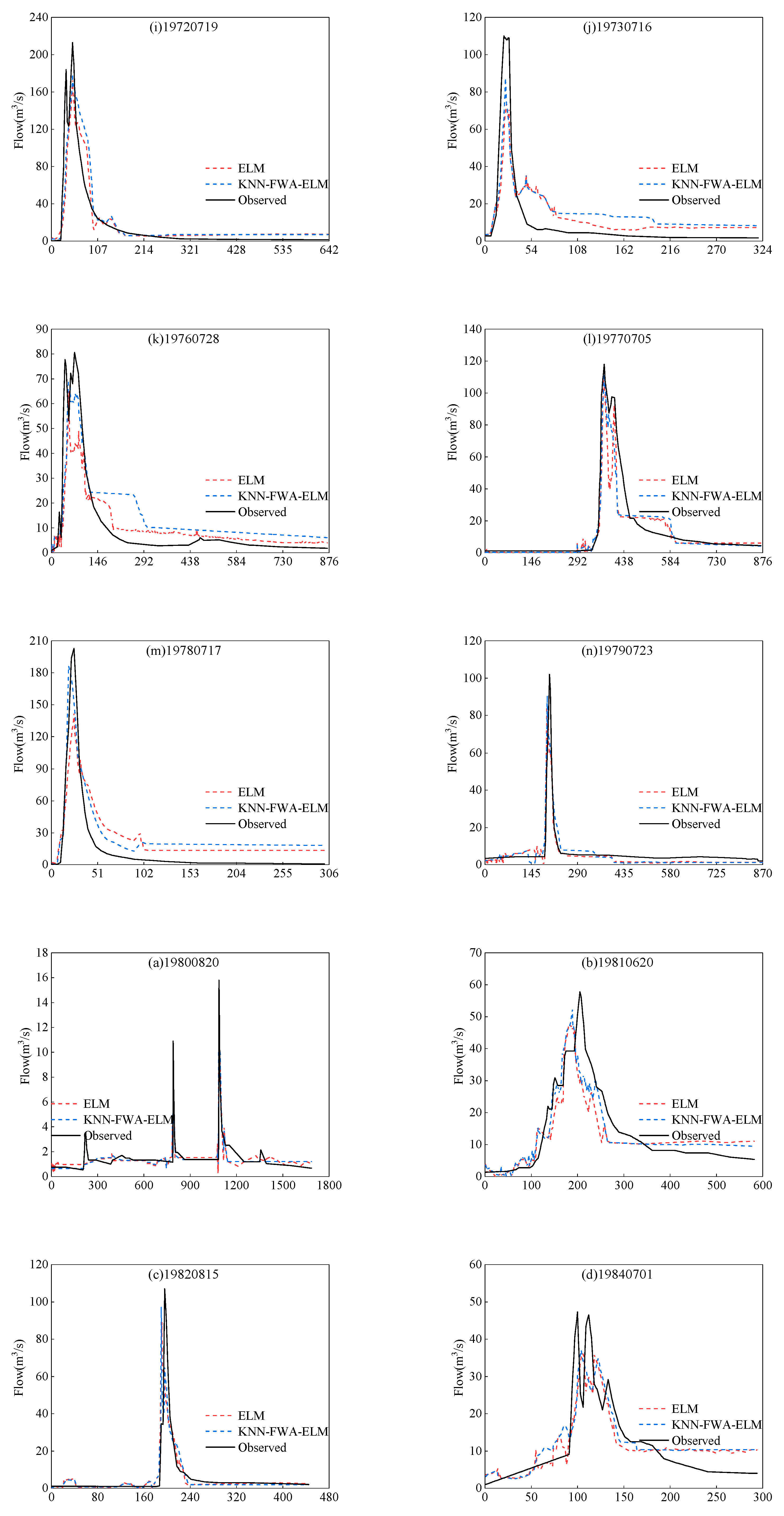
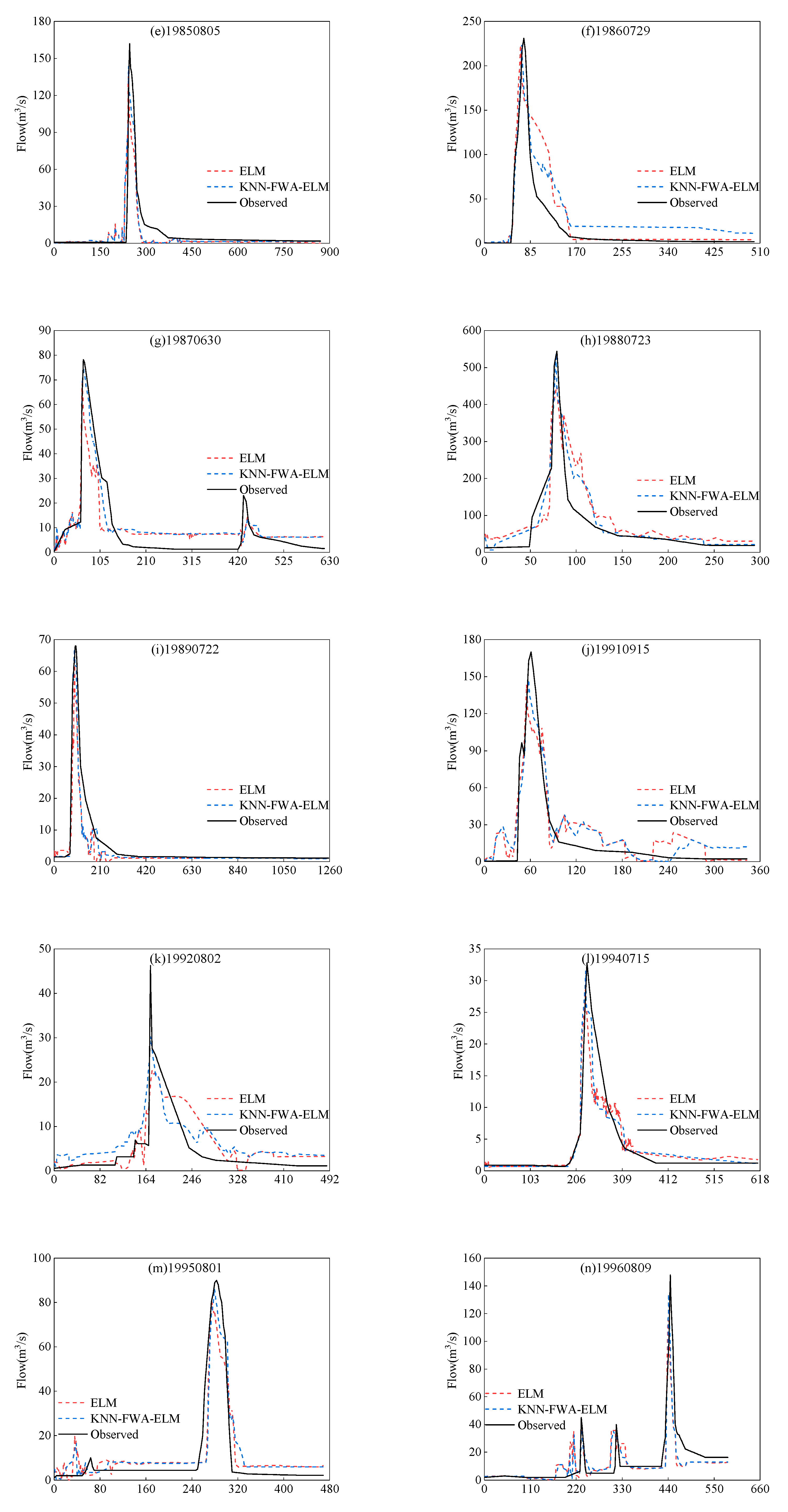
4.1. The Flood Forecasting of ELM Model
4.2. The Flood Forecasting of KNN-FWA-ELM Model
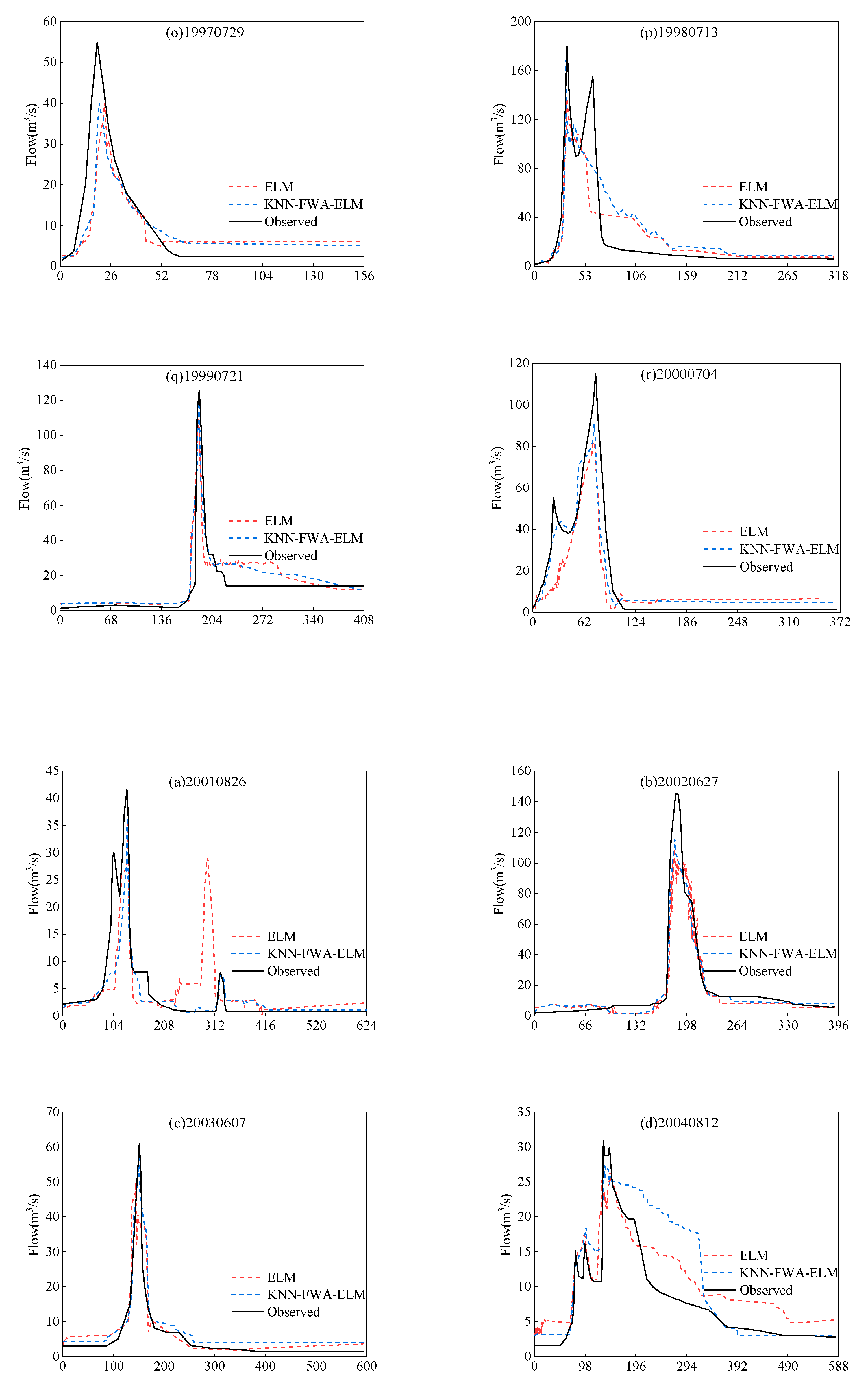
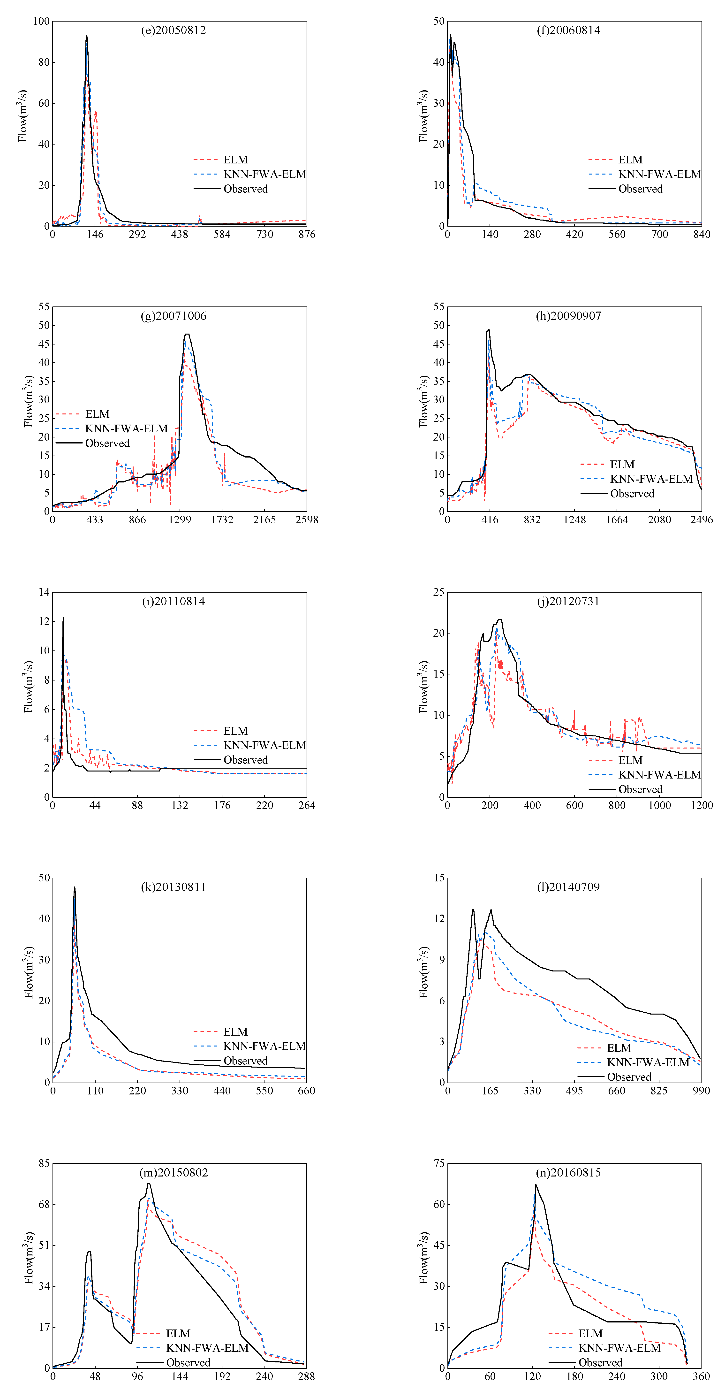
4.3. Comparison and Analysis of Simulation Results Between KNN-FWA-ELM Model and ELM Model
4.3.1. Comparison and Analysis of Simulation Results of All Floods
4.3.2. Comparison of Simulation Results of Floods in Different Periods
4.3.3. Comparison of Simulation Results of Floods Under Different Grades
5. Conclusions
Author Contributions
Funding
Acknowledgments
Conflicts of Interest
References
- Sun, Y.X.; Tang, D.S.; Sun, Y.F.; Cui, Q.F. Comparison of a fuzzy control and the data-driven model for flood forecasting. Nat. Hazards 2016, 82, 827–844. [Google Scholar] [CrossRef]
- Zhou, Y.L.; Guo, S.L.; Chang, F.J. Explore an evolutionary recurrent ANFIS for modeling multi-step-ahead flood forecasts. J. Hydrol. 2019, 570, 343–355. [Google Scholar] [CrossRef]
- Nguyen, P.K.T.; Chua, L.H.C.; Son, L.H. Flood forecasting in large rivers with data-driven models. Nat. Hazards 2014, 71, 767–784. [Google Scholar] [CrossRef]
- Badrzadeh, H.; Sarukkalige, R.; Jayawardena, A.W. Hourly runoff forecasting for flood risk management: Application of various computational intelligence models. J. Hydrol. 2015, 529, 1633–1643. [Google Scholar] [CrossRef]
- Seo, Y.M.; Kim, S.W.; Singh, V.J. Multistep-ahead flood forecasting using wavelet and data-driven methods. KSCE J. Civ. Eng. 2015, 19, 401–417. [Google Scholar] [CrossRef]
- Amirian, E.; Deiam, M.; Chen, Z.X. Performance forecasting for polymer flooding in heavy oil reservoirs. Fuel 2018, 216, 83–100. [Google Scholar] [CrossRef]
- Nguyen, P.K.T.; Chua, L.H.C. The data-driven approach as an operational real-time flood forecasting model. Hydrol. Process. 2012, 26, 2878–2893. [Google Scholar] [CrossRef]
- Matos, J.P.; Portela, M.M.; Schleiss, A.J. Towards safer data-driven forecasting of extreme streamflows. Water Resour. Manag. 2018, 32, 701–720. [Google Scholar] [CrossRef]
- Lima, A.R.; Cannon, A.J.; Hsieh, W.W. Nonlinear regression in environmental sciences using extreme learning machines: A comparative evaluation. Envrion. Model. Softw. 2015, 73, 175–188. [Google Scholar] [CrossRef]
- Hsieh, W.W. Machine Learning Methods in the Environmental Sciences; Cambridge University Press: Cambridge, England, 2009. [Google Scholar]
- Cherkassky, V.; Krasnopolsky, V.; Solomatine, D.P. Computational intelligence in earth sciences and environmental applications: Issues and challenges. Neural Netw. 2006, 19, 113–121. [Google Scholar] [CrossRef]
- Shamseldin, A.Y. Artificial neural network model for river flow forecasting in a developing country. J. Hydroinform. 2010, 12, 22–35. [Google Scholar] [CrossRef]
- Maier, H.R.; Jain, A.; Dandy, G.C. Methods used for the development of neural networks for the prediction of water resource variables in river systems: Current status and future directions. Environ. Model. Softw. 2010, 25, 891–909. [Google Scholar] [CrossRef]
- Chang, F.J.; Chen, P.A.; Lu, Y.R. Real-time multi-step-ahead water level forecasting by recurrent neural networks for urban flood control. J. Hydrol. 2014, 517, 836–846. [Google Scholar] [CrossRef]
- Wu, W.; Dandy, G.C.; Maier, H.R. Protocol for developing ANN models and its application to the assessment of the quality of the ANN model development process in drinking water quality modeling. Environ. Model. Softw. 2014, 54, 108–127. [Google Scholar] [CrossRef]
- Siqueira, H.; Boccato, L.; Attux, R. Echo state networks and extreme learning machines: A comparative study on seasonal streamflow series prediction. In Neural Information Processing, Proceedings of the International Conference on Neural Information Processing, Doha, Qatar, 12–15 November 2012; Springer: Berlin/Heidelberg, Germany, 2012; pp. 491–500. [Google Scholar]
- Hadi, S.J.; Tombul, M. Forecasting daily streamflow for basins with different physical characteristics through data-driven methods. Water Resour. Manag. 2018, 32, 3405–3422. [Google Scholar] [CrossRef]
- He, Z.; Wen, X.; Liu, H. A comparative study of artificial neural network, adaptive neuro fuzzy inference system and support vector machine for forecastinging river flow in the semiarid mountain region. J. Hydrol. 2014, 509, 379–386. [Google Scholar] [CrossRef]
- Taormina, R.; Chau, K.W. Data-driven input variable selection for rainfall–runoff modeling using binary-coded particle swarm optimization and Extreme Learning Machines. J. Hydrol. 2015, 529, 1617–1632. [Google Scholar] [CrossRef]
- Lima, A.R.; Cannon, A.J.; Hsieh, W.W. Forecasting daily streamflow using online sequential extreme learning machines. J. Hydrol. 2016, 537, 431–443. [Google Scholar] [CrossRef]
- Wang, J.J.; Shi, P.; Jiang, P. Application of BP Neural Network Algorithm in Traditional Hydrological Model for Flood Forecasting. Water 2017, 9, 48. [Google Scholar] [CrossRef]
- Kong, J.; Li, S.J.; Zhu, Y.L. Flood forecasting for small and medium-sized rivers by ensemble extreme learning machine. J. Hydrol. 2018, 38, 67–72. (In Chinese) [Google Scholar]
- Liu, J. The application of parallel extreme learning machine in flood forecasting. J. Northwest. Univ. (Nat. Sci. Ed.) 2015, 45, 545–550. (In Chinese) [Google Scholar]
- Kan, G.Y.; Hong, Y.; Liang, K. Research on the flood forecasting based on coupled machine learning model. China Rural Water Hydropower 2018, 10, 165–169. (In Chinese) [Google Scholar]
- Huang, G.B.; Zhu, Q.Y.; Siew, C.K. Extreme learning machine: Theory and applications. Neurocomputing 2006, 70, 489–501. [Google Scholar] [CrossRef]
- Abdullah, S.S.; Malek, M.A.; Abdullah, N.S.; Kisi, O.; Yap, K.S. Extreme learning machines: A new approach for prediction of reference evapotranspiration. J. Hydrol. 2015, 527, 184–195. [Google Scholar] [CrossRef]
- Wan, C.; Song, Y.H.; Xu, Z.; Yang, G.Y.; Nielsen, A.H. Probabilistic wind power forecasting with hybid artificial netural networks. Electr. Power Compon. Syst. 2016, 44, 1656–1668. [Google Scholar] [CrossRef]
- Bai, Y.; Chen, Z.Q.; Xie, J.J. Daily reservoir inflow forecasting using multiscale deep feature learning with hybrid models. J. Hydrol. 2016, 532, 193–206. [Google Scholar] [CrossRef]
- Deo, R.C.; Tiwari, M.K.; Adamowski, J.F.; Quilty, J.M. Forecasting effective drought index using a wavelet extreme learning machine (W-ELM) model. Stoch. Envrion. Res. Risk Assess. 2017, 31, 1211–1240. [Google Scholar] [CrossRef]
- Ali, M.; Deo, R.C.; Downs, N.J.; Maraseni, T. Multi-stage committee based extreme learning machine model incorporating the influence of climate parameters and seasonality on drought forecasting. Comput. Electron. Agric. 2018, 152, 149–165. [Google Scholar] [CrossRef]
- Wang, W.Z.; Jiao, J.Y. Statistic analysis on process of gully runoff and sediment yield under different rain pattern in Loess Plateau Region. Bull. Soil Water Conserv. 1996, 16, 12–18. (In Chinese) [Google Scholar]
- Zhang, Y.C.; Liu, C.M.; Yang, S.T.; Liu, X.Y.; Cai, M.Y.; Dong, G.T.; Luo, Y. Comparison of LCM hydrological models with lumped, semi-distributed and distributed building structures in typical watershed of Yellow River Basin. Acta Geogr. Sin. 2014, 69, 90–99. (In Chinese) [Google Scholar]
- Li, J. Study on Flood Runoff Variation Characteristics in Dalin River Basin. Master’s Thesis, Xi’an University of Techonology, Xi’an, China, June 2017. (In Chinese). [Google Scholar]
- Yang, H. Analysis on the Causes and Characteristics of River Runoff Change in Beiyuhe Basin. Master’s Thesis, Lanzhou University, Lanzhou, China, May 2018. (In Chinese). [Google Scholar]
- Feng, X.W. Prediction of Secondary Flood in Semi-Arid Area Based on Multiple Combination Models. Master’s Thesis, Xi’an University of Techonology, Xi’an, China, June 2018. (In Chinese). [Google Scholar]
- Ren, J.H.; Zheng, X.Q.; Zhao, X.H.; Chen, J.F.; Li, A.M.; Chen, Y.P. Characteristics of flood evolution and their contribution factors in Gedong basin of loess hilly region in Western Shanxi Province. Water Res. Power. 2017, 35, 47–50. (In Chinese) [Google Scholar]
- Huang, G.B.; Zhou, H.; Ding, X. Extreme learning machine for regression and multiclass classification. IEEE Trans. Syst. Man Cybern. Part B Cybern. 2012, 42, 513–529. [Google Scholar] [CrossRef]
- Zhu, Q.Y.; Qin, A.K.; Suganthan, P.N. Evolutionary extreme learning machine. Pattern Recognit. 2005, 38, 1759–1763. [Google Scholar] [CrossRef]
- Huang, G.B.; Ding, X.; Zhou, H. Optimization method based extreme learning machine for classification. Neurocomputing 2010, 74, 155–163. [Google Scholar] [CrossRef]
- Tan, Y.; Zhu, Y. Fireworks Algorithm for Optimization. In Proceedings of the International Conference on Advances in Swarm Intelligence, Berlin, Germany, 12–15 June 2010; pp. 355–364. [Google Scholar]
- Cheng, S.; Qin, Q.; Chen, J. Analytics on Fireworks Algorithm Solving Problems with Shifts in the Decision Space and Objective Space. Int. J. Swarm Intell. Res. 2015, 6, 52–86. [Google Scholar] [CrossRef]
- Altman, N.S. An Introduction to Kernel and Nearest-Neighbor Nonparametric Regression. Am. Stat. 1992, 46, 175–185. [Google Scholar] [Green Version]
- Huang, Y.W.; Lai, D.H. Hidden Node Optimization for Extreme Learning Machine. AASRI Procedia 2012, 3, 375–380. [Google Scholar] [CrossRef]
- Sharma, A. Seasonal to interannual rainfall probabilistic forecastings for improved water supply management: Part 1—A strategy for system predictor identification. J. Hydrol. 2000, 239, 232–239. [Google Scholar] [CrossRef]
- Sharma, A.; Luk, K.C.; Cordery, I. Seasonal to interannual rainfall probabilistic forecastings for improved water supply management: Part 2—Predictor identification of quarterly rainfall using ocean-atmosphere information. J. Hydrol. 2000, 239, 240–248. [Google Scholar] [CrossRef]
- Sharma, A. Seasonal to interannual rainfall probabilistic forecastings for improved water supply management: Part 3—A nonparametric probabilistic forecasting model. J. Hydrol. 2000, 239, 249–258. [Google Scholar] [CrossRef]
- Dawson, C.W.; Abrahart, R.J.; See, L.M. HydroTest: A web-based toolbox of evaluation metrics for the standardized assessment of hydrological forecasts. Envrion. Model. Softw. 2007, 22, 1034–1052. [Google Scholar] [CrossRef]
- Jain, A.; Srinivasulu, S. Development of effective and efficient rainfall-runoff models using integration of deterministic, real-coded genetic algorithms and artificial neural network techniques. Water Resour. Res. 2004. [Google Scholar] [CrossRef]
- Dawson, C.W.; Wilby, R.L. Hydrological modelling using artificial neural networks. Prog. Phys. Geogr. 2001, 25, 80–108. [Google Scholar] [CrossRef]
- Zhang, D.H.; Zhang, J.C.; Liu, F.G. Some comments on nonlinear effect in catchment hydrology. Adv. Water Sci. 2007, 5, 776–784. (In Chinese) [Google Scholar]


| Land Use Type | 1987 | 1990 | 1996 | |||
| Area (km2) | Percentage (%) | Area (km2) | Percentage (%) | Area (km2) | Percentage (%) | |
| Forestland | 313.56 | 43.31 | 333.33 | 46.04 | 334.13 | 46.15 |
| Grassland | 124.96 | 17.26 | 130.46 | 18.02 | 142.34 | 19.66 |
| Cultivated land | 255.43 | 35.28 | 242.32 | 33.48 | 220.60 | 30.47 |
| Construction land | 3.48 | 0.48 | 5.14 | 0.71 | 5.57 | 0.77 |
| Other land | 26.57 | 3.67 | 12.74 | 1.75 | 21.36 | 2.95 |
| Land Use type | 2003 | 2007 | 2012 | |||
| Area (km2) | Percentage (%) | Area (km2) | Percentage (%) | Area (km2) | Percentage (%) | |
| Forestland | 393.28 | 54.32 | 410.80 | 56.74 | 441.93 | 61.04 |
| Grassland | 158.41 | 21.88 | 159.42 | 22.02 | 174.05 | 24.04 |
| Cultivated land | 149.43 | 20.64 | 128.22 | 17.71 | 84.27 | 11.64 |
| Construction land | 13.18 | 1.82 | 18.17 | 2.51 | 23.53 | 3.25 |
| Other land | 9.70 | 1.34 | 7.39 | 1.02 | 0.22 | 0.03 |
| Flood Grade | Flood Recurrence Interval (Year) | Flood Frequency (%) | Flood Type |
|---|---|---|---|
| 1 | <5 | >20 | small |
| 2 | 5–10 | 10–20 | moderate |
| 3 | 10–50 | 2–10 | great |
| 4 | 50–100 | 1–2 | extraordinary |
| 5 | >100 | <1 | abnormal |
| Periods | Data Set | Flood Events | ΔQ/% | Δh/h | NS | R2 | RMSE/m3/s | MSRE | MARE | Qualified or Not |
|---|---|---|---|---|---|---|---|---|---|---|
| HSP1 | Training | 19640716 | −19.21 | −0.33 | 0.83 | 0.91 | 2.86 | 0.05 | 0.17 | Qualified |
| Training | 19670822 | −34.43 | −0.42 | 0.60 | 0.63 | 85.43 | 0.48 | 0.65 | Not qualified | |
| Training | 19680727 | −7.15 | −0.17 | 0.78 | 0.78 | 5.19 | 0.67 | 0.56 | Qualified | |
| Training | 19690728 | −17.24 | −0.25 | 0.79 | 0.79 | 4.39 | 0.04 | 0.16 | Qualified | |
| Training | 19700809 | −19.18 | −0.08 | 0.86 | 0.89 | 36.59 | 3.15 | 0.92 | Qualified | |
| Training | 19710815 | −10.27 | −0.50 | 0.81 | 0.82 | 7.30 | 1.16 | 0.57 | Qualified | |
| Training | 19720719 | −18.69 | 0 | 0.82 | 0.83 | 15.19 | 6.09 | 1.04 | Qualified | |
| Training | 19730716 | −32.93 | 0.25 | 0.64 | 0.75 | 11.92 | 4.64 | 1.92 | Not qualified | |
| Training | 19760728 | −19.55 | −1.50 | 0.72 | 0.83 | 9.08 | 1.01 | 0.46 | Qualified | |
| Training | 19780717 | −29.89 | 0 | 0.69 | 0.85 | 19.51 | 17.63 | 2.66 | Not qualified | |
| Testing | 19650707 | −5.93 | −0.17 | 0.70 | 0.94 | 3.67 | 2.19 | 1.09 | Qualified | |
| Testing | 19660816 | −10.89 | −0.75 | 0.83 | 0.88 | 19.88 | 2.02 | 0.86 | Qualified | |
| Testing | 19770705 | −7.58 | −0.25 | 0.81 | 0.86 | 10.26 | 0.37 | 0.53 | Qualified | |
| Testing | 19790723 | −16.01 | −0.67 | 0.83 | 0.85 | 4.37 | 0.30 | 0.39 | Qualified | |
| HSP2 | Training | 19800820 | −34.75 | −0.17 | 0.66 | 0.66 | 0.62 | 0.15 | 0.29 | Not qualified |
| Training | 19840701 | −23.62 | 0.42 | 0.67 | 0.69 | 5.69 | 0.70 | 0.61 | Not qualified | |
| Training | 19850805 | −14.02 | −0.42 | 0.76 | 0.79 | 10.40 | 36.65 | 1.43 | Qualified | |
| Training | 19860729 | −3.33 | −0.50 | 0.68 | 0.80 | 22.72 | 6.55 | 4.27 | Not qualified | |
| Training | 19880723 | −17.22 | 0 | 0.66 | 0.74 | 53.29 | 1.48 | 0.89 | Not qualified | |
| Training | 19910915 | −15.80 | −0.50 | 0.80 | 0.84 | 15.62 | 131.22 | 4.93 | Qualified | |
| Training | 19920802 | −51.04 | 0.25 | 0.65 | 0.70 | 3.82 | 2.92 | 1.49 | Not qualified | |
| Training | 19940715 | −12.87 | −0.33 | 0.82 | 0.84 | 2.54 | 0.26 | 0.42 | Qualified | |
| Training | 19950801 | −10.67 | −0.67 | 0.84 | 0.87 | 8.02 | 2.43 | 1.16 | Qualified | |
| Training | 19960809 | −19.96 | −0.42 | 0.65 | 0.67 | 11.11 | 2.13 | 0.74 | Not qualified | |
| Training | 19970729 | −27.15 | 0.33 | 0.64 | 0.72 | 6.92 | 1.38 | 1.06 | Not qualified | |
| Training | 19990721 | −12.76 | −0.17 | 0.71 | 0.74 | 9.20 | 0.61 | 0.61 | Qualified | |
| Training | 20000704 | −28.59 | −0.25 | 0.76 | 0.82 | 12.05 | 7.41 | 2.39 | Not qualified | |
| Testing | 19810620 | −17.70 | −1.75 | 0.72 | 0.74 | 6.60 | 0.28 | 0.44 | Qualified | |
| Testing | 19820815 | −16.70 | −0.42 | 0.70 | 0.70 | 7.05 | 1.89 | 0.69 | Qualified | |
| Testing | 19870630 | −10.68 | −0.25 | 0.72 | 0.81 | 7.92 | 8.11 | 2.14 | Qualified | |
| Testing | 19890722 | −8.84 | −0.25 | 0.81 | 0.91 | 4.41 | 0.18 | 0.30 | Qualified | |
| Testing | 19980713 | −23.91 | 0 | 0.69 | 0.71 | 20.36 | 0.81 | 0.69 | Not qualified | |
| HSP3 | Training | 20010826 | −14.62 | 0.17 | 0.32 | 0.36 | 6.02 | 2.84 | 1.61 | Not qualified |
| Training | 20030607 | −18.50 | −0.58 | 0.79 | 0.81 | 3.81 | 1.68 | 0.67 | Qualified | |
| Training | 20040812 | −18.34 | −0.25 | 0.72 | 0.87 | 3.60 | 1.79 | 0.71 | Qualified | |
| Training | 20050812 | −14.09 | −0.25 | 0.80 | 0.80 | 6.00 | 2.28 | 1.07 | Qualified | |
| Training | 20071006 | −9.67 | −0.50 | 0.79 | 0.86 | 4.74 | 1.14 | 0.32 | Qualified | |
| Training | 20090907 | −14.99 | −0.42 | 0.73 | 0.81 | 5.22 | 1.04 | 0.15 | Qualified | |
| Training | 20110814 | −22.72 | 0 | 0.05 | 0.51 | 0.86 | 0.08 | 0.22 | Not qualified | |
| Training | 20130811 | −11.30 | 0 | 0.74 | 0.85 | 6.57 | 1.23 | 0.66 | Qualified | |
| Training | 20140709 | −17.32 | 2.42 | 0.36 | 0.71 | 2.66 | 0.13 | 0.34 | Not qualified | |
| Training | 20160815 | −11.87 | −0.07 | 0.78 | 0.79 | 9.23 | 1.21 | 0.69 | Qualified | |
| Testing | 20020627 | −24.65 | −0.17 | 0.87 | 0.90 | 100.38 | 0.49 | 0.52 | Not qualified | |
| Testing | 20060814 | −6.28 | −0.25 | 0.79 | 0.84 | 4.25 | 2.23 | 1.11 | Qualified | |
| Testing | 20120731 | −6.75 | −0.75 | 0.72 | 0.75 | 2.60 | 2.08 | 0.18 | Qualified | |
| Testing | 20150802 | −9.13 | 0 | 0.72 | 0.73 | 11.80 | 1.18 | 0.72 | Qualified |
| Periods | Data Set | Flood Events | ΔQ/% | Δh/h | NS | R2 | RMSE/m3/s | MSRE | MARE | Qualified or Not |
|---|---|---|---|---|---|---|---|---|---|---|
| HSP1 | Training | 19640716 | −13.67 | −0.33 | 0.91 | 0.91 | 2.04 | 0.02 | 0.09 | Qualified |
| Training | 19660816 | −2.27 | −0.42 | 0.86 | 0.90 | 18.06 | 1.43 | 0.61 | Qualified | |
| Training | 19670822 | −8.58 | −0.50 | 0.89 | 0.95 | 43.18 | 0.31 | 0.49 | Qualified | |
| Training | 19680727 | −6.25 | 0 | 0.84 | 0.84 | 4.35 | 0.40 | 0.39 | Qualified | |
| Training | 19690728 | −13.33 | −0.42 | 0.84 | 0.85 | 3.79 | 0.04 | 0.12 | Qualified | |
| Training | 19710815 | −8.26 | 0 | 0.85 | 0.85 | 6.54 | 0.68 | 0.30 | Qualified | |
| Training | 19720719 | −15.87 | 0 | 0.86 | 0.86 | 13.59 | 4.36 | 0.73 | Qualified | |
| Training | 19730716 | −20.55 | 0.17 | 0.69 | 0.81 | 10.95 | 4.59 | 1.90 | Not qualified | |
| Training | 19760728 | −14.96 | −1.58 | 0.85 | 0.89 | 6.60 | 0.81 | 0.35 | Qualified | |
| Training | 19790723 | −11.15 | −0.58 | 0.85 | 0.88 | 4.05 | 0.25 | 0.28 | Qualified | |
| Testing | 19650707 | −2.70 | −0.17 | 0.87 | 0.94 | 2.40 | 0.74 | 0.74 | Qualified | |
| Testing | 19700809 | −2.09 | −0.08 | 0.88 | 0.91 | 32.72 | 2.01 | 0.75 | Qualified | |
| Testing | 19770705 | −3.42 | 0 | 0.86 | 0.89 | 8.65 | 0.31 | 0.40 | Qualified | |
| Testing | 19780717 | −8.24 | −0.50 | 0.82 | 0.93 | 14.88 | 8.78 | 1.35 | Qualified | |
| HSP2 | Training | 19800820 | −9.43 | −0.17 | 0.70 | 0.71 | 0.58 | 0.13 | 0.26 | Qualified |
| Training | 19820815 | −9.07 | −0.50 | 0.74 | 0.75 | 6.54 | 1.88 | 0.65 | Qualified | |
| Training | 19840701 | −21.65 | 0.33 | 0.69 | 0.70 | 5.55 | 0.65 | 0.60 | Not qualified | |
| Training | 19850805 | −11.33 | −0.33 | 0.83 | 0.84 | 8.83 | 33.29 | 1.33 | Qualified | |
| Training | 19860729 | −2.91 | −0.33 | 0.79 | 0.90 | 18.20 | 5.70 | 1.05 | Qualified | |
| Training | 19880723 | −1.03 | −0.08 | 0.84 | 0.87 | 36.44 | 0.68 | 0.49 | Qualified | |
| Training | 19910915 | −13.32 | −0.25 | 0.85 | 0.90 | 13.23 | 118.65 | 4.41 | Qualified | |
| Training | 19920802 | −34.51 | 0 | 0.67 | 0.79 | 3.76 | 1.48 | 0.99 | Not qualified | |
| Training | 19940715 | −3.90 | −0.25 | 0.87 | 0.87 | 2.22 | 0.24 | 0.36 | Qualified | |
| Training | 19950801 | −4.13 | −0.33 | 0.87 | 0.88 | 7.08 | 2.00 | 1.06 | Qualified | |
| Training | 19960809 | −9.40 | −0.33 | 0.70 | 0.70 | 10.36 | 1.85 | 0.68 | Qualified | |
| Training | 19970729 | −27.05 | 0.08 | 0.68 | 0.80 | 6.50 | 1.36 | 1.03 | Not qualified | |
| Training | 19990721 | −1.95 | 0 | 0.76 | 0.79 | 8.32 | 0.58 | 0.59 | Qualified | |
| Testing | 19810620 | −9.36 | −1.33 | 0.81 | 0.82 | 5.36 | 0.24 | 0.39 | Qualified | |
| Testing | 19870630 | −1.01 | 0 | 0.82 | 0.85 | 6.30 | 8.03 | 2.12 | Qualified | |
| Testing | 19890722 | −1.50 | −0.33 | 0.88 | 0.91 | 3.52 | 0.09 | 0.23 | Qualified | |
| Testing | 19980713 | −6.13 | −0.08 | 0.81 | 0.83 | 15.93 | 0.69 | 0.59 | Qualified | |
| Testing | 20000704 | −21.09 | −0.17 | 0.83 | 0.85 | 10.18 | 7.38 | 2.35 | Not qualified | |
| HSP3 | Training | 20020627 | −20.07 | −0.08 | 0.71 | 0.75 | 73.07 | 0.47 | 0.51 | Not qualified |
| Training | 20030607 | −4.21 | −0.08 | 0.85 | 0.85 | 3.38 | 1.52 | 0.51 | Qualified | |
| Training | 20040812 | −8.15 | 0 | 0.86 | 0.88 | 2.57 | 1.67 | 0.68 | Qualified | |
| Training | 20050812 | −3.88 | −0.17 | 0.84 | 0.87 | 5.27 | 1.98 | 0.90 | Qualified | |
| Training | 20060814 | −2.33 | −0.25 | 0.85 | 0.85 | 3.69 | 1.95 | 0.91 | Qualified | |
| Training | 20071006 | −3.75 | −0.25 | 0.86 | 0.88 | 4.04 | 1.13 | 0.26 | Qualified | |
| Training | 20090907 | −5.64 | −0.25 | 0.78 | 0.85 | 4.72 | 0.96 | 0.13 | Qualified | |
| Training | 20110814 | −21.11 | −0.08 | 0.25 | 0.68 | 0.76 | 0.07 | 0.17 | Not qualified | |
| Training | 20140709 | −12.44 | 4 | 0.45 | 0.73 | 2.46 | 0.11 | 0.31 | Not qualified | |
| Training | 20150802 | −7.69 | 0.08 | 0.80 | 0.81 | 9.97 | 0.96 | 0.68 | Qualified | |
| Testing | 20010826 | −4.99 | 0.08 | 0.73 | 0.82 | 3.88 | 2.57 | 1.30 | Qualified | |
| Testing | 20120731 | −4.06 | −0.67 | 0.85 | 0.86 | 1.91 | 2.06 | 0.18 | Qualified | |
| Testing | 20130811 | −5.86 | 0 | 0.82 | 0.91 | 5.49 | 1.18 | 0.50 | Qualified | |
| Testing | 20160815 | −5.34 | −0.17 | 0.86 | 0.86 | 7.47 | 1.15 | 0.53 | Qualified |
| Evaluation Index | ELM Model | KNN-FWA-ELM Model |
|---|---|---|
| 1964–2016 | 1964–2016 | |
| Qualified rate/% | 65.22 | 82.61 |
| ΔQ/% | −13.08 | −6.61 |
| Δh/h | −0.42 | −0.28 |
| NS | 0.77 | 0.83 |
| R2 | 0.82 | 0.86 |
| RMSE/m3/s | 8.28 | 9.37 |
| MSRE | 7.15 | 5.56 |
| MARE | 0.84 | 0.72 |
| Evaluation Index | ELM Model | KNN-FWA-ELM Model | ||||
|---|---|---|---|---|---|---|
| HSP1 | HSP2 | HSP3 | HSP1 | HSP2 | HSP3 | |
| Qualified rate/% | 78.57 | 50.00 | 71.43 | 92.86 | 77.78 | 78.57 |
| ΔQ/% | −13.79 | −13.34 | −12.08 | −8.52 | −6.03 | −5.08 |
| Δh/h | −0.42 | −0.53 | −0.32 | −0.35 | −0.31 | −0.15 |
| NS | 0.80 | 0.76 | 0.76 | 0.86 | 0.81 | 0.83 |
| R2 | 0.85 | 0.80 | 0.81 | 0.89 | 0.83 | 0.86 |
| RMSE/m3/s | 10.80 | 7.97 | 5.79 | 12.37 | 10.21 | 4.76 |
| MSRE | 1.55 | 20.18 | 1.59 | 1.55 | 12.43 | 1.56 |
| MARE | 0.61 | 1.35 | 0.63 | 0.51 | 1.01 | 0.60 |
| Evaluation Index | ΔQ/% | Δh/h | NS | R2 | RMSE/m3/s | MSRE | MARE | Qualified or Not | |
|---|---|---|---|---|---|---|---|---|---|
| ELM model | 19660816 | −10.89 | −0.75 | 0.83 | 0.88 | 19.88 | 2.02 | 0.86 | Qualified |
| 19670822 | −34.43 | −0.42 | 0.60 | 0.63 | 85.43 | 0.48 | 0.65 | Not qualified | |
| 19700809 | −19.18 | −0.08 | 0.86 | 0.89 | 36.59 | 3.15 | 0.92 | Qualified | |
| 19880723 | −17.22 | 0 | 0.66 | 0.74 | 53.29 | 1.48 | 0.89 | Not qualified | |
| Average1 | −15.04 | −0.42 | 0.85 | 0.89 | 28.24 | 2.59 | 0.89 | - | |
| KNN-FWA-ELM model | 19660816 | −2.27 | −0.42 | 0.86 | 0.90 | 18.06 | 1.43 | 0.61 | Qualified |
| 19670822 | −8.58 | −0.50 | 0.89 | 0.95 | 43.18 | 0.31 | 0.49 | Qualified | |
| 19700809 | −2.09 | −0.08 | 0.88 | 0.91 | 32.72 | 2.01 | 0.75 | Qualified | |
| 19880723 | −1.03 | −0.08 | 0.84 | 0.87 | 36.44 | 0.68 | 0.49 | Qualified | |
| Average 1 | −3.49 | −0.27 | 0.87 | 0.91 | 32.60 | 1.11 | 0.59 | - | |
| Evaluation Index | ΔQ/% | Δh/h | NS | R2 | RMSE/m3/s | MSRE | MARE | Qualified or Not | |
|---|---|---|---|---|---|---|---|---|---|
| ELM model | 19720719 | −18.69 | 0 | 0.82 | 0.83 | 15.19 | 6.09 | 1.04 | Qualified |
| 19780717 | −29.89 | 0 | 0.69 | 0.85 | 19.51 | 17.63 | 2.66 | Not qualified | |
| 19860729 | −3.33 | −0.50 | 0.68 | 0.80 | 22.72 | 6.55 | 4.27 | Not qualified | |
| 19980713 | −23.91 | 0 | 0.69 | 0.71 | 20.36 | 0.81 | 0.69 | Not qualified | |
| Average1 | −18.69 | 0 | 0.82 | 0.83 | 15.19 | 6.09 | 1.04 | - | |
| KNN-FWA-ELM model | 19720719 | −15.87 | 0 | 0.86 | 0.86 | 13.59 | 4.36 | 0.73 | Qualified |
| 19780717 | −8.24 | −0.50 | 0.82 | 0.93 | 14.88 | 8.78 | 1.35 | Qualified | |
| 19860729 | −2.91 | −0.33 | 0.79 | 0.90 | 18.20 | 5.70 | 1.05 | Qualified | |
| 19980713 | −6.13 | −0.08 | 0.81 | 0.83 | 15.93 | 0.69 | 0.59 | Qualified | |
| Average 1 | −8.29 | −0.23 | 0.82 | 0.88 | 15.65 | 4.88 | 0.93 | - | |
| Evaluation Index | ELM Model | KNN-FWA-ELM Model |
|---|---|---|
| Qualified rate/% | 71.05 | 78.95 |
| ΔQ/% | −12.74 | −6.80 |
| Δh/h | −0.43 | −0.29 |
| NS | 0.77 | 0.83 |
| R2 | 0.82 | 0.85 |
| RMSE/m3/s | 6.54 | 5.44 |
| MSRE | 7.53 | 6.25 |
| MARE | 0.83 | 0.71 |
© 2019 by the authors. Licensee MDPI, Basel, Switzerland. This article is an open access article distributed under the terms and conditions of the Creative Commons Attribution (CC BY) license (http://creativecommons.org/licenses/by/4.0/).
Share and Cite
Ren, J.; Ren, B.; Zhang, Q.; Zheng, X. A Novel Hybrid Extreme Learning Machine Approach Improved by K Nearest Neighbor Method and Fireworks Algorithm for Flood Forecasting in Medium and Small Watershed of Loess Region. Water 2019, 11, 1848. https://doi.org/10.3390/w11091848
Ren J, Ren B, Zhang Q, Zheng X. A Novel Hybrid Extreme Learning Machine Approach Improved by K Nearest Neighbor Method and Fireworks Algorithm for Flood Forecasting in Medium and Small Watershed of Loess Region. Water. 2019; 11(9):1848. https://doi.org/10.3390/w11091848
Chicago/Turabian StyleRen, Juanhui, Bo Ren, Qiuwen Zhang, and Xiuqing Zheng. 2019. "A Novel Hybrid Extreme Learning Machine Approach Improved by K Nearest Neighbor Method and Fireworks Algorithm for Flood Forecasting in Medium and Small Watershed of Loess Region" Water 11, no. 9: 1848. https://doi.org/10.3390/w11091848