The Long-Term Effects of Land Use and Climate Changes on the Hydro-Morphology of the Reno River Catchment (Northern Italy)


1
Department of Agricultural and Food Sciences, Alma Mater Studiorum—University of Bologna, Viale Giuseppe Fanin 50, 40127 Bologna, Italy
2
Reno Catchment Technical Service, Emilia-Romagna Region, 40100 Bologna, Italy
*
Author to whom correspondence should be addressed.
Water 2019, 11(9), 1831; https://doi.org/10.3390/w11091831
Submission received: 3 July 2019
/
Revised: 26 August 2019
/
Accepted: 28 August 2019
/
Published: 3 September 2019
(This article belongs to the Special Issue Impacts of Anthropogenic Activities on Watersheds in a Changing Climate)
Abstract
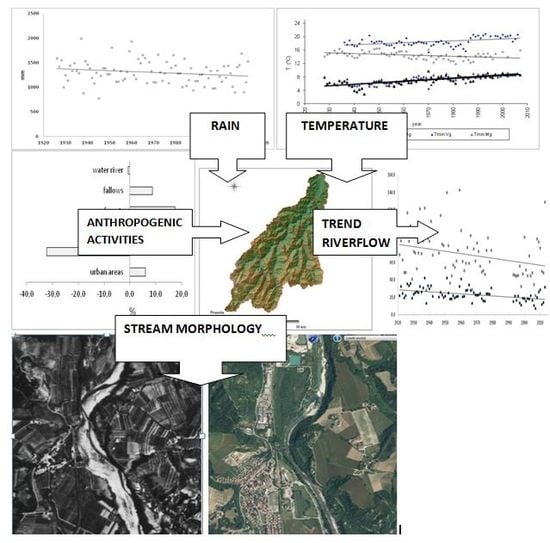
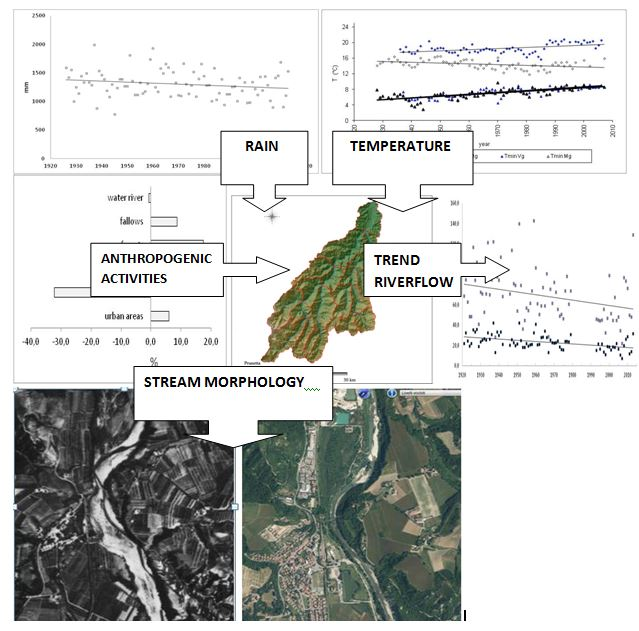
:Anthropogenic activities, and in particular land use/land cover (LULC) changes, have a considerable effect on rivers’ flow rates and their morphologies. A representative example of those changes and resulting impacts on the fluvial environment is the Reno Mountain Basin (RMB), located in Northern Italy. Characterized by forest exploitation and agricultural production until World War II, today the RMB consists predominantly of meadows, forests and uncultivated land, as a result of agricultural land abandonment. This study focuses on the changes of the Reno river’s morphology since the 1950s, with an objective of analyzing the factors that caused and influenced those changes. The factors considered were LULC changes, the Reno river flow rate and suspended sediment yield, and local climate data (precipitation and temperature). It was concluded that LUCL changes caused some important modifications in the riparian corridor, riverbed size, and river flow rate. A 40–80% reduction in the river bed area was observed, vegetation developed in the riparian buffer strips, and the river channel changed from braided to a single channel. The main causes identified are reductions in the river flow rate and suspended sediment yield (−36% and −38%, respectively), while climate change did not have a significant effect.
1. Introduction
The development and specific characteristics of rivers and streams are influenced by surrounding landscapes [1,2]. Our current understanding of rivers’ dynamics incorporates a conceptual framework of spatial nested controlling factors in which climate, geology, and topography at large scales influence geomorphic processes that shape channels at intermediate scales [3]. However, direct human impact on the environment cannot be neglected at a local scale, especially in the last century. In particular, land use/land cover (LULC) changes have a significant impact on basin water cycles and soil erosion dynamics. Human factors also include water abstraction for irrigation, flow regulation, the construction of reservoirs, and mining. An extensive bibliography analyzing the effects of dams and reservoirs on the geomorphic responses of rivers has been produced [4,5,6,7]. However, the influence of other drivers, such as climate and LULC changes has been much less documented over time, although recent studies highlight their importance in inducing river changes [8,9,10,11].
It can be said that agriculture and land abandonment are two complementary aspects of human impacts on the landscape. Land abandonment can affect net soil losses [12], while recolonization of natural vegetation can lead to a reduction in soil loss and a progressive improvement of soil characteristics [13]. Moreover, land abandonment and agriculture can also lead to changes of river stream morphologies, in particular narrowing and incision [13]. Liebault and Piegay [14] observed on the Roubion River (France), that colonization of unstable gravel bars tends to channel minor floods which, in turn, form a new and narrower channel in the existing river bed. A number of studies [3,15] have documented statistical links between LULC and stream conditions, using multisite comparisons and empirical models.
Hydrological alteration is one of the principal environmental factors by which LUCL influences stream ecosystems [3]. It alters the runoff-evapotranspiration balance, can cause an increase or decrease in flow rate’s magnitude and frequency, and often lowers river’s base flow. In addition, hydrological alteration contributes to a change of channel dynamics, including increased erosion of the channel and its surroundings, and a less frequent overbank flooding [3]. Zhang and Schilling [16] noted that increasing streamflow in the Mississippi River was mainly due to an increase in base flow, which in turn was a consequence of LULC (conversion of perennial vegetation to seasonal row crops). Many researchers have studied the effects of LULC changes on river flow and most of them have indicated that intensified afforestation will reduce both runoff peak and total runoff volume [17]. On the other hand, even a modest riparian deforestation in highly forested catchments can result in the degradation of a stream habitat, owing to sedimentary input. A comparison of different catchments showed that an increased forest area results in lower concentrations of suspended sediments, inferior turbidity at base flow, lower bed-load transport, and less embeddedness [3].
Numerous studies have demonstrated that LULC, the abandonment of rural activities, and consequently, a decrease of human pressure on mountain areas, has contributed to increase of vegetation cover [18,19,20]. In the case of Reno River mountain basin, Pavanelli et al. [21] documented that recolonization of natural vegetation and a consequent increase of actual evapotranspiration, was the key hydrological variable that caused the decrease of the river flow rate. However, not many studies have addressed the effect of the redevelopment of natural vegetation at the river-basin scale on river flow, sediment yield, and riverbed morphology. Picco et al. [22] noted a consistent increase of riparian vegetation within the corridor of the Piave River (Northern Italy) during the last five decades, concluding that it depended on human activities, both in the main channel and at basin scale. LULC and local climate change (e.g., precipitation, temperature and evapotranspiration), may induce notable alterations of watershed hydrology [13,23]. Several studies showed that precipitation increase alone is insufficient to explain increasing flow rate trends in agricultural watersheds [24,25], since changes in agricultural land use can also result in increased flow rate.
Collectively, these studies provide strong evidence for the importance of the surrounding landscape, and human activities for the hydrological and morphological characteristics of rivers [3,15]. However, it is often difficult to separate human from naturally driven activities [26]. In addition, most of these articles were mainly conducted on small spatial scales, within a few hundred meters of a stream, without considering larger spatial units. Finally, only few studies have addressed the effect of redevelopment of natural vegetation at the river basin scale on river discharge, sediment yield, and bed river morphology.
Therefore, the aim of this paper was to explore relationships between local climate change that occurred in the last century and agricultural land abandonment (and consequent LULC changes), which culminated in the 1950s, on the one hand; and modifications in morphology and hydrology of the Reno River (Northern Italy), on the other hand.
2. Materials and Methods
2.1. Study Area
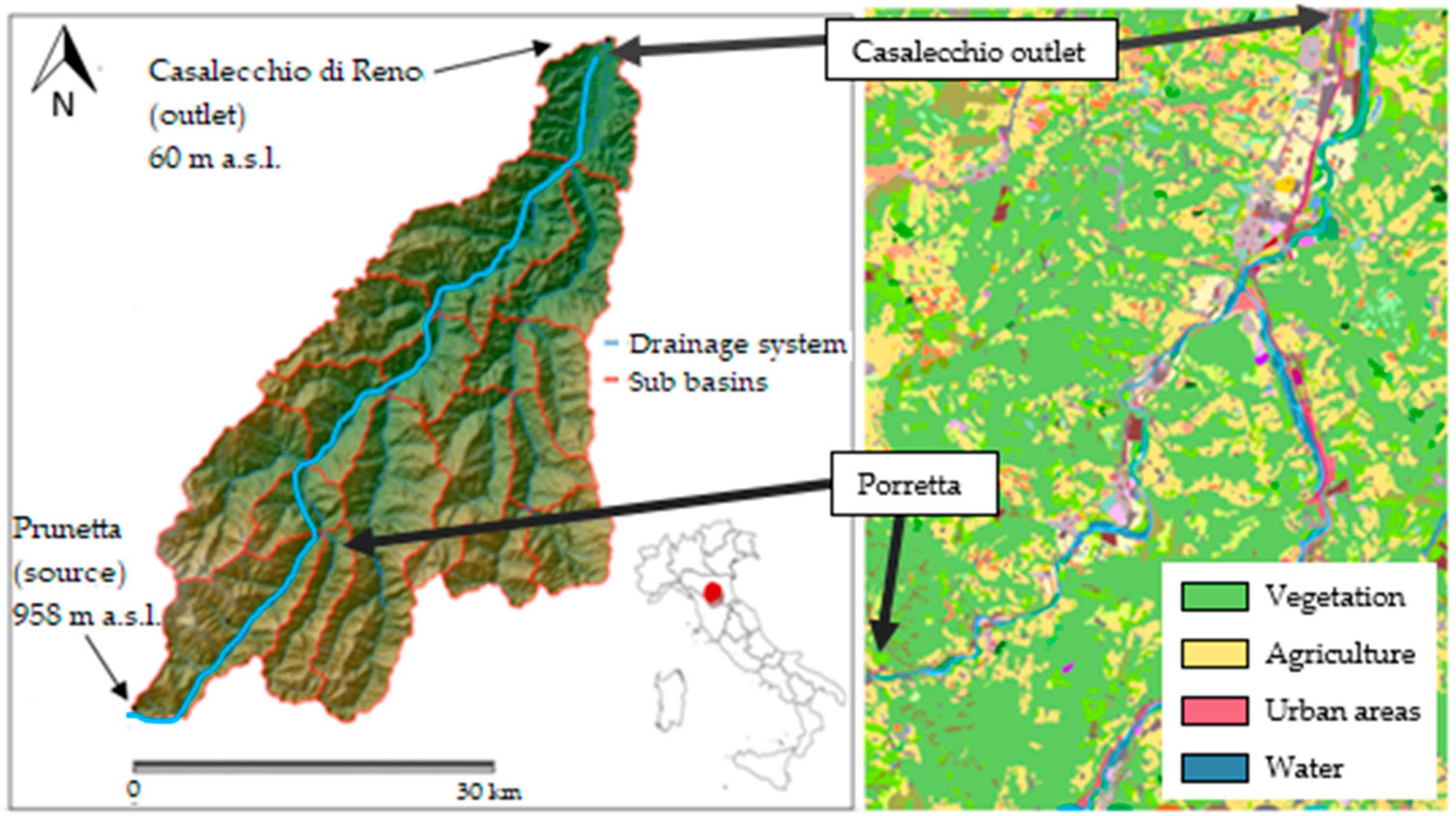
The Reno River, located in the Northern Italy, flows into the Adriatic Sea. It is the sixth biggest Italian river, with a catchment area of 5965 km2 and a length of 211.8 km. The mountain hydrographic network of the Reno is rather ramified and dense, and it is composed of eight major rivers, 12 secondary rivers and 600 torrents. This study concentrates on one part of the Reno River; namely, the Reno River Mountain Basin (RMB), located in the Northern Italian Apennines (Emilia Romagna and Tuscany Regions), with a catchment area of 1061 km2 and length of 80 km. The RMB’s average altitude is of 639 m a.s.l.; it ranges from a maximum elevation of 1945 to a minimum one of 60.35 m a.s.l. at the dam of Chiusa of Casalecchio (44°47’ N, 11°28’ E), which is the RMB outlet (Figure 1).
The RMB can be considered representative of the environmental and anthropogenic changes that have occurred in the Italian central and northern Apennines in the last century. The Apennine agricultural area of the Emilia Romagna Region (RER) decreased by almost 50% from 1960 to 2000 [27]. After 1950, the population moved to the cities and valley, a phenomenon that affected the whole Italian Apennines. Until World War II, this area had an average population density of 85 inhabitants km−2, with agro-forestry and pastoral farming as the main activities. Currently the density is reduced to less than 70% of the previous one [27]. After World War II, due to industrialization and the development of agricultural mechanization, the landscape rapidly transformed. Agriculture remained where it was cost-effective, while the rest gave way to permanent meadows, scrub, and woodland [28]. Currently, land cover is characterized by oak woods, beeches, shrubs, and pastures at higher altitudes. Chestnut woods are present at medium altitudes and on coppices, pastures, and crops on hillsides. Crops, vineyards, orchards and urban areas cover the catchment valley (Figure 1).
The RMB consists mainly of erodible sedimentary rocks. Land cover, runoff, soil erosion, and suspended sediment in the river are closely related to each other. The bedrock consists of resistant limestone, sandstone, and meta-sandstone in the upper part of the watershed and of weakly cemented marl, mudstone, sandstone, and conglomerate in the middle and lower part of the watershed [29]. The fluvial terraces are preserved from the outlet (Casalecchio) to about 20 km upstream (~150 m a.s.l.). Upstream of that point, landslides and earthflows preclude significant preservation of terraces.
The RMB average precipitation is 1305 mm year−1 (Table 1), with the following distribution: Winter 337 mm, spring 307 mm, summer 182 mm, and autumn 411 mm. The average temperature is 10.7 °C; July is the hottest month, with peaks up to 29.5 °C (1998). Winters are generally very cold, with the average minimum monthly temperature dropping to −8.9 °C (January 1942). The fluvial regime of the Reno River is linked to rainfall, with floods occurring in autumn and spring. Seasonal floods are characterized by short times of concentration (time it takes to reach the basin outlet), owing to the long and narrow shape of the catchment. The evaluations of the 30 and 200-year recurrence interval floods at Casalecchio (Chiusa) are 1541 and 2280 m3 s−1, respectively.
The dam “Chiusa of Casalecchio” is the RMB outlet. It is the oldest hydraulic building in Europe, and has allowed the social and economic development of the city of Bologna through hydraulic energy since the XII century. It is also included in the UNESCO program’s list of Patrimony Messengers of a Culture of Peace. The Chiusa dam controls the downstream base level, making the reach from the source to the Chiusa geomorphologically independent. Census of the hydraulic works detected 51 weirs on that reach, and most of them were built in the first decades of the 20th century. Similarly, in Rio Maggiore, a tributary of Reno, there is a total of 162 dams, which equals a 10 dam km−2 density [28]. Moreover, in the early 1900s, five hydroelectric dams were built in the tributaries of the Reno. Even though dams and reservoirs do not influence river water budget on the longer time scale, they do act as river sediment traps and can affect the river flood regulation [21]. During the last few decades, part of water has been diverted for domestic and irrigation purposes; however, these withdrawals represent a very limited percentage (3%) of the Reno river’s flow rate [21].
2.2. Methodology
The parameters considered in this study were LULC (since the 1950s), river morphology (in 1954 and 2003), and hydro-climate changes (since the 1920s) of the RMB. They were used to assess different environmental changes that occurred in the RMB and whether if they were due to agricultural land abandonment and a consequent renaturalization after the 1950s. The main hypothesis of this research is that the year 1960 is the date from which effects of these changes can actually be seen.
2.2.1. Land Use Changes
As already said, the year 1960 was taken as a point when effects of big LULC changes started to be visible, and the year 1954 was taken as representative of the period before agricultural land abandonment. The two LULC maps are both to the scale 1:25000 (Soil Use Maps RER 1954 and 2003) were derived from the black and white aerial photographs flight G.A.I. 1954 (Military Geographic Institute-Italy) and the satellite images from 2003 (Quickbird). They were analyzed and compared with Geographic Information System software ARCVIEW 3.2 (Environmental Systems Research Institute, Redlands, CA, USA) to evaluate the RMB LULC changes. The relatively heterogeneous classes of the two different maps were reclassified according to the CORINE land cover classes [30] in order to be compared. Then, 20 and 51 land cover classes of the 1954 and 2003 Soil Use Maps respectively, were grouped into urban areas, water bodies, fallows, forests, and crops. This approach reduced the error due to the different sources of images of the maps. In Figure 1 fallows and forests are grouped together to highlight natural vegetation and renaturalization effects.
2.2.2. Morphological River Changes
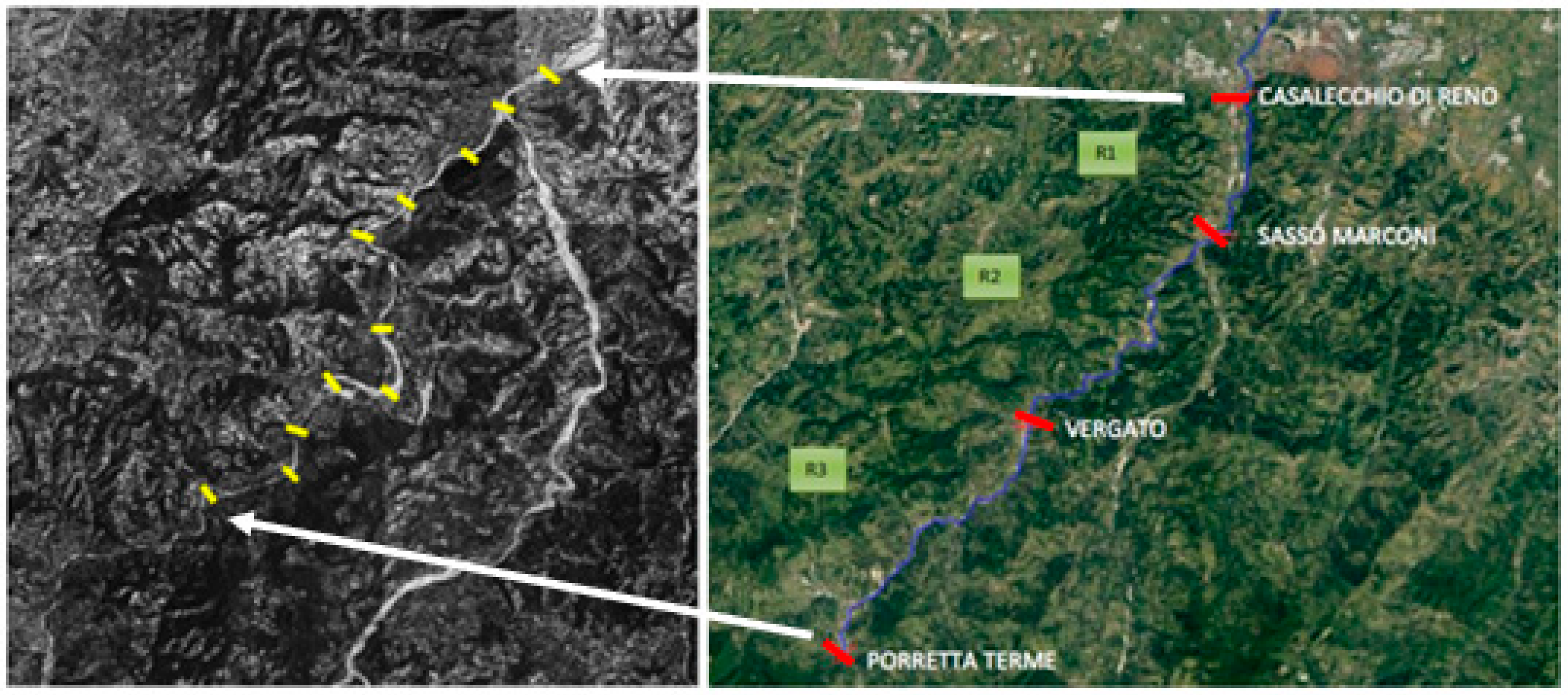
To assess changes to the river belt and river morphology, aerial photos from the year 1954 (GAI-IGMI) and satellite images from Quickbird, 2003 (Figure 2), were used. The effects of LULC changes and human impact on the Reno river terraces and banks were analyzed on a reach from Porretta Terme (349 m a.s.l.) to Casalecchio di Reno (60 m a.s.l.), with a length of 54.5 km and a mean bed river slope of 0.53%. The area was within 250 meters from each side of the river bed, done using GIS software. The transects (Figure 2 left) were drawn using the same reference points for both 1954 and 2003, to estimate variations in the river bank width, vegetation, and stream bed. The river’s morphological changes, the width, the river’s channel area, and the riparian LULC of each transect, were evaluated. The river channel was identified in the images as a non-vegetated part of river bed corresponding to the physical confine of the normal water flow. Banks, on the other hand, are subject to water flow only during high water stages and a riparian buffer strip is the vegetated area near a stream. All of them constitute the river corridor.
The studied 54.5 km portion of the Reno river was split into three reaches (Figure 2, right), on the basis of similar morphological characteristics (mean width and slope of the river and its banks): R1 from Porretta Terme to Vergato (21 km long), R2 from Vergato to Sasso Marconi (23 km long) and R3 from Sasso Marconi to Casalecchio Chiusa (10.5 km long). The properties of the three reaches were obtained from field survey of the transects and from the 1954 and 2003 images. The cartographic and photo-interpretation data were managed with GIS ARCVIEW 3.2 software used for map drawing and calculating the extent of the areas covered by vegetation. On the other hand, data on the river morphology (e.g., type of riverbed material) and vegetation type in the transects were obtained during field surveys.
2.2.3. Climate and Hydrological Data
The Reno River hydrological and RMB climate data (Table 1), were processed on a monthly, yearly and seasonal basis, and they were divided into two periods—before and after 1960, the year that was taken as a date from which effects of LULC changes and renaturalization can be seen. The monthly data of the river flow rate (Q) and the suspended sediment yields (SSY) are came from samples collected at the outlet of the RMB (Casalecchio di Reno gauge, 60 m a.s.l.) by the Italian Hydrographical Service (SIMI) and by the Regional Agency for Environmental Protection of the Emilia Romagna Region (ARPAE).
In addition, precipitation and temperature data collected by the SIMI and ARPAE were analyzed to evaluate impact of climate change on the RMB. For the minimum and maximum monthly temperatures of the two RMB stations: One in the mountains (Monteombraro, at 704 m. a.s.l.) and one in the valley (Anzola at 42 m. a.s.l.) were examined (Table 1).
2.2.4. Data Analysis
Statistical analyses were performed on the data records with the STATGRAPHICS® Centurion XVI software (StatPoint Technologies, Inc., The Plains, VA, USA). Statistical tests were used to verify whether the river flow rate data (Qmean and Qmax) detected before 1960 (1921–1959) were statistically different from the data collected after 1960 (1960–2013). Two samples were compared using F test, discriminant analysis, box and whisker plots, t-tests, the Kolmogorov–Smirnov Test, and analysis of variance tests. Discriminant analysis was run on flow rate samples to verify if each value was correctly classified in the two periods. The t-tests were run to compare means of the two samples and to test the null hypothesis that the two means were equal. The results were verified with a Kolmogorov–Smirnov test and the distributions of the two samples were compared, for both the Qmean and the Qmax. Finally, a box and whisker plot was run to demonstrate a significant difference (p < 0.05) between the flow rate data coming from the two periods considered.
Moreover, the river flow rate, SSY and climate data were also analyzed with linear trend analysis in order to show linear regression in the examined periods with 95% confidence limits and the prediction limits of the least squares fit model. Trend-line slopes (b) were calculated by the least-square linear fitting method.
3. Results and Discussion
3.1. LULC Changes
At present, more than 60% of the entire mountain Reno catchment is covered with forest [31], while in the past, forest was scarce due to exploitation (Figure 3). Cultivated land in the RMB catchment decreased from about 37% in 1954 to 5% in 2003, partially losing space to forest, which is, in fact, mainly 50–60 years old (Figure 4). In detail, forests and fallows increased from 39.5% to 57% and from 19% to 28%, respectively. Urban areas increased from 0.45% (1954) to 6.5% (2003), with the majority of population concentrated in the Reno valley. Lastly, water surfaces were found to be 40% smaller—they reduced from 9.3 km2 in 1954 to 5.7 km2 in 2003 (Figure 4a). The disappearance of rocky outcrops that were predominantly clayey badlands, the so called “Calanchi,” is also interesting: They decreased from 1.67% to 0.46% of the RMB area, a phenomenon that was repeated throughout the Apennines.
LULC changes noted in the riparian buffer strips between 1954 and 2003 were an increase of forests, urban areas, and uncultivated land, at the expense of cultivated land (that decreased from 60.25% to 11%) (Figure 4b). That decrease was the most prominent near the city of Bologna (reach R3, Figure 2), where cultivated land decreased from 85% (1954) to 20% (2003), while urban areas and woods showed an increase, from 7% to 42%, and from 8% to 38%, respectively.
The most widespread species (40–50%) in the riparian buffer strips are Populus nigra and Salix alba. Besides them, other species present are Quercus pubescens (about 20%) and Salix alba (10–15%), that form mixed populations, and different arboreal and shrub forms. Alnus glutinosa (about 10%) is present in the upper river banks where the anthropic impact is less. The shrub layer is composed of Sambucus nigra, Corylus avellana, Cornus sanguinea, and Prunus spinosa. Exotic species that have found, in this fluvial habitat, the ideal conditions of development, are Robinia pseudoacacia and Acer negundo, while among the shrubby, an infesting species is Amorpha fruticose.
3.2. Hydrology Changes
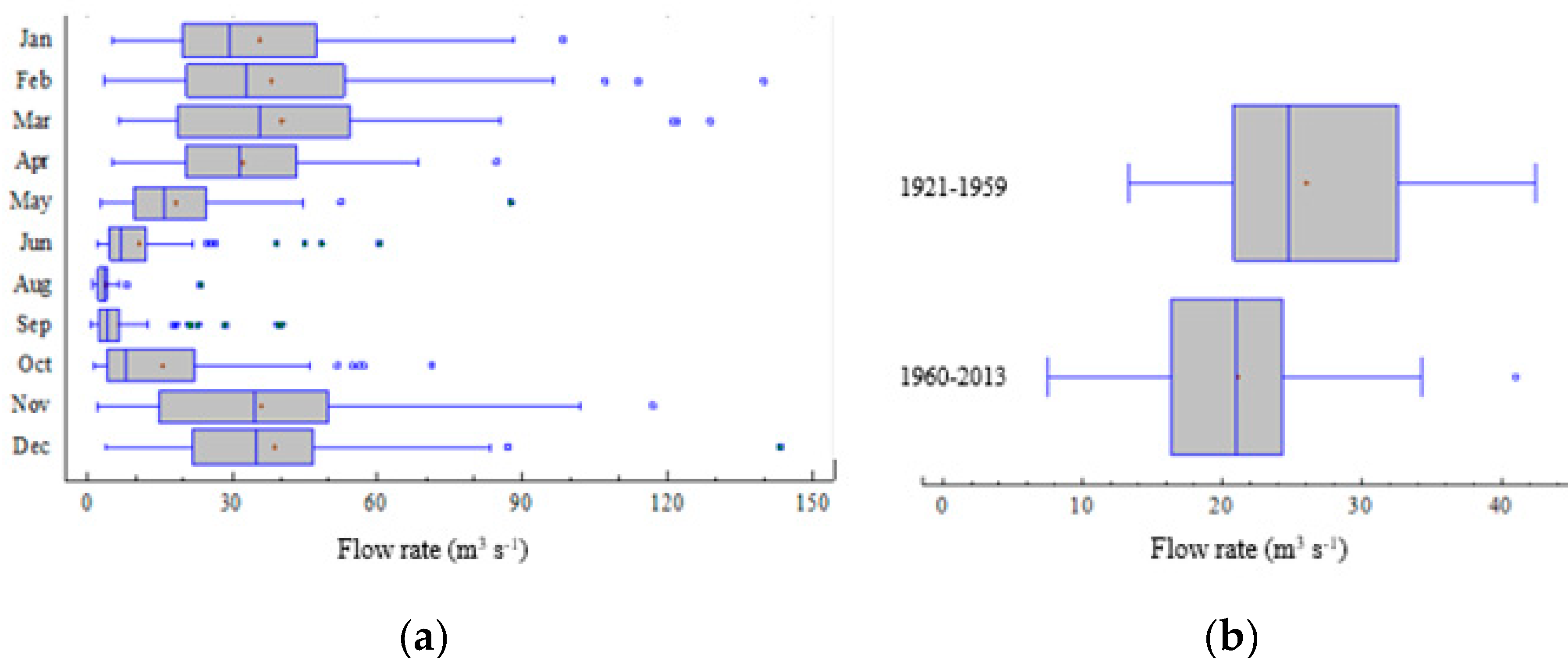
The monthly mean flow rate of the Reno River is 23.4 m3 s−1, while the maximum monthly value recorded was 143 m3 s−1 in December 1959 (Table 2). Between 1921 and 2013, the mean yearly flow rate was reduced by 11 m3 s−1 (b = −0.12) or 36% (Figure 5), while the Qmax reduction was about 30.3%. The correlation coefficient (R2) values of linear regression for Qmean and Qmax were 0.22 and 0.08, respectively. Since the p-values were both less than 0.05, there was a statistically significant relationship at 95% confidence level. The monthly flow rate values are given in the box and whisker plot (Figure 6a). Starting from the hypothesis that the renaturalization and consequent hydrological changes caused by agricultural land abandonment in the 1950s were detectable after 1960, river flow rate data was divided into two sub-periods: Before and after this date. The Qmean values were 26.03 m3 s−1 and 21.08 m3 s−1, for the 1921–1959 and 1960–2013 periods, respectively (Figure 6b). The F-test and p-value were, respectively, equal to 9.79 and 0.0026, according to the ANOVA test. Since the p-value was less than 0.05, there was a statistically significant difference between the two flow rate means.
Discriminant analysis was run on the two groups of Qmean: Before and after 1960. From the 77 values used to fit the model, 72.7% were correctly classified in the groups, out of which 66.7% and 78% were for 1921–1959 and 1960–2013, respectively. A statistically significant difference (p < 0.05) was found between the two groups, for both Qmean and Qmax (Figure 6b). It was evident that the lowest flow rate values were mostly concentrated during the 1960-–2013 sub-period. In fact, there was a marked change in the trend of Qmax and Qmean around 1960. Additionally, significant differences between the two periods were shown by discriminant analysis, as dispersion and as data trend. Dispersion of the mean flow rate data for the first period (1921–1959) was higher in respect to the second one (1960–2013), as evidenced by correlation coefficients R2 (0.04 and 0.20 respectively), and therefore the two groups are statistically different. This difference, particularly the higher value of dispersion data of the first period, indicated presence of floods events, including disastrous ones [30].
3.3. Suspended Sediment Yield (SSY)
LULC change is an important factor that affects soil erosion-runoff and SSY. The relationships between climate and LULC changes on one side and SSY on the other, was investigated by PJ Ward et al. [32], with use of geo-referenced model WATEM/sedem. The authors found that the sediment increase in the Meuse, a northern European river, was almost entirely due to LULC change (conversion of forests to agricultural land). They concluded that increase of riparian buffer strip and development of riparian vegetation can result in the reduction in SSY, as they can be used as barrier to soil runoff [33].
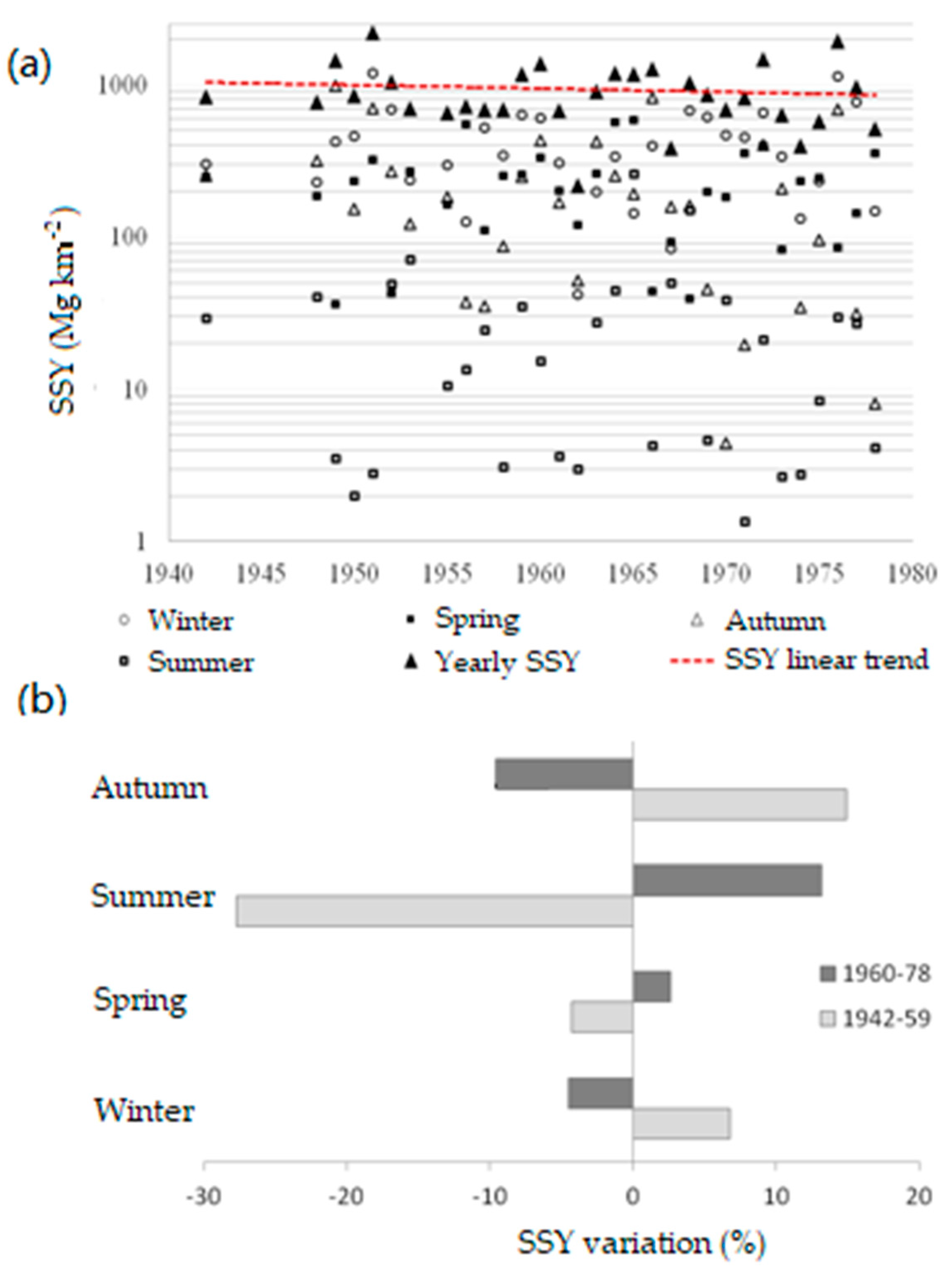
Similarly, in the Apennines, SSY can be used to assess a real loss of the catchment soil due to runoff, rills erosion, gullies, and badlands, but also losses due to agricultural land abandonment and LULC change [33,34]. Currently, soil erosion prevails in the badlands and agricultural areas that are concentrated on the slopes, and that are easily accessible to mechanization. The average yearly SSY in the period 1942–1978 was 934.3 Mg km−2. The maximum monthly value was 960 Mg km−2 in December 1976 and the yearly maximum value was 2225 Mg km−2 in 1951 (Table 2). Yearly and seasonal SSYs are given in the Figure 7a. It can be seen that the analysis of the SSY linear trend indicated a 17.5% reduction during the year 31 of data, or a 38% reduction in the period 1921–2013.
For the period 1942-1978, the seasonal SSY averages were: 426 Mg km−2 (winter), 231 Mg km−2 (spring), 32 Mg km−2 (summer) and 244 Mg km−2 (autumn) (Figure 7a). The average SSYs for the two sub-periods 1942–1959 and 1960–1978 (Figure 7b) were 981 and 902 Mg km−2 respectively. Moreover, some interesting seasonal variations occurred. For example, compared to the 1942–1978 seasonal average, SSY in the second period was lower in winter and autumn (−4.5% and −9.6%, respectively). On the other hand, it increased in spring and summer by 2.6% and 13.2% respectively (Figure 7b).
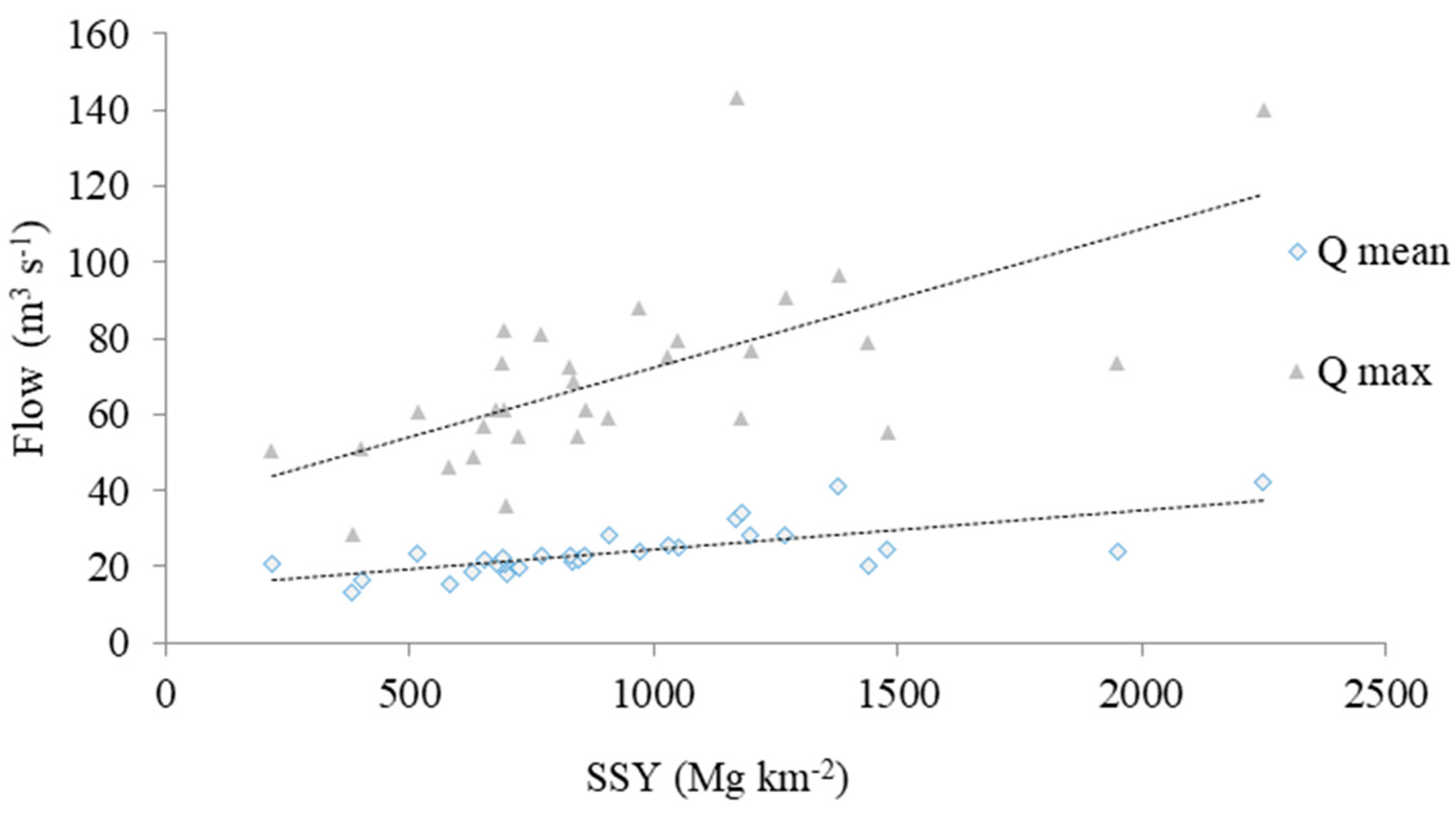
In general, the highest average monthly values of SSY were in February and November (213 and 188 Mg km−2, respectively), but they decreased by 37% and 32% in the two following decades. If seasons of the two periods are compared, it can be noted that SSY reduced in summer and spring, while it increased in winter and autumn (Figure 7b). Finally, linear relations between the yearly SSY and Qmean and Qmax, showed that SSY is better correlated to the maximum flow rate (Figure 8).
The average annual erosion in the RMB, calculated on the basis of 31 year of SSY data, was about 9.3 Mg ha−1 year−1 or 0.6 mm year−1. Various bibliography estimates available for the Region of Emilia Romagna give different results. The European Agency for the Environment, using the model Pesera [35], estimated a soil loss of 2.42 Mg ha−1 year−1, slightly below the average Italian value (3.11 Mg ha−1 year−1). In addition, the Emilia Romagna Region (including the RMB) was defined as a soil erosion risk area [36]. It was found that around 21% of the region has a medium to high risk of soil loss. The average loss in higher grounds of the region was estimated to be around 6 Mg ha−1 year−1 [37]. The difference between the erosion value reported in this study and other researchers’ ones is mainly due to the heterogeneity of estimation models and basic data being estimated. Considering the current conditions of vegetation cover, they are all lower than those calculated on the basis of historical data from the 1942–1978 period.
3.4. Climate Change
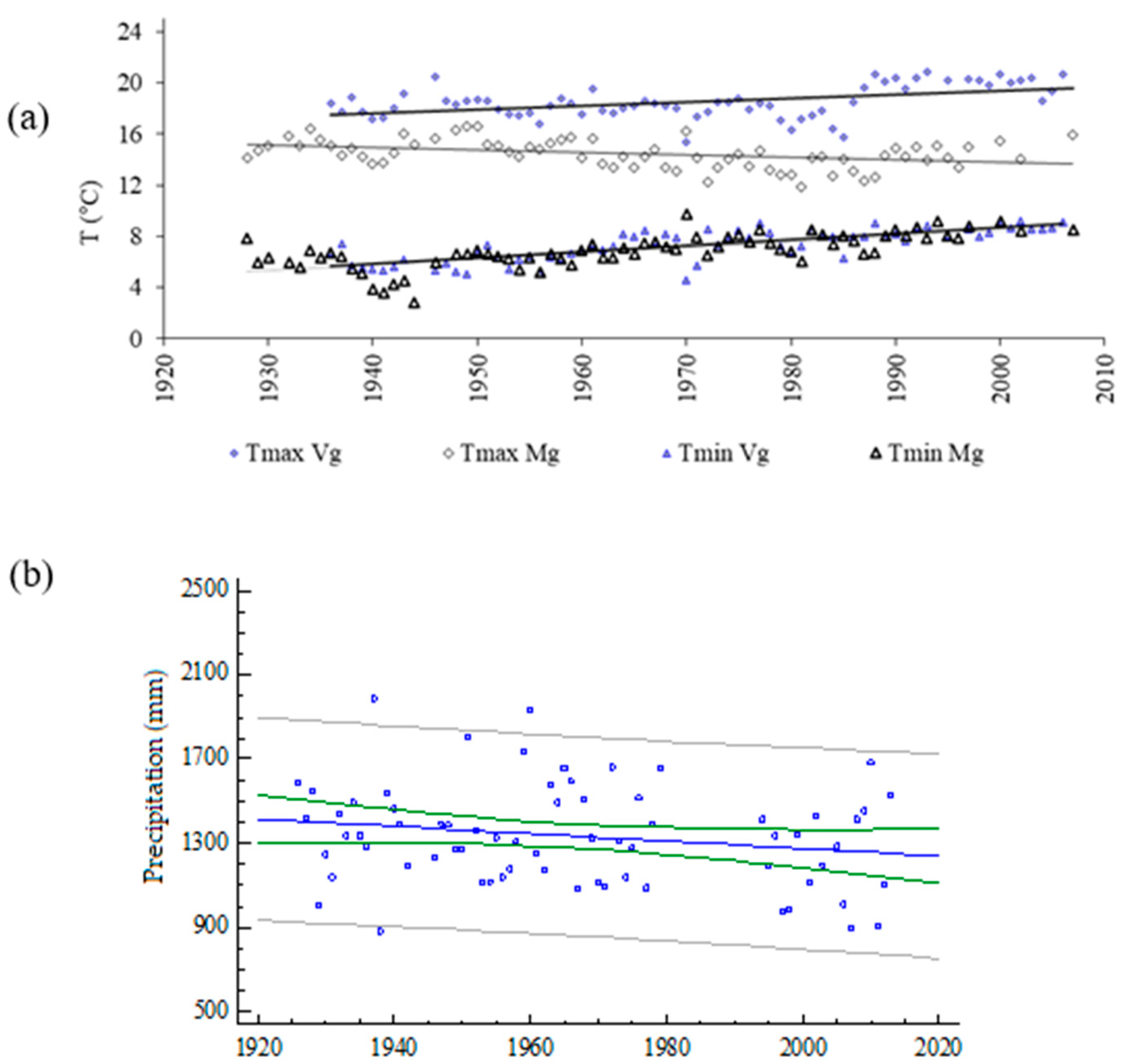
An important aspect of a basin water budget is climate: Temperature and precipitation trends. In fact, temperature variations influence hydrology and river flow rate, and since they have an impact on evapotranspiration from vegetation, water surfaces and soil. Figure 9a shows a linear increase for both minimum and maximum mean yearly temperature in the RMB. That is visible for the mountain and valley gauge. The minimum temperature (Tmin) showed a similar rising trend for the two stations: +4 °C/100 years (R2 = 0.49) for the Mountain gauge and +5 °C/100 years (R2 = 0.59) for the Valley gauge. On the other hand, Tmax trends were more complex—decreasing in the mountain areas (−1.9 °C/100 years; R2 = 0.15) and showing an increase in the valley (+2.8 °C/100 years; R2 = 0.21). Since only the minimum, hence night, temperatures increased in the mountain areas where vegetation is also more developed than in the valley, and since night-time evapotranspiration is much smaller than in the day-time, the temperature increase most probably did not have a big influence on the observed flow rate reduction.
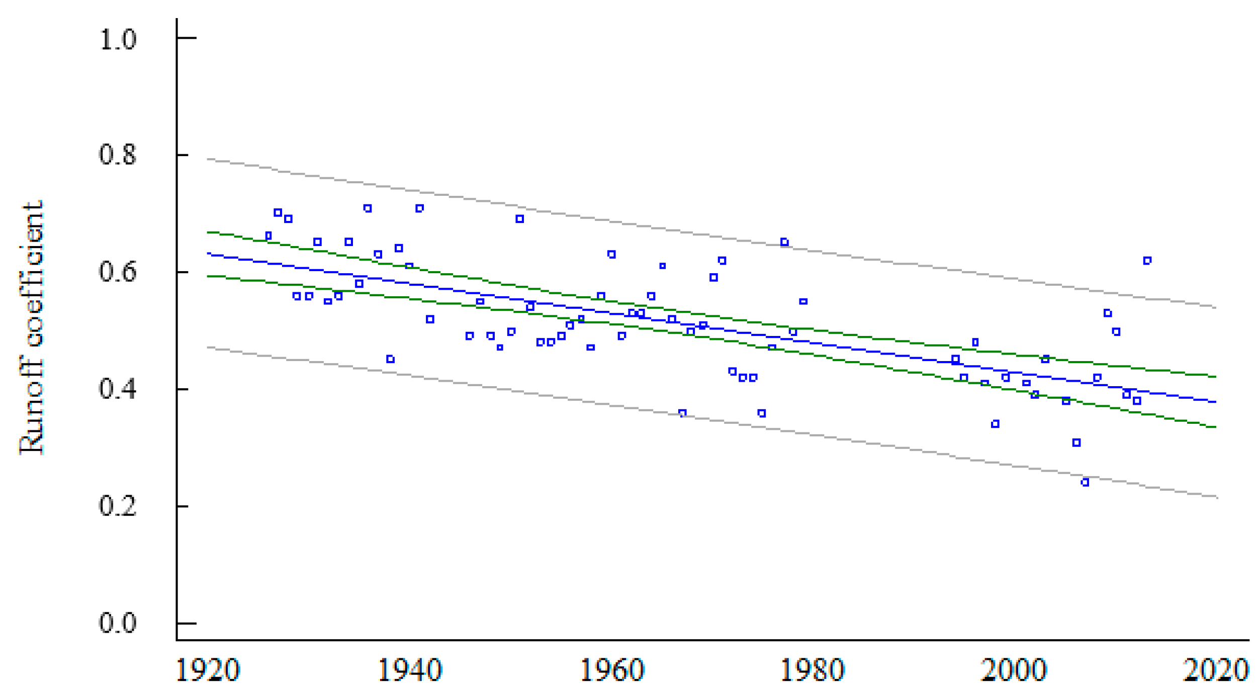
Precipitation in the RMB was lowered by 10.67% between 1921 and 2013 (Figure 9b), corresponding to 145 mm reduction in 92 years. However, that value is not statistically significant (R2 = 0.034). A strong reduction (from about 0.6 to 0.4) in the catchment runoff coefficient (flow rate/precipitation), that was observed in the last 90 years (R2 = 0.43) (Figure 10), and is mainly due to reduction of the flow rate.
3.5. Morphological Stream Changes: Riparian Buffer Strips
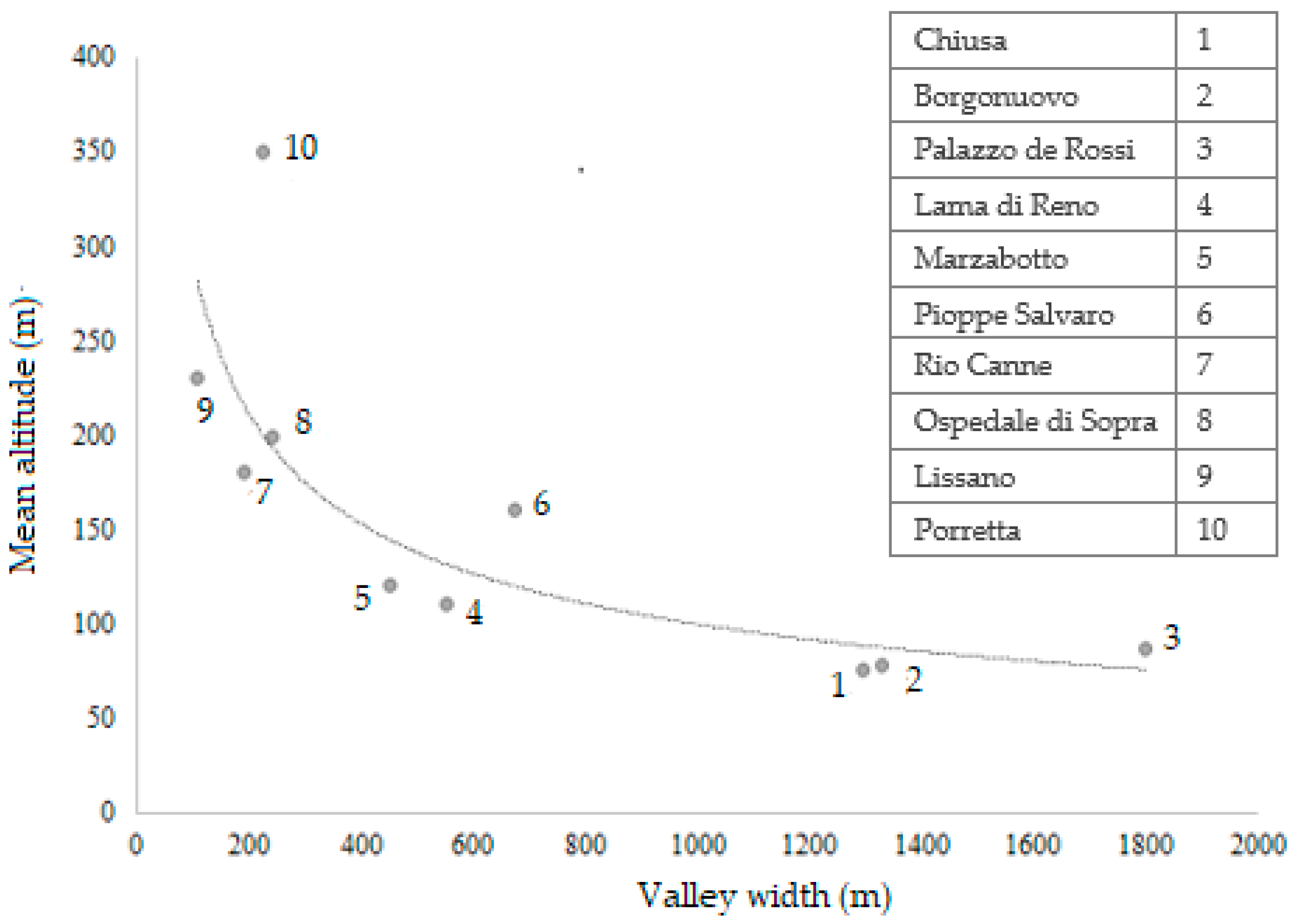
The main proprieties and changes of the three reaches considered, based on aerial and satellite images, and field surveys, are reported in Table 3. Figure 11 gives the relationship (exponential equation, R2 = 0.75) between the average width and mean altitude of the Reno valley. The two values that are above the curve are of two villages (Porretta and Pioppe di Salvaro) that are in a larger area due to tributary torrents. The changes of the Reno River reaches (R1–R3) concern the banks and the river morphology (Figure 12), from upstream to downstream:
- R1 is a more torrential reach of the river; the valley is narrower and currently characterized by woods and meadows. The normal riverbed flow occupied 210 ha in 1954, but it reduced to 80 ha in 2003 (Table 3). It was and is predominantly covered by gravel pits, sand deposits, and rock outcrops. Riparian forests currently cover an overall surface of 53.8 ha (Figure 12), while in 1954 they were absent due to farming activities.
- R2 is the middle reach. Its normal flow riverbed in 1954 occupied 206 hectares, and it was predominantly made of gravel pits and sand deposits. Instead, in 2003, the area occupied by the riverbed reduced to 78 ha (Table 3). On stabilized alluvial deposits of the river stream, where occasional floods occur, there are typical igrophilous-forests, consisting of elms, poplars, and willows (Figure 13).
- R3 is a fluvial stretch in which the valley widens and then turns to the Po Valley. The riverbed area decreased from 299 ha to 61 ha between 1954 and 2003 (Table 3). In 1954 the riverbed consisted of gravel bars and sand deposits, while currently clay and silt prevail. In addition, the river channel changed from braided to a single one. Riparian forest showed a strong development: it was discontinuous in 1954 and inadequate as a buffer zone, while currently it is well developed and forms a continuous wooded area (Figure 12). The fluvial park and most of riparian forests are now protected by the EU Habitats Directive (Habitat Code 92A0).
Based on the RMB’s soil use maps, it was estimated that the riverbed area decreased by about 40% from 1954 to 2003. However, based on the river transects, the reduction was as high as 80%. Fluvial banks with woods along the Reno were mostly absent in 1954, and the area was used for farming. In 2003 riparian forests appear to be well developed along the entire stream in the RMB. This is especially visible on the right-hand side (looking downstream) of the river, where fluvial terraces are narrower or absent, and are therefore under a lower human impact. In general, it is observed that the river bed gives way to riparian forests. For example, a reduction in the active riverbed corresponds to formation and/or expansion of the riparian buffer strips, and the stream reaches are colonized by riparian vegetation.
4. Conclusions
This study has examined relationships between two major geomorphological changes (channel narrowing and formation of wide vegetated banks) that took place in the Reno River mountain basin in the last century, and the hydrological, climatic, and basin re-naturalization factors that have contributed to these changes. The two phenomena are strongly and positively covariant, indicative of cause and effect, and in fact, wide vegetated banks are formed at the expense of the riverbed. While riparian buffer strips were mostly absent in 1954, currently they are well developed along the entire stream. In addition, the shape of the river channel changed from braided to a single one and the width of the river bed was reduced by around 80%. The riverbed in the past, mostly consisted of gravel bars and sand deposits, and currently clay and silt prevail at the basin outlet.
Based on this study, the steering factors for those changes and significant aspects were:
- LUCL changes between 1954 and 2003: A reduction in the agricultural land use (from 37 to 5%), an increase of forest cover (from 40% to 57%), and development of riparian vegetation.
- Considerable reduction in SSY (−38%) and flow rate (−36%) during the last 90 years, and a consequent change of runoff coefficient (reduction from about 0.6 to 0.4), was an important parameter for hydraulic watershed management.
The effect of agricultural land abandonment that occurred in the 1950s can be recognized after 1960, confirming the initial hypothesis that this year can be taken as a starting point for the basin change. After that date a decrease in the Reno flow rate was observed and dispersion of data is significantly reduced. All statistical analyses confirm that the hydrological flow data measured after 1960 (period 1960 to 2013) are significantly different from those measured when the basin was still heavily agricultural (period 1921 to 1958). However, although this study has identified the human factor as one of the main causes of the above-mentioned changes, it can often be challenging to separate human from naturally driven activities, and future research is needed in order to do it. The geomorphological evolution of the Reno River shows how these changes are mainly related to the hydrological dynamics and catchment re-naturalization. Although climate changed in the period studied (precipitation reduction of 10.67% and 4–5 °C increase of Tmin) it had little bearing on the observed environmental changes.
This study, applied to a typical North Apennine river, illustrates the effectiveness of combining historical data (hydrological and climate data, so as aerial and satellite images) on the one hand, and the use of modern technology (geographic information systems) and direct surveys on the other. Combining these techniques can certainly contribute to a sustainable management of river systems. Although further research is needed, this study gives an insight to the past and present factors that regulate water course, its hydrology, and morphology. An in-depth knowledge of this factors can certainly make it possible to predict the evolution and dynamics of the Reno river flow and its morphology.
Author Contributions
Conceptualization, D.P.; methodology, D.P. and C.C.; validation, D.P.; formal analysis, D.P.; data curation, D.P. and C.C.; writing—original draft preparation, D.P.; writing—reviewing and editing, D.P., S.L., and A.T.; visualization, D.P. and S.L.; supervision, D.P. and A.T.
Funding
This research received no external funding.
Acknowledgments
This research was undertaken as part of the collaboration agreement for teaching and study with the Emilia Romagna Region, Civil Protection, Basin Authority of the Reno River and ARPAE-RER, (Italy).
Conflicts of Interest
The authors declare no conflict of interest.
References
- Hynes, H.B.N. The stream and its valley. Verh. Internat. Verein. Limnol. 1975, 19, 1–15. [Google Scholar] [CrossRef]
- Vannote, R.L.; Minshall, W.G.; Cummins, K.W.; Sedell, J.R.; Cushing, C.E. The river continuum concept. Can. J. Fish. Aquat. Sci. 1980, 37, 130–137. [Google Scholar] [CrossRef]
- Allan, J.D. Landscapes and riverscapes: The influence of land use on stream ecosystems. Annu. Rev. Ecol. Evol. Syst. 2004, 35, 257–284. [Google Scholar] [CrossRef]
- Graf, W.L. Downstream hydrologic and geomorphic effects of large dams on American rivers. Geomorphology 2006, 79, 336–360. [Google Scholar] [CrossRef]
- Schmidt, J.C.; Wilcock, P.R. Metrics for assessing the downstream effects of dams. Water Resour. Res. 2008, 44, W04404. [Google Scholar] [CrossRef]
- Burke, M.; Jorde, K.; Buffington, J.M. Application of a hierarchical framework for assessing environmental impacts of dam operation: Changes in stream flow, bed mobility and recruitment of riparian trees in a western North American river. J. Environ. Manag. 2009, 90, S224–S236. [Google Scholar] [CrossRef]
- Martínez-Fernández, V.; Maroto, J.; García de Jalón, D. Fluvial corridor changes over time in regulated and nonregulated rivers (Upper Esla River, NW Spain). River Res. Appl. 2017, 33, 214–223. [Google Scholar] [CrossRef]
- Piégay, H.; Walling, D.E.; Landon, N.; He, Q.; Liébault, F.; Petiot, R. Contemporary changes in sediment yield in an alpine montane basin due to afforestation (the upper Drôme in France). Catena 2004, 55, 183–212. [Google Scholar] [CrossRef]
- Keestra, S.D.; Van Huissteden, J.; Vandenberghe, J.; Ol, V.D.; De Gier, J.; Pleizier, I.D. Evolution of the morphology of the river Dragonja (SW Slovenia) due to land-use changes. Geomorphology 2005, 69, 191–207. [Google Scholar] [CrossRef]
- Pont, D.; Piégay, H.; Farinetti, A.; Allain, S.; Landon, N.; Liébault, F.; Dumont, B.; Richard-Mazet, A. Conceptual framework and interdisciplinary approach for the sustainable management of gravel-bed rivers: The case of the Drôme River basin (S.E. France). Aquat. Sci. 2009, 71, 356–370. [Google Scholar] [CrossRef]
- Piqué, G.; Batalla, R.J.; Sabater, S. Hydrological characterization of dammed rivers in the NW Mediterranean region. Hydrol. Process. 2015, 30, 1691–1707. [Google Scholar] [CrossRef]
- Debolini, M.; Schoorl, J.M.; Temme, A.; Galli, M.; Bonari, E. Changes in agricultural land use affecting future soil redistribution patterns: a case study in Southern Tuscany (Italy). Land Degrad. Dev. 2013, 26, 574–586. [Google Scholar] [CrossRef]
- García-Ruiz, J.M.; Lana-Renault, N. Hydrological and erosive consequences of farmland abandonment in Europe, with special reference to the Mediterranean region, a review. Agric. Ecosyst. Environ. 2011, 140, 317–338. [Google Scholar] [CrossRef]
- Liébault, F.; Piégay, H. Causes of 20th century channel narrowing in mountain and piedmont rivers of southeastern France. Earth Surf. Process. Landf. 2002, 227, 425–444. [Google Scholar] [CrossRef]
- Tomer, M.D.; Schilling, K.E. A simple approach to distinguish land-use and climate-change effects on watershed hydrology. J. Hydrol. 2009, 376, 24–33. [Google Scholar] [CrossRef]
- Zhang, Y.K.; Schilling, K.E. Increasing streamflow and baseflow in Mississippi River since the 1940s: Effect of land use change. J. Hydrol. 2006, 324, 412–422. [Google Scholar] [CrossRef]
- Zhang, T.; Zhang, X.; Xia, D.; Liu, Y. An analysis of land use change dynamics and its impacts on hydrological processes in the Jialing River basin. Water 2014, 6, 3758–3782. [Google Scholar] [CrossRef]
- Poyatos, R.; Latron, J.; Llorens, P. Land use and land cover change after agricultural abandonment—The case of a Mediterranean mountain area (Catalan pre-Pyrenees). Mt. Res. Dev. 2003, 23, 362–368. [Google Scholar] [CrossRef]
- Vicente-Serrano, S.M.; Lasanta, T.; Romo, A. Analysis of spatial and temporal evolution of vegetation cover in the Spanish Central Pyrenees: Role of human management. Environ. Manag. 2004, 34, 802–818. [Google Scholar] [CrossRef]
- Lasanta-Martínez, T.; Vicente-Serrano, S.M.; Cuadrat-Prats, J.M. Mountain Mediterranean landscape evolution caused by the abandonment of traditional primary activities: A study of the Spanish Central Pyrenees. Appl. Geogr. 2005, 25, 47–65. [Google Scholar] [CrossRef]
- Pavanelli, D.; Capra, A. Climate change and human impacts on hydroclimatic variability in the Reno River catchment, Northern Italy. Clean Soil Air Water 2014, 42, 535–545. [Google Scholar] [CrossRef]
- Picco, L.; Comiti, F.; Mao, L.; Tonon, A.; Lenzi, M.A. Medium and short term riparian vegetation, island and channel evolution in response to human pressure in a regulated gravel bed river (Piave River, Italy). Catena 2017, 149, 760–769. [Google Scholar] [CrossRef]
- Morán-Tejeda, E.; Zabalza, J.; Rahman, K.; Gago-Silva, A.; López-Moreno, J.I.; Vicente-Serrano, S.; Lehmann, A.; Tague, C.L.; Beniston, M. Hydrological impacts of climate and land-use changes in a mountain watershed: Uncertainty estimation based on model comparison. Ecohydrology 2014, 8, 1396–1416. [Google Scholar] [CrossRef]
- Schilling, K.E.; Libra, R.D. Increased baseflow in Iowa over the second half of the 20th century. J. Am. Water Res. Assoc. 2003, 39, 851–860. [Google Scholar] [CrossRef]
- Raymond, P.A.; Oh, N.H.; Turner, R.E.; Broussard, W. Anthropogenically enhanced fluxes of water and carbon from the Mississippi River. Nature 2008, 451, 449–452. [Google Scholar] [CrossRef] [PubMed] [Green Version]
- Fuller, I.; Macklin, M.G.; Richardson, J.M. The geography of the Anthropocene in New Zealand: Differential river catchment response to human impact. Geogr. Res. 2015, 53, 255–269. [Google Scholar] [CrossRef]
- RER (Regione Emilia Romagna) 5th General Census of Agriculture (in Italian) 2000. Available online: http://agricoltura.regione.emilia-romagna.it/entra-in-regione/agricoltura-in-cifre/censimenti-generali-dell-agricoltura/censimenti-generali-agricoltura) (accessed on 3 May 2019).
- Pavanelli, D.; Cavazza, C.; Correggiari, S.; Rigotti, M. Overland flow control via surface management techniques over the last century in the tuscan-emilian Apennines range: The Rio Maggiore case study. In Proceedings of the COST Action 634 Erosion International Conference, Prague, Czech Republic, 1–3 October 2007; pp. 157–176. [Google Scholar]
- Eppes, M.C.; Bierma, R.; Vinson, D.; Pazzaglia, F. A soil chronosequence study of the Reno valley, Italy: Insights into the relative role of climate versus anthropogenic forcing on hillslope processes during the mid-Holocene. Geoderma 2008, 147, 97–107. [Google Scholar] [CrossRef]
- European Environment Agency Corine Land Cover (CLC) 2006. Available online: https://land.copernicus.eu/pan-european/corine-land-cover/clc-2006?tab=metadata (accessed on 28 March 2019).
- RER (Regione Emilia Romagna) Summary of Land Use—Forest Surface (in Italian) 2003. Available online: http://ambiente.regione.emilia-romagna.it/it/parchi-natura2000/foreste/quadro-conoscitivo/inventari-e-carte-forestali/inventario-forestale/estratto_del_AssLeg_90-2006.pdf) (accessed on 4 May 2019).
- Ward, P.J.; van Balen, R.T.; Verstraeten, G.; Renssen, H.; Vandenberghe, J. The impact of land use and climate change on late Holocene and future suspended sediment yield of the Meuse catchment. J. Environ. Qual. 2008, 37, 1894–1908. [Google Scholar] [CrossRef]
- Pavanelli, D.; Cavazza, C. River suspended sediment control through riparian vegetation: A method to detect the functionality of riparian vegetation. CLEAN Soil Air Water 2010, 38, 1039–1046. [Google Scholar] [CrossRef]
- Pavanelli, D.; Pagliarani, A. Monitoring water flow, Turbidity and Suspended Sediment Load, from an Apennine Catchment, Italy. Biosyst. Eng. 2002, 83, 463–468. [Google Scholar] [CrossRef]
- Gobin, A.; Govers, G.; Kirkby, M.J.; Le Bissonnais, Y.; Kosmas, C.; Puigdefabregas, J.; Van Lynden, G.; Jones, R.J.A. PESERA Pan European Soil Erosion Risk Assessment Project Technical Annex; European Commission: Brussels, Belgium, 1999. [Google Scholar]
- RER (Regione Emilia Romagna) Regional Programme of the Rural Development 2007–2013 of Emilia Romagna, Analysis of the Social-Economic, Agricultural and Environmental Context 2007. Available online: http://agricoltura.regione.emilia-romagna.it/psr/doc/organismi-e-strumenti/monitoraggio-e-valutazione/doc-ex-ante/rapporto-di-valutazione-ex-ante-testo-completo) (accessed on 18 April 2019). (In Italian).
- Grimm, M.; Jones, R.J.A.; Rusco, E.; Montanarella, L. Soil Erosion Risk in Italy: A Revised USLE Approach; European Soil Bureau Research Report No.11, EUR 20677 EN; Office for Official Publications of the European Communities: Luxembourg, 2003. [Google Scholar]
Figure 1.
Orography map of the Reno River Mountain Basin with the main river channel in blue (left) and the simplified land use/land cover (LULC) of the area in 2003 (right).
Figure 1.
Orography map of the Reno River Mountain Basin with the main river channel in blue (left) and the simplified land use/land cover (LULC) of the area in 2003 (right).

Figure 2.
The Reno river transects (in yellow) between Casalecchio di Reno and Porretta Terme on an IGMI-GAI photo from 1954 (left), and the reaches R1, R2, and R3 on a satellite image from Quickbird, 2003 (right).
Figure 2.
The Reno river transects (in yellow) between Casalecchio di Reno and Porretta Terme on an IGMI-GAI photo from 1954 (left), and the reaches R1, R2, and R3 on a satellite image from Quickbird, 2003 (right).

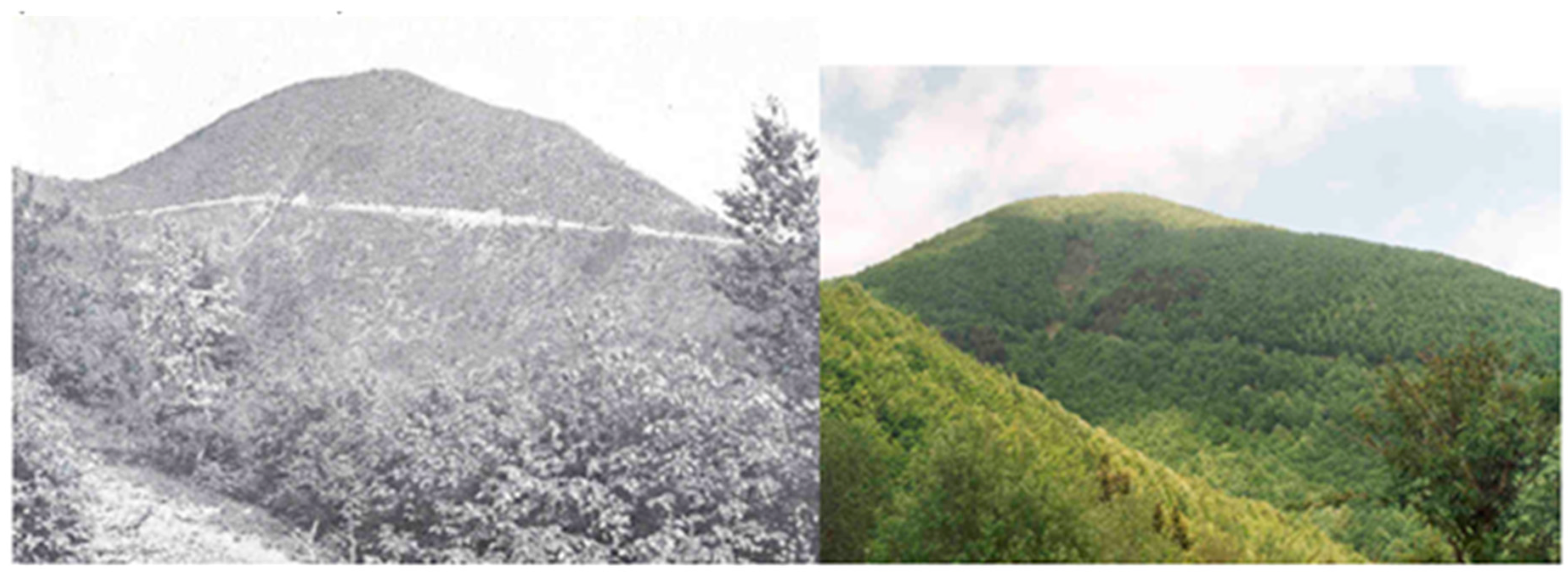
Figure 3.
Photos of Tresca Mountain (1473 m. a.s.l.) near Porretta Terme (RMB): In the past, say 1914 (left), forests were sparse due to exploitation, while currently the area is forested (right).
Figure 3.
Photos of Tresca Mountain (1473 m. a.s.l.) near Porretta Terme (RMB): In the past, say 1914 (left), forests were sparse due to exploitation, while currently the area is forested (right).

Figure 4.
LULC changes in the RMB between 2003 and 1954 (a), and the LULC of the riparian buffer strips (b).
Figure 4.
LULC changes in the RMB between 2003 and 1954 (a), and the LULC of the riparian buffer strips (b).

Figure 5.
Time series of the Reno River mean yearly flow rate and linear trends with 95% confidence limits (green) and the prediction limits (grey) of the least squares fit model.
Figure 5.
Time series of the Reno River mean yearly flow rate and linear trends with 95% confidence limits (green) and the prediction limits (grey) of the least squares fit model.

Figure 6.
Box and whisker plots of monthly flow rates between 1921 and 2013 (a), and of the subpopulations: 1921–1959 and 1960–2013 (b).
Figure 6.
Box and whisker plots of monthly flow rates between 1921 and 2013 (a), and of the subpopulations: 1921–1959 and 1960–2013 (b).

Figure 7.
Seasonal SSY and the linear trend of yearly SSY (a). Seasonal SSY variations of 1942-59 and 1960-78 years respect to seasonal average of 1942 to 1978 years (b).
Figure 7.
Seasonal SSY and the linear trend of yearly SSY (a). Seasonal SSY variations of 1942-59 and 1960-78 years respect to seasonal average of 1942 to 1978 years (b).

Figure 8.
Linear relation between SSY and mean (Qmean) and maximum (Qmax) flow rate.

Figure 9.
Local climate change: Linear trends of maximum and minimum temperature (Tmax and Tmin) for mountain (Mg) and valley (Vg) gauges (a); yearly RMB precipitation with linear trend with 95% confidence limits (green) and the prediction limits (grey) of the least squares fit model (b).
Figure 9.
Local climate change: Linear trends of maximum and minimum temperature (Tmax and Tmin) for mountain (Mg) and valley (Vg) gauges (a); yearly RMB precipitation with linear trend with 95% confidence limits (green) and the prediction limits (grey) of the least squares fit model (b).

Figure 10.
Runoff coefficient observed in the last 90 years (R2 = 0.43) with linear trends, prediction and confidence limits.
Figure 10.
Runoff coefficient observed in the last 90 years (R2 = 0.43) with linear trends, prediction and confidence limits.

Figure 11.
Reno River transect between Casalecchio Chiusa and Porretta Terme, with corresponding locations.
Figure 11.
Reno River transect between Casalecchio Chiusa and Porretta Terme, with corresponding locations.

Figure 12.
Reach R1 near Porretta that is more torrential (left) and R3 near Chiusa Casalecchio with fine sediments (right): Riparian forest shows a strong development.
Figure 12.
Reach R1 near Porretta that is more torrential (left) and R3 near Chiusa Casalecchio with fine sediments (right): Riparian forest shows a strong development.

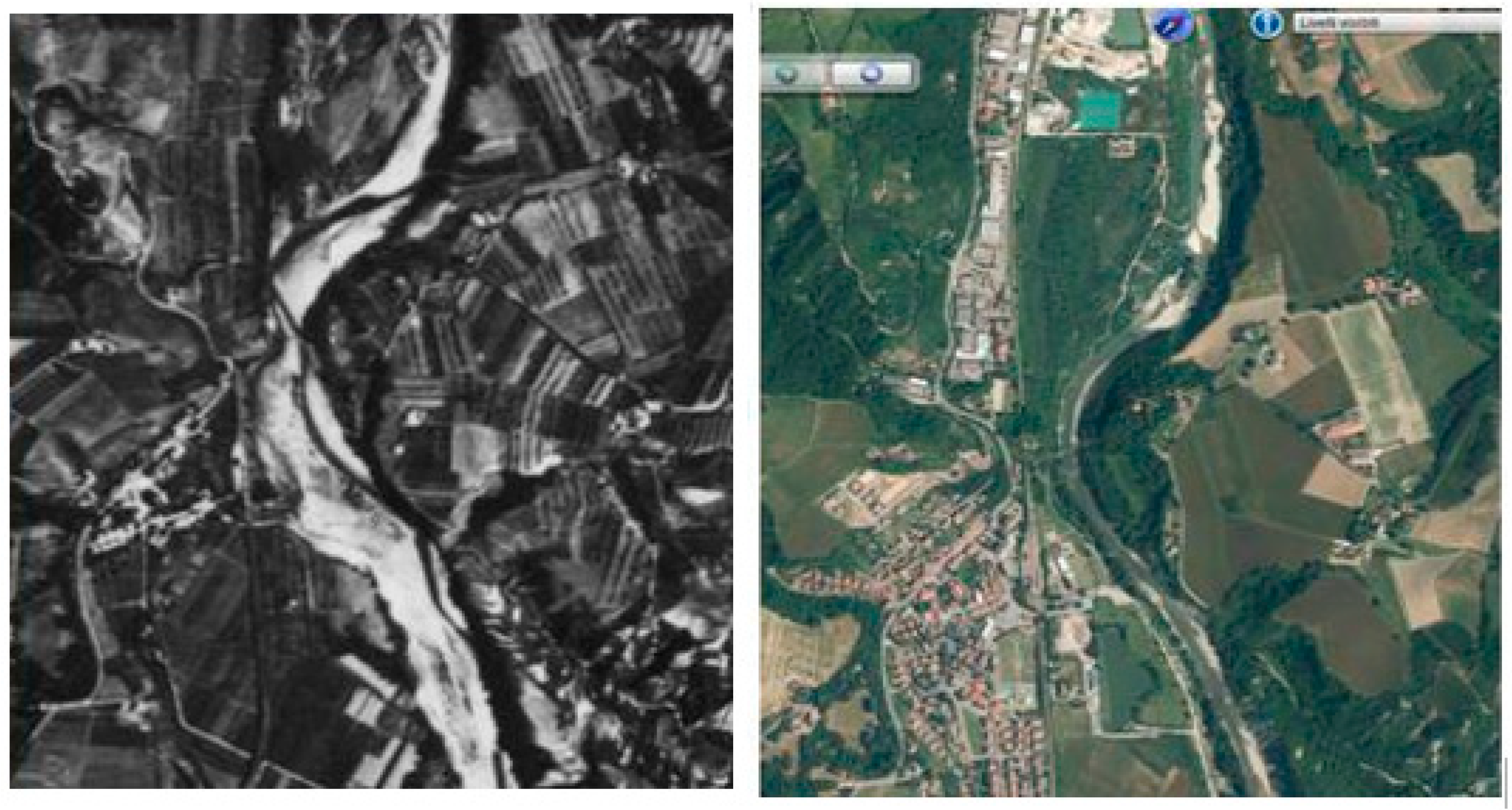
Figure 13.
Reach 2 near Marzabotto village. Wide stream and area covered with crops in 1954 (left), but urban areas and a narrow stream in 2003 (right).
Figure 13.
Reach 2 near Marzabotto village. Wide stream and area covered with crops in 1954 (left), but urban areas and a narrow stream in 2003 (right).


Table 1.
Available data set and its properties.
| Parameter | Data Record | Number of Years Available | Area | Lenght | Data Source |
|---|---|---|---|---|---|
| River flow rate (m3 s−1) | 1921–2013 | 87 | 1061 km2 | 80 km | SIMI, ARPA |
| Suspended sediment yields (Mg km−2) | 1942–1978 | 31 | 1061 km2 | 80 km | SIMI |
| Land Cover RMB | 1954&2003 | 2 | 1061 km2 | na | GAI flight, Quickbird |
| Land Cover Reno riparian buffer strips (R1–R3) | 1954&2003 | 2 | 27.3 km2 | 54.5 km | GAI flight, Quickbird & field survey |
| Reno riverbed morphology (R1–R3) | 1954&2003 | 2 | 27.3 km2 | 54.5 km | GAI flight, Quickbird & field survey |
| RMB Precipitation (mm) | 1921–2013 | 87 | 1061 km2 | na | SIMI, ARPAE |
| Maximum and minimum temperature (°C) * | 1928–2007 1936–2007 | 7670 | na | na | SIMI, ARPAE |
* The two periods correspond to the two meteorological stations—one in the valley and another in the mountains, that were analyzed separately in order to highlight differences between them.
Table 2.
Summary statistics of mean and maximum annual flow rate (Q) and suspended sediment yield (SSY)—average yearly data.
Table 2.
Summary statistics of mean and maximum annual flow rate (Q) and suspended sediment yield (SSY)—average yearly data.
| Parameter | Years Available | Average | Minimum | Maximum |
|---|---|---|---|---|
| Qmean (m3 s−1) | 77 | 23.4 ± 7.0 | 13.3 (in 1938) | 42.4 (1937) |
| Qmax (m3 s−1) | 77 | 68.7 ± 25.96 | 21.8 (in 2007) | 143.1 (in 1959) |
| SSY (Mg km−2) | 31 | 935 ± 440 | 217 (in 1962) | 2250 (in 1951) |
Table 3.
Main features of the Reno reaches.
| Feature | R1 | R2 | R3 | |||
|---|---|---|---|---|---|---|
| 1954 | 2003 | 1954 | 2003 | 1954 | 2003 | |
| Length (km) | 20.9 | 23.0 | 10.6 | |||
| Mean bed slope (%) | 0.53 | 0.45 | 0.31 | |||
| Average valley width (m) | 166 | 423 | 1476 | |||
| Average channel width (m) | 90–100 | 30–40 | 90–300 | 30–70 | 300 | 90 |
| Average channel area (ha) | 210 | 80 | 206 | 78 | 299 | 61 |
© 2019 by the authors. Licensee MDPI, Basel, Switzerland. This article is an open access article distributed under the terms and conditions of the Creative Commons Attribution (CC BY) license (http://creativecommons.org/licenses/by/4.0/).
Share and Cite
MDPI and ACS Style
Pavanelli, D.; Cavazza, C.; Lavrnić, S.; Toscano, A. The Long-Term Effects of Land Use and Climate Changes on the Hydro-Morphology of the Reno River Catchment (Northern Italy). Water 2019, 11, 1831. https://doi.org/10.3390/w11091831
AMA Style
Pavanelli D, Cavazza C, Lavrnić S, Toscano A. The Long-Term Effects of Land Use and Climate Changes on the Hydro-Morphology of the Reno River Catchment (Northern Italy). Water. 2019; 11(9):1831. https://doi.org/10.3390/w11091831
Chicago/Turabian StylePavanelli, Donatella, Claudio Cavazza, Stevo Lavrnić, and Attilio Toscano. 2019. "The Long-Term Effects of Land Use and Climate Changes on the Hydro-Morphology of the Reno River Catchment (Northern Italy)" Water 11, no. 9: 1831. https://doi.org/10.3390/w11091831
Note that from the first issue of 2016, this journal uses article numbers instead of page numbers. See further details here.