Clogging Issues with Aquifer Storage and Recovery of Reclaimed Water in the Brackish Werribee Aquifer, Melbourne, Australia

1
KWR Watercycle Research Institute, 3430 BB Nieuwegein, The Netherlands
2
Faculty of Civil Engineering and Geosciences, Delft University of Technology, 2628 CN Delft, The Netherlands
3
City West Water, Footscray 3011, Australia
*
Author to whom correspondence should be addressed.
Water 2019, 11(9), 1807; https://doi.org/10.3390/w11091807
Submission received: 30 June 2019
/
Revised: 22 August 2019
/
Accepted: 24 August 2019
/
Published: 30 August 2019
(This article belongs to the Special Issue Managed Aquifer Recharge for Water Resilience)
Abstract
:As part of an integrated water-cycle management strategy, City West Water (CWW) is conducting research to develop an aquifer storage recovery (ASR) scheme utilizing recycled water. In this contribution, we address the risk of well clogging based on two ASR bore pilots, each with intensive monitoring. Well clogging is a critical aspect of the strategy due to a projected high injection rate, a high clogging potential of recycled water, and a small diameter injection borehole. Microscopic and geochemical analysis of suspended solids in the injectant and backflushed water, demonstrate a significant contribution of diatoms, algae and colloidal or precipitating Fe(OH)3, Al(OH)3 and MnO2. CWW is, therefore, testing additional prefiltration that includes a 20 μm spin Klin disc and 1–5 μm bag filter operating in series. In this paper, we present optimized methods to (i) detect the contribution of the injectant and aquifer particles to total suspended solids in backflushed water by hydrogeochemical analysis; and (ii) predict and reduce the risk of physical and biological clogging, by combination of the membrane filter index (MFI) method of Buik and Willemsen, a modification of the total suspended solids method of Bichara and an amendment of the exponential bacterial growth method of Huisman and Olsthoorn.
Keywords:
ASR; recycled water; well clogging; geochemical analysis; filtration; biofouling; risk management1. Introduction
The use of reclaimed or recycled water is on the rise worldwide, mainly because of (i) water scarcity due to exponential population growth and climate change, and (ii) the need to reduce the pollution load from waste water that ends in surface water systems [1,2].
As part of an integrated water-cycle management strategy for the fast growing city of Melbourne, City West Water (CWW) is conducting research to apply aquifer storage recovery (ASR) utilizing recycled water [3]. This non-potable water is to be injected and stored during winter in a brackish, anoxic sand aquifer at 220–250 m below ground level (BGL), and recovered during peak demand periods in summer. The purpose is to reduce drinking water consumption by supplying recycled water via a third pipe system. The infiltration water will be Class A recycled water, which is fit for high exposure uses (not for drinking water consumption), diluted with desalinated water (by reverse osmosis). Class A recycled water comes from Melbourne Water Corporation’s Western Treatment Plant, which produces recycled water from a series of anaerobic and aerobic lagoons followed by UV disinfection and chlorine disinfection.
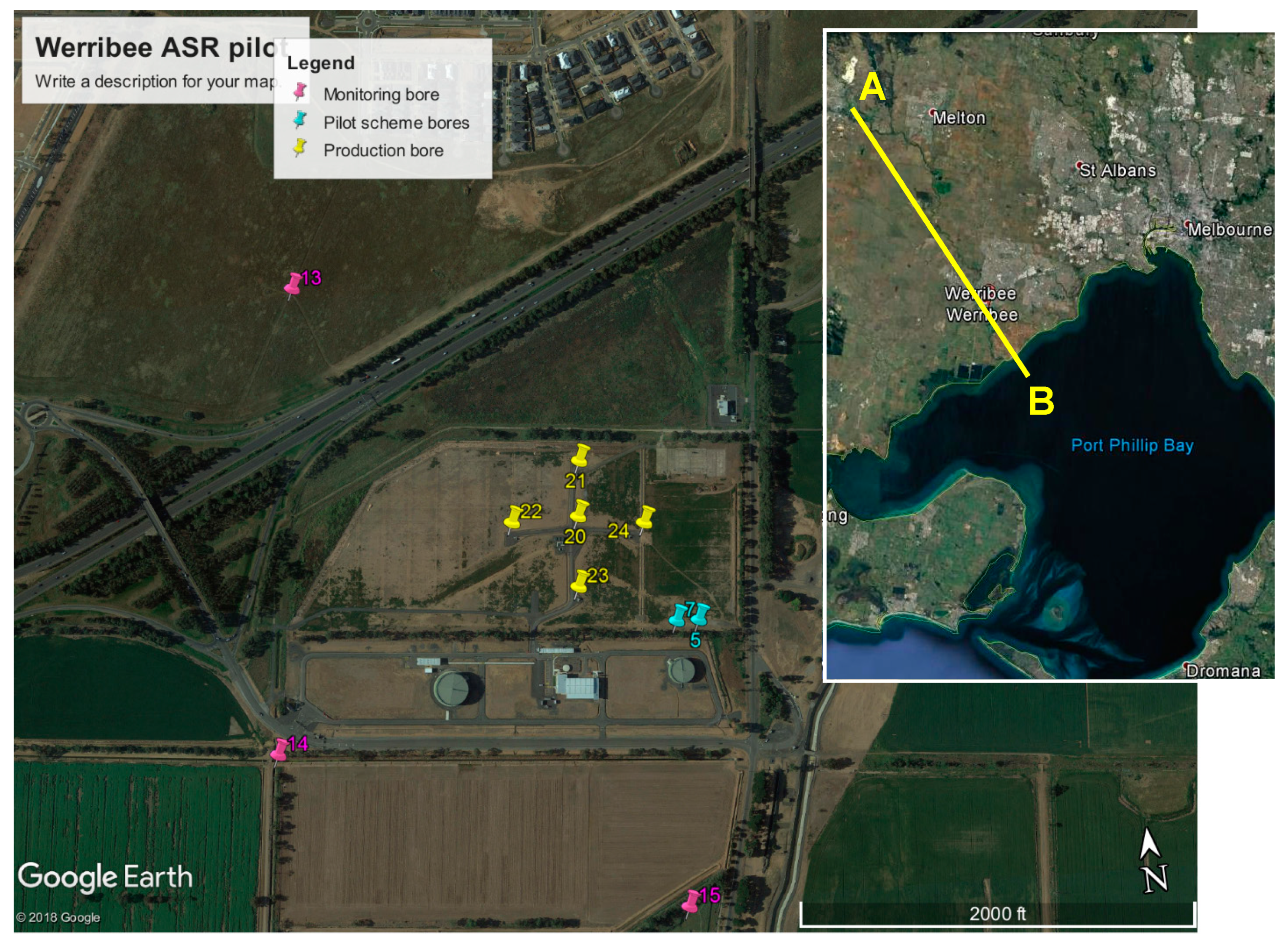
Several studies have confirmed the viability of ASR at the trial site (West Werribee, west of Melbourne; Figure 1), based on the acceptable overall quality of the infiltration water [4,5], the transmissivity and dispersivity of the aquifer and background flow [4], geochemistry of aquifer [6,7], the ambient water quality in the target aquifer [5], predicted water quality of recovered water [6,8], and economic, societal and water security implications [3].
Nevertheless, two recognized main risks still warrant ongoing investigation of respectively the actual well clogging risk [7,9], and risk caused by undesired water quality changes in the target aquifer [5]. Injection well clogging can be extremely cumbersome leading to high costs due to monitoring, maintenance, premature well replacement, intensification of pretreatment or addition of more wells [9,10,11,12].
Common water quality issues with ASR application, especially when dealing with recycled water, consist of (i) mobilization of trace metals and arsenic by pyrite oxidation [13]; (ii) lack of full elimination of high concentrations of NO3 and PO4, (iii) the formation of trihalomethanes and haloacetic acids by chlorination [14]; (iv) the persistence of some pathogens and organic micropollutants in the aquifer [2,15]; and (v) the undesired admixing of ambient groundwater (total dissolved sSolids (TDS), H2S, natural radionuclides) [5]. There are also concerns about potential changes in the microbiota and stygofauna (taxa that spend their whole life cycle in groundwater) by introducing among others oxygen, algae and xenobiotic compounds [16,17,18].
In this contribution, we evaluate the risks of ASR well clogging based on a short ASR pilot investigation in 2012, and an ongoing ASR pilot test which started in 2017. We present hydraulic, geochemical and microscopic data, diagnose the main clogging causes, and indicate how to mitigate or prevent the problem.
2. Materials and Methods
2.1. Aquifer Storage Recovery (ASR) Pilot Tests
Two pilot tests were conducted in 2012 and 2017–2019, respectively. The first used one injection bore (well 5) and well 7 served as a monitoring bore (Figure 1). The second test (still running) consists of one injection bore (well 20), wells 21–24 as nearby and wells 12–15 as remote monitoring bores (Figure 1).
Details of the ASR cycling scheme are summarized for both pilot tests in Table 1. The 5 clustered wells 20–24 are part of the future ASR system, which is expected to infiltrate 0.5–1.0 Mm3/year during winter time and to recover ~80% of this volume during summer time, depending on demand. The ASR wells include a stainless steel (316) telescopic design, with internal diameter of 350 mm in the upper section, 200 mm in the lower section (incl. well screen), and screen aperture ranging from 0.4 to 0.8 mm. They are not supplied with a gravel pack nor a downhole flow control valve.
2.2. Characterization of Target Aquifer
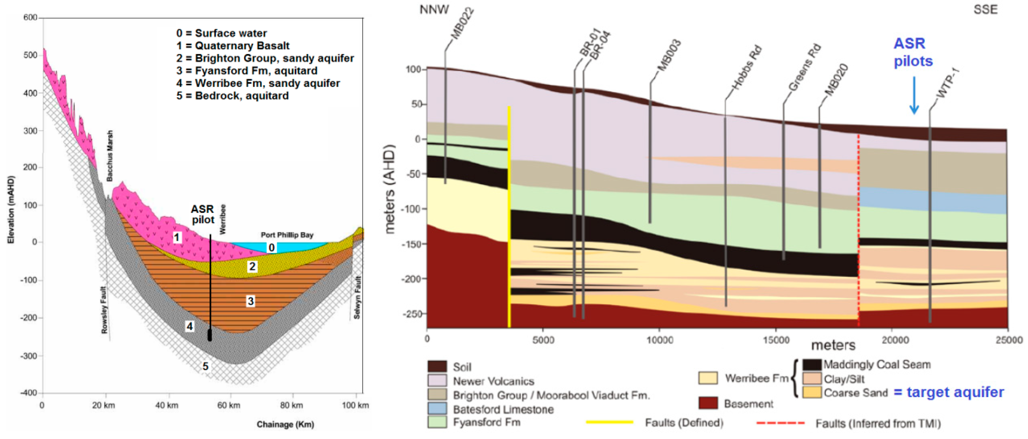
The ASR target aquifer consists of the coarser grained sequences within the Lower Werribee Formation (LWF) of Early Tertiary age. It is formed by a heterogeneous sequence of sands, silts, clays and lignite, slightly dipping on average in SE direction. The LWF rests on nearly impervious Lower Paleozoic basement rock, and is overlain by 200 m of (un)consolidated sediments (Figure 2).
In the LWF, the sands are typically found between 220 and 240 m below sea level. They vary in grain size (0.1–0.8 mm) and thickness (3–22 m) over short distances. Most wells have two screen sections separated by a blind casing interval of 2–4 m in the middle, where the aquifer is too silty. Average aquifer characteristics are listed in Table 2, based on pumping tests [4], breakthrough curves [5], sedimentological and geochemical analysis of aquifer cores [7,19].
2.3. Water Quality Analysis
Samples of infiltration water and of water from wells were taken at the well head, with and without prior filtration over 0.45 μm in the field. The standing volume in well screen and riser was always evacuated 3 times prior to sampling. In the field, pH, electrical conductivity (EC), temperature, oxidation reduction potential (ORP) and O2 were measured at selected intervals. Sensors of EC, temperature and water pressure, installed at screen depth in the wells, have been registered between 3 and 10 min.
Sample container type, preservation method, holding time and analytical method were as recommended by ALS Environmental [22], which performed the analyses on a wide spectrum of parameters: general chemistry (pH, EC, turbidity, total suspended solids (TSS), algae), major ions, nutrients, total and dissolved organic carbon (TOC and DOC, respectively), (trace) metals, gases (O2, CO2, H2S, CH4), disinfection by-products, industrial organic micropollutants, pesticides, pharmaceuticals, radionuclides, and microbiological parameters. Sampling frequency was on average on a weekly basis but fine-tuned to the duration of ASR cycles, the breakthrough in monitoring wells, and costs of analytical packages [8].
2.4. Analysis of Suspended Matter during Backflushing
Backflushing of the ASR well, with a 2–3 times higher pumping than injection rate, directly or after juttering, is a method to unclog the well screen or bore hole wall. Samples of the turbid backflush water were taken from ASR well 20 on 4 occasions (A–D): during injection cycle 2 (A), two well redevelopments after cycle 3A (B, C) and during injection cycle 3B (D), respectively. Samples of unfiltered water were taken after evacuation of 9–12 m3, corresponding with ~1 standing well volume. The samples (3.6–4.2 L) were transported to the lab in an upright position, in the dark and cooled at 4 °C, without shaking. In the lab, these samples were kept in the dark at 4 °C for 2 days in upright position without shaking/tremors, in order to let the suspended matter settle. Subsequently as much clear water as possible was slowly decanted or sucked out, containing on average 95% of all water with on average only 2.7% of all TSS: 1 mg TSS/L in 0.95 × 4 L and 690 mg TSS/L in 0.05*4 L yields indeed 100 × (0.95 × 4 × 1)/(0.95 × 4 × 1 + 0.05 × 4 × 690) = 2.7%, which is neglected in Equation (1). The decanted water was analyzed, after 0.45 μm filtration, for all main constituents (incl. pH and EC), DOC and trace elements. This yields the dissolved fraction.
The remaining fluid (0.2–0.5 L) with 97% of all TSS was first analyzed for TSS, and subsequently, after nearly complete destruction with strong suprapure HNO3 at 95 °C, analyzed for TOC, total concentration of main constituents (excluding Cl, HCO3, NO3) and trace elements.
The analytical results of the dissolved and suspended fraction in mg/L were used to calculate the composition of the suspended material as follows:
where: XSS = content of component X in suspended solids (ppm = mg/kg dry weight); XT = total X concentration in water with suspended solids (mg/L); XH2O = concentration of X dissolved in water (mg/L); TSS = total suspended solids in water (mg/L)
2.5. Clogging Predictor Based on Membrane Filter Index (MFI)
Buik and Willemsen [23] used the membrane filter index (MFI; [10,24,25]), well and hydrogeological parameters to predict the clogging rate of recharge wells, based on the following semi-empirical equation (without dimensional homogeneity):
with:
where: vCLOG = clogging rate (m/a); MFI = 0.45 μm membrane filter index (s/L2); tEQ = total amount of equivalent full load hours per year (h); vDIR = entrance velocity on borehole wall (m/h); D50 = median grain size diameter of aquifer (μm); QIN = mean infiltration rate when well is recharging (m3/h); rB = radius of borehole (m); L = length of well screen (m); Kh = horizontal hydraulic conductivity (m/d).
vCLOG = 2 × 10⁻⁶ × MFI × tEQ × VDIR2/(Kh/150)1.2,
Kh = 150(D50/1000)1.65 or Kh = T/D,
VDIR = QIN/(2πrBL),
2.6. Clogging Predictor Based on Total Suspended Solids (TSS)
Another way to predict the physical clogging rate, is to relate the decrease in flow rate of an injection well (Qt/Q0) to the ratio of the total input of suspended solids after a given injection time, to the open area of the external borehole wall (AOPEN). On the basis of many experimental data Bichara [26] showed an interesting plot of that relation. Notwithstanding the scatter of his many data, an average linear trend can be used to estimate the decline in flow rate of an injection well by particle clogging:
with:
where: Qt, Q0 = injection rate at time t since start and at start (t = 0), respectively (m3/h); ε = aquifer porosity (-); t = time since injection start (day); t10 = injection period needed to reduce flow by 10% (day).
Qt/Q0 = 100 − 17.5TSS × QINt/AOPEN, if >0, else 0
t10 = 10 t/(100 − Qt/Q0), if >0, else 0
AOPEN = 2πrBεL, (m2)
2.7. Predictor of Bioclogging
Bioclogging can be simulated by the following equation (modified after Huisman and Olsthoorn [27], by introducing a lag time), which calculates the buildup of bacteria in infiltration wells:
where: N0 = average number of bacteria in input (n/m3); Nt = average number of bacteria at and behind bore hole wall, at time t (n/m2); t = time since injection start (day); tLAG = lag time during which bacteria do not reproduce (day); TD = doubling time for bacterial population (day); VDIR = entrance velocity on borehole wall, see Equation (4) (m/day).
Thus, it is assumed that each input bacterium is filtered out at the borehole wall and starts multiplying after a specific lag time. The thickness of the biofouled layer (DBAC,t) which fully occupies the aquifer pore space, can be calculated using Equation (9) by assuming that (i) the accumulation of cells with a specific cell volume is taking place on the borehole wall and behind that, both with open space AOPEN, and (ii) there is no open space between bacteria:
where: vCELL = spherical volume of each cell (m3); ε = aquifer or gravel pack porosity (-).
A more realistic model sets a limit to bacterial growth, based on e.g., the observed change in DOC or biodegradable DOC (BDOC; [28]). The available data show a very small decline of the injectant during short storage or recovery cycles (1–2 days) for DOC (<0.5 mg C/L) and BDOC (~0.2 mg C/L). This observed consumption of BDOC during a 1–2 days lasting storage or recovery cycle (ΔBDOC; mg C/L), is the sum of bacterial respiration (BaR) and biomass production (BoP; [29]), so that:
where: QIN = injection rate (m3/d); fBoP = BoP/(Bop + BaR) = fraction of ΔBDOC consumed by bacterial respiration (-);ΔBDOC = consumption of biodegradable DOC (mg C/L).
We assume that ΔBDOC represents steady state, and that it approaches consumption by the total number of active cells at maximum growth, so that:
NtMAX can also be calculated with Equation (8) by replacing t by tMAX, which is defined as the time since start of exponential bacterial growth to the maximum level of growth. Combination of this Equation (8) with Equations (11) and (4) yields after rewriting, for both limitation cases:
3. Results
3.1. Injection Well Clogging
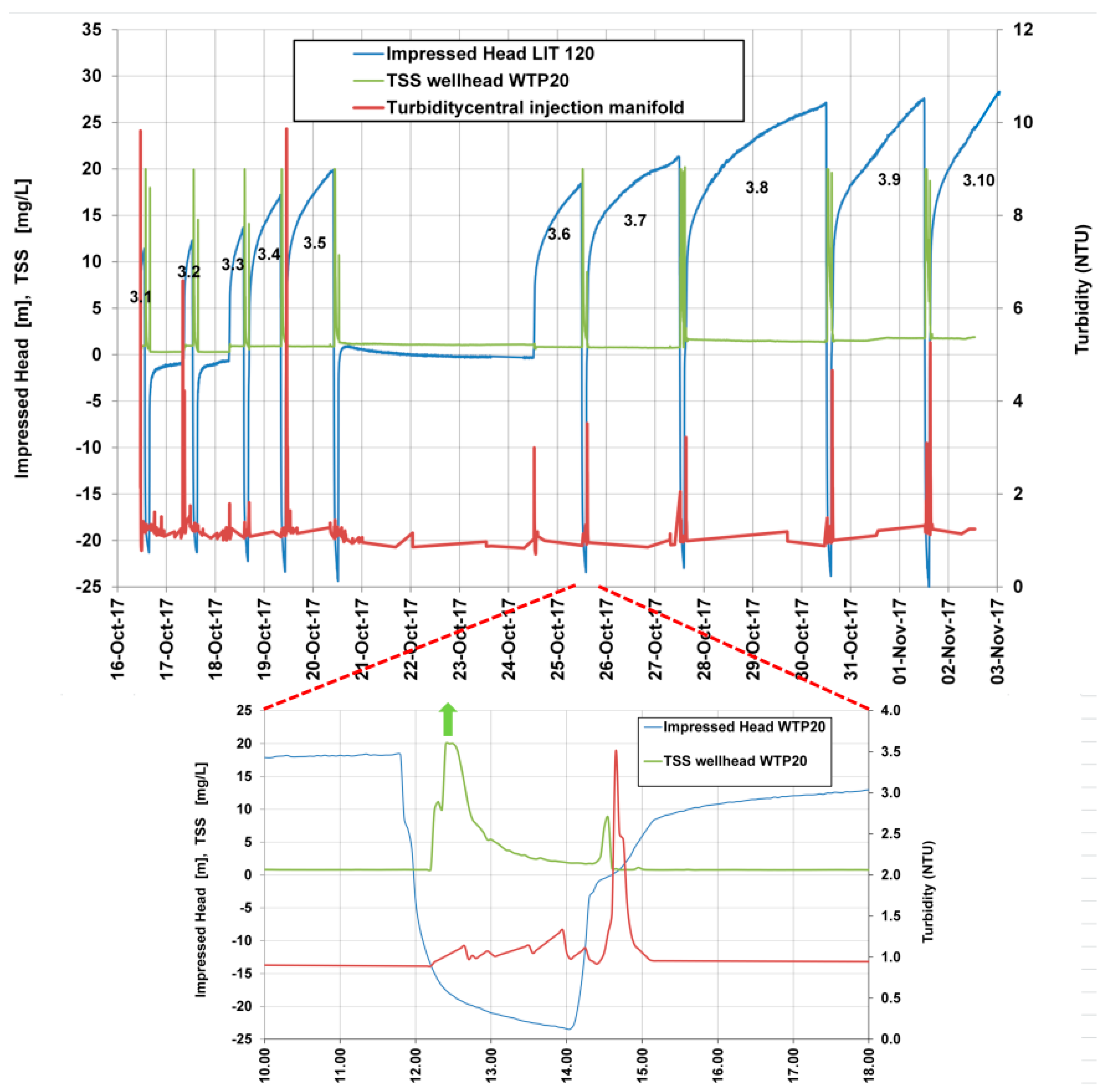
A typical pattern of impressed head and drawdown, TSS (at well head) and turbidity (in central injection manifold) for ASR well 20 during ASR Cycle 3, is shown in Figure 3. The peaks of TSS and turbidity coincide with 9 short flow reversals due to backpumping (108 m3/h) and reinjection (54 m3/h). This triggered the mobilization of fines from the borehole wall and probably also from the well itself. TSS peaked during both switches (injection to backpumping, and vice versa), whereas turbidity only peaked during the switch from backpumping to injection, due to the position of the turbidity sensor right after the injection pump. The TSS sensor’s output is maximum 20 mg/L in order to focus on lower level variability, but short peaks of up to 43.5 (=870/20) mg/L have been measured (Table 3).
The backflushing is successful in removing the bulk of clogging material, but a growing residual (chronic) clogging is remaining, as evidenced by the rising impressed head (Figure 3) during identical successive injection runs such as 3.7, 3.9 and 3.10 (not fully shown). The clogging process was linear during the 15 days lasting injection period 3 of the first ASR trial [4], which is typical for clogging mainly caused by particles [10].
3.2. Results of Hydrogeochemical Analysis of Suspended Material
The composition of the suspended solids was calculated for each sample taken during the 4 backflushing events A–D, by applying Equation (1). Each sample was taken after on average 1.5 days injection of 1950 m3, and after ~5 min backflushing (corresponding with 11 m3 and 1 standing volume in the well). The results are presented in Table 3, together with a summary of the geochemical analyses of aquifer cores and TSS of the injectant. Zero values mean that XT equals XH2O, so that practically all of X is in dissolved form. Empty cells in Table 3 (with ‘-’) mean no data available.
3.2.1. Average Composition
In Table 3, the average composition is listed for samples of events A–C. The sample of event D was excluded because it refers to a different input (see Section 3.2.2). On average ~8.4% of the suspended material has thus been identified and quantified. This means that 92% is not covered by the analysis, due to (i) lack of dissolution in the acid and oxidizing leach (notably quartz), (ii) lack of the usual conversion of the elements in their oxide form, and (iii) no inclusion of H2O which is present in the crystal lattice of some minerals such as amorphous Fe(OH)3 and Al(OH)3.
The highest contents are noticed for the following main constituents, in decreasing order: Si (underestimated due to incomplete extraction), Fe, Al, S, C, Mn and P. The true Si content is estimated at max 37% (not the 1.6% extracted; 37% = (100% – sum XnO-bound H2O)/MWSiO2, where XnO = all individual elements, SiO2 excluded, each transformed in its oxide form, e.g., C in CH2O and Fe in Fe2O3). Si is mainly linked to SiO2 as quartz and diatoms. Concentrations of Na, K, Ca and Mg were <0.2%.
The high S content very likely indicates the presence of iron sulfide particles, because gypsum can be excluded and the alternative, organic matter, contains on average only 1.8% S (0.018 × CORG = 127 ppm S). Thus assuming the remaining 10,045 ppm (=10,172 – 127) to be FeS2 (pyrite) requires the presence of enough Fe, namely 8858 ppm. This would mean that the TSS contains an excess of 13,420 ppm Fe, which could be Fe(OH)3 or Fe2O3 deriving from the source water directly or indirectly (from biofilms on the transmission pipeline, a storage tank or ASR well casing), and from rust particles from corroding stainless steel parts of the transmission pipeline, storage tank or ASR well casing).
3.2.2. Trends
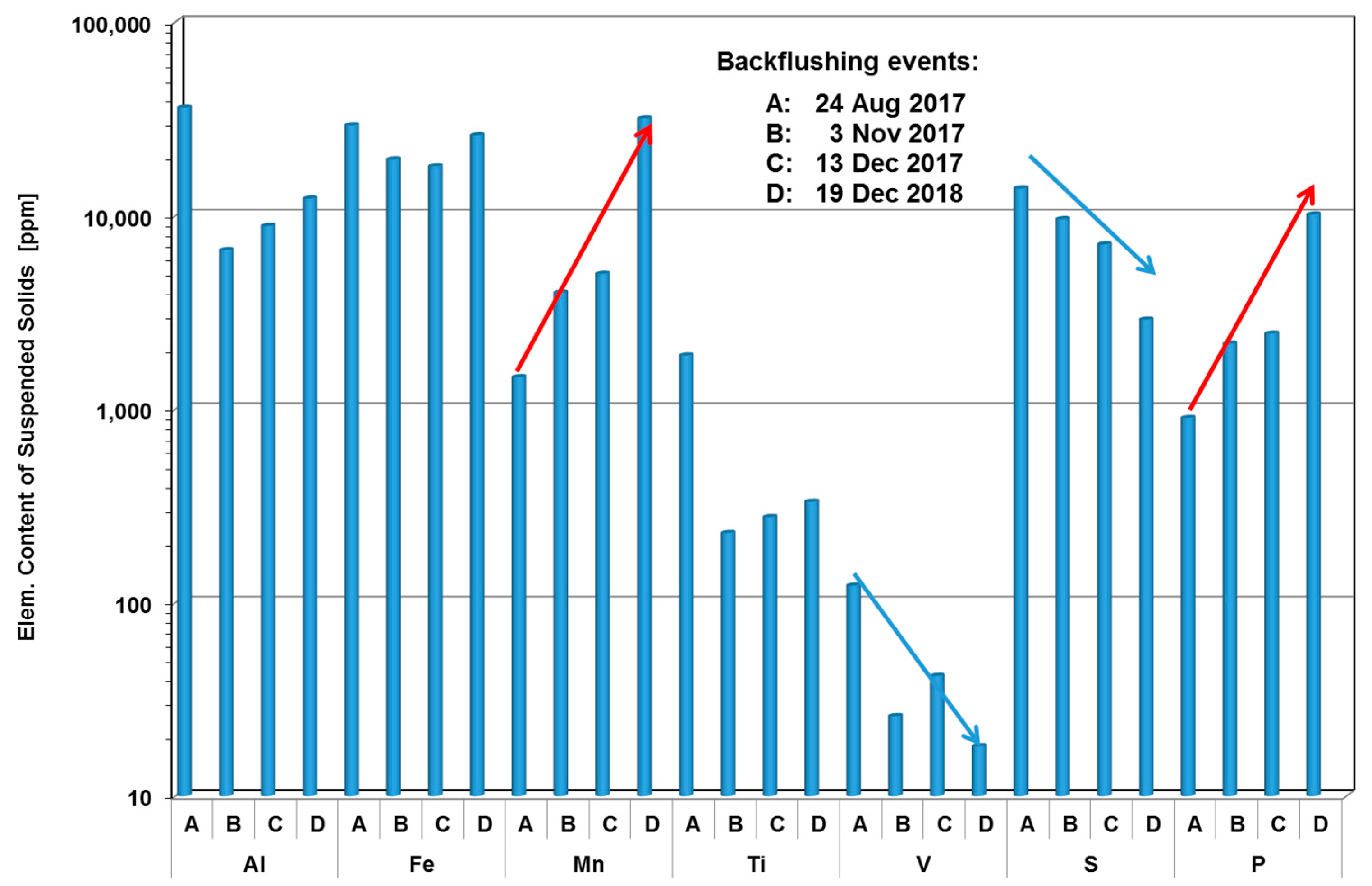
The composition of samples from backflushing events A–D varies over time, in a more or less systematic way for the following elements (red numbers in Table 3; Figure 4): (i) P and Mn steadily increasing, and (ii) S, FeS2, Fe-FeS2, Fe/Mn and V steadily decreasing. This indicates that over time, the infiltration water input is contributing more (P and Mn) and aquifer material less (pyrite and V) to TSS in the backflushed water. This agrees with expectations.
The sample from backflushing event D showed a remarkable overall concentration increase (S and V excluded). The reason for this increase is not clear, but could be related to the applied prefiltration step, which resulted in the accumulation of finer grained particles on the borehole wall and behind. These finer grained particles could contain less quartz particles and more soluble material.
3.2.3. Comparison with Aquifer Cores and Infiltration Water
In Table 3, the element content of TSS can be compared with the aquifer core data and with the average TSS composition of infiltration water. We selected the mean TSS composition of backflush events A–C, the injectant (without prefiltration) and the core data from monitoring well 3 (~1 km south of well 15, Figure 1). The core had about the same extraction and geochemical analysis as TSS, and showed a similar aquifer sedimentology as well 20. These data have been used in Table 3 to estimate the fraction of suspended particles in the infiltration water (α) and of aquifer particles (1 – α) contributing to the mean TSS composition of the backflush sample. The following unmixing equation for 2 end-members was used:
Fraction α appears lowest (0.15) for S (and associated FeS2 and Fe-FeS2), so that practically all S (pyrite bound) in TSS is derived from the aquifer, as deduced earlier. Fraction α increases slightly for Cu, Mn, Co, V and Fe (from 0.21 to 0.40, respectively), which indicates that the aquifer is forming their mean supply during events A–C. Only P, Cr, Ni and Sr seem to be largely delivered by the injectant during events A–C, Cr perhaps even totally. The calculated α numbers are not very accurate due to temporal variations in the injectant and spatial variations in aquifer geochemistry.
An important assumption in this interpretation is, that the mentioned ions did not (co)precipitate in the water sample during transport from well to the lab and during 2 days of air-tight bottle detention prior to the separation of decantable fluid from the remaining high TSS liquid. We checked this by comparing the infiltration water with the decanted fluid, and the decanted fluid of the first with the last sample. Concentrations of dissolved Al, Fe, Mn NO3, NH4 and PO4 did not show significant changes, indicating that the potential contribution of Fe or Mn flocs formed by oxidation of the backflushed water was rightly ignored.
3.3. Results of Microscopic and Particle Size Analysis of Suspended Material
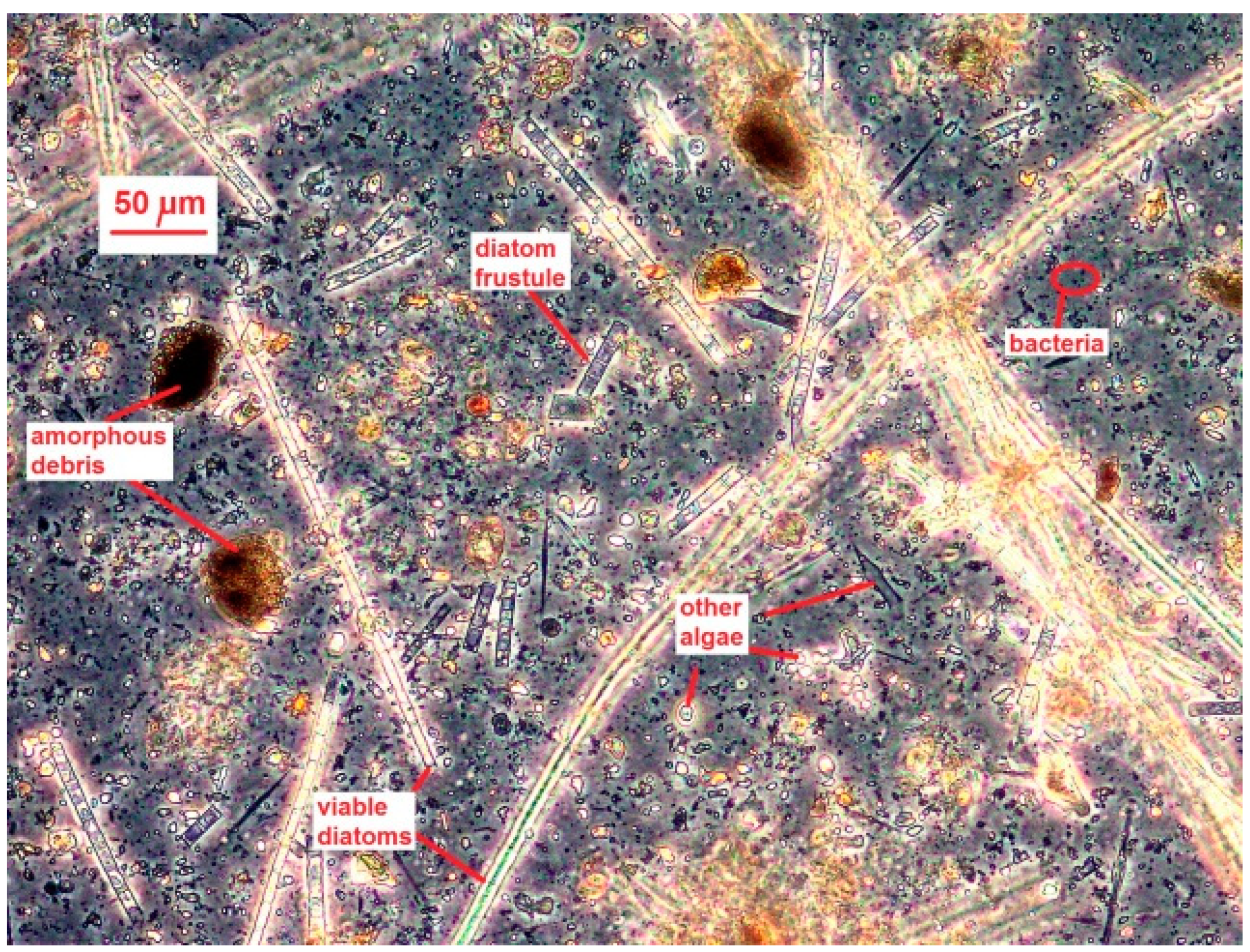
Suspended material in source water and in backflushed water was examined by microscopic analysis. The results are summarized in Table 4, and a characteristic image is shown in Figure 5. The diatoms and other algae in the backflushed water are clearly derived from the infiltration water input, because they are too undamaged and some are even still viable.
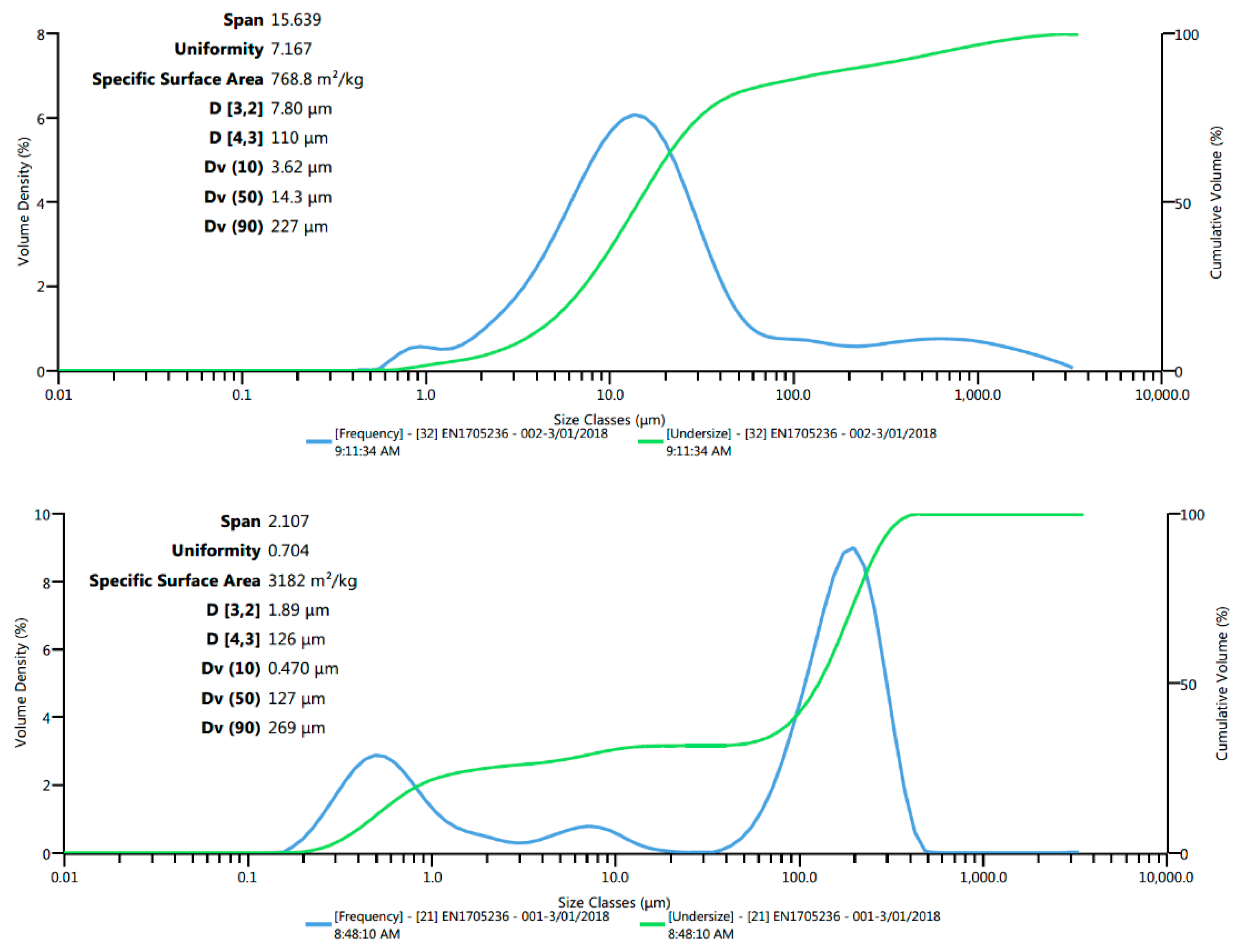
Results of particle size analysis by Light-Scattering using a Mastersizer 3000 instrument, after sonication or addition of a dispersant, are shown in Figure 6. In the backflushed water, 3 peaks can be observed in the particle size distribution: around 0.5, 7 and 200 μm. In the infiltration water, there is a large peak around 13 μm with 2 small, ill-defined peaks around 0.8 and 800 μm. The difference between both particle size distributions could be not representative due to fluctuations in particle load and particle size distribution of either the infiltration water or backflush water. The peak around 200 μm in the backflush water could be due to either a rather high number of elongate diatoms >200 μm long (Figure 5), which the analyser underestimates due to their shape, or sand intake by the well.
3.4. Evaluation of Clogging Risks
3.4.1. Global Evaluation
ASR well clogging can be caused by any of the following, potential clogging processes (or their concerted action): (i) suspended solids in the infiltration water such as clay, algae, diatoms and Fe(OH)3 flocs, (ii) biofouling due to high concentrations of biodegradable organic matter (TOC, assimilable DOC (AOC), BDOC) and nutrients (PO4, NO3), (iii) air entrainment (gas bubbles formed during cascading in the well), (iv) chemical clogging by precipitates of e.g., Fe(OH)3, MnO2 or CaCO3, (v) clay swelling and clay mobilization due to replacing brackish ambient groundwater with high SAR (sodium adsorption ratio) by fresher, lower SAR injectant, and (vi) permeability reduction by aquifer jamming or aquifer corrosion.
The last four processes are considered of minor importance. Well clogging by gas bubbles is unlikely because of a proper well design [4] and a non-corresponding clogging pattern [10]. The precipitation of minerals by mixing with ambient groundwater during injection phase can be ruled out, because the Fe concentrations in the ambient groundwater are low (0.16 mg/L) and the flow velocity near the well is sufficiently high and reactions are so slow, that reaction products such as iron hydroxide flocks will move relatively far away from the well before being deposited, while the mixing of (sub)oxic water with anoxic ambient groundwater will mainly take place far away from the well. Experiences with and calculations on intentional subterranean iron removal (SIR) [31] indicate that the accumulation of reaction products during both injection and recovery can be neglected on the time scale of one century. SIR is also an unintentional process during ASR [32], which prevents Fe(II) during recovery to reach the ASR well and mix there with any O2 (if this survived the aquifer detention at some depth). The risk of CaCO3 precipitation is also very low, because the injectant and ambient groundwater are undersaturated with respect to CaCO3. Another potential cause of mineral precipitation is chemical instability of the injectant, which can lead to retarded, in-well flocculation of Fe(OH)3 or MnO2. This process is hard to distinguish from the advective transport of suspended particles, and therefore not considered further.
Barry et al. [7] investigated the clogging risk by dispersion of the clay minerals within columns filled with aquifer material, especially within the context of potential future changes in the mixing ratio of Class A water and RO desalinated water. They used a method based on the principles of the ‘Emerson Crumb test’ [33,34,35]. That approach characterizes dispersion using combinations of aquifer materials and source waters by measuring the turbidity increase of the supernatant, relative to that of the water alone, after a period of 48 h. Dispersion of clays in the batch tests was so low that no visible cloudiness was observed in any of the waters tested. Although kaolinite, the predominant clay mineral in the target aquifer, is a non-swelling clay and present within the aquifer storage zone at very low concentrations (<1%), its interaction with low salinity water can still contribute to a reduction in aquifer permeability by detachment from solid surfaces and migration through porous media where it can clog pore spaces [36]. In conclusion, the risk of clay mobilization is (very) low but cannot be ruled out completely, especially not if more RO water is contributing to its mixture with Class A recycled water.
The risk of aquifer permeability losses through aquifer jamming by repeatedly shifting from injection to backflushing, which creates shock waves, is considered low [10]. Aquifer dissolution (not only by the injectant but also by acids applied for well redevelopment) is potentially a risk factor in marley limestone or calcite cemented sandstone aquifers, because the carbonate dissolution will be accompanied by the mobilization of fines that may end up in the pore throats [37,38]. The target aquifer at Werribee is, however, not containing carbonates and thus not vulnerable to this dissolution.
In Table 5, an overview is given of potentially relevant clogging parameters and their levels in the infiltrated Class A recycled water with (second ASR pilot) and without RO water (first pilot), and with (first pilot and cycle 3B of second pilot) and without an onsite prefiltration step (cycles 1–3A of second pilot). The following conclusions are drawn, when comparing the injectant with the given guideline values:
TSS is relatively low (on average 1–2 mg/L), but still above the guideline value for a sandy aquifer (0.1 mg/L). This should lead to physical clogging. Particles containing Fe, Mn and Al probably play a significant role, as deduced from analyzing suspended solids during backflushing, even though the difference between total and dissolved concentrations (the particulate fraction), seems small. MFI is too high, suggesting a high risk of physical clogging. Concentrations of DOC, BDOC ([28]) and AOC ([39]) are high, far above their guideline values. This will lead to biofouling (biological clogging) if without regular backflushing, also because nutrients N + P are not limiting.
3.4.2. Risk of Clogging by Suspended Particles
We quantified this risk by calculating the clogging rate using the modified Bichara method and the Buik and Willemsen method (Section 2.6). The results of calculation are shown for several scenarios in Table 6 (Bichara’s method) and Table 7 (Buik and Willemsen method).
With the modified Bichara method we calculate for ASR well 20 during cycle 3A, resetting the clock after each backflushing event, a flow reduction of about 9% for each day of continuous injection (Table 6). Maintaining the injection rate means that more pressure is needed, which leads to an increase of the impressed head in the well. Intuitively, this increase is proportional to the predicted flow reduction while ignoring temperature effects on viscosity, so that:
where: φ0, φt = the impressed head in the injection well without (significant) clogging, and with clogging at time t since start, respectively (m); f = empirical fit factor, being zero at t = 0, and otherwise >0.
0.01 Qt/Q0 = f φ0/φt so that φt = 100 f φ0/(Qt/Q0)
Application of Equation (16) to the 3-day-long injection period from 27 October up to and including 30 October 2017 (Figure 3), yields an excellent overlap of calculated with measured φt (Table 6), with parameter settings of f = 2 (if t > 0) and φ0 = 10 m. Table 6 also shows how much effect can be expected from reducing the injection rate, TSS input or augmenting the backflush frequency or borehole radius.
For ASR well 20 during cycle 3A, with an MFI value of 47 s/L2, we calculate with the method of Buik and Willemsen [23] a clogging rate of 520 m/a or 1.42 m/day, assuming 100 days of injection a year (Table 7). This high clogging rate looks much smaller than the one obtained with Bichara’s method (4.3 m versus 27 m in 3 days), but vCLOG does not include the water level rise due to unsteady flow as does φt. Table 7 also shows how much effect can be expected from reducing the injection rate, MFI (by enhanced pretreatment) and equivalent full loading hours, or increasing the bore hole radius or implementing all measures to reduce the clogging rate.
3.4.3. Risk of Bioclogging
The results of calculating the number of bacteria (N) and the thickness of the biofouled layer (DBAC) are presented for several scenarios in Table 8, and the bacterial growth curve is presented for selected cases in Figure 7. An unrealistic high DBACT is predicted for scenarios A and E–G of the second Werribee trial, when an unlimited supply of assimilable carbon (and nutrients and O2) is assumed, during a long uninterrupted injection run. The observed consumption level of BDOC in the aquifer (ΔBDOC) is believed to represent the biodegradable fraction of DOC, which is then used for both respiration and biomass production. The concentration of ΔBDOC (~0.2 mg C/L) is much lower than the NO3 and PO4 concentrations in the injectant (Table 5) and is, therefore, considered the growth-limiting factor.
When we include growth limitation, then much less bacteria are accumulating in a much thinner biofouled layer: e.g., in case of Werribee scenario A, the calculated total number of bacteria decreases from 6.1 × 10¹⁶ to 1.0 × 10¹⁴ m−2 and the thickness of the biofouled layer declines from 173 to 0.29 mm, in case of BDOC limitation (Table 8).
These predictions are hampered by many imperfections due to among others: (i) inaccuracy of parameters, especially ΔBDOC; (ii) accumulation of dead bacteria by lack of e.g., oxygen, (iii) accumulation of suspended particles other than bacteria, (iv) incomplete removal of biofouling and accumulated fines during backflushing, and (v) erosion by flowing water and predation by higher organisms.
The presented model calculations thus only serve the purpose of doing a sensitivity or risk analysis. What can we do to lower the risk of biological well clogging? The various scenarios in Table 8 reveal that this risk can be lowered by (i) further pretreatment to reduce N0 (requires chlorination, advanced oxidation or reverse osmosis) and BDOC (requires granular activated carbon filtration or slow sand filtration), (ii) chlorination to reduce N0 and extend tLAG (this may raise BDOC and the capacity to oxidize aquifer minerals however), (iii) augmenting the frequency of backflushing (which reduces t), (iv) making wells with a larger AOPEN, especially by drilling larger diameter holes, and (v) reducing the injection rate by augmenting the number of wells.
4. Discussion
Clogging is the enemy of managed aquifer recharge (MAR) operations [41,42], and this holds ‘in extremis’ for injection wells, especially in case of siliclastic aquifers. In Werribee, the results obtained during the first and the second ASR trial (up to and including cycles 1–3A), the first with and the second without additional filtration, confirm that well clogging is indeed cumbersome, requiring frequent backflushing (once per 1–3 days), incidental mechanical well regeneration and intensive monitoring of hydraulic heads. The ongoing research with the additional filtration steps in place (Figure 8) shows optimistic preliminary results, to be confirmed when injection phase 3B continues and more data become available.
In this study, we focused on the 2 main causes of well clogging, i.e., physical clogging by suspended solids in the injectant, and biofouling, after evaluating the risks of 4 other causes of well plugging and the results of column studies by [7] with core material from well 20.
Hydraulic head trends indicate a more or less linear increase of clogging, which pleads for physical clogging as the main process [10]. However, injection runs were relatively short, which prevents biofouling to clearly manifest itself with the typical exponential progress and a typical H2S smell during backflushing after a long storage period during which biomass will putrefy. Backflushing could be optimized by raising the pumping rate not 2 but 3 times the normal recovery pumping rate, by occasional backflushing several times, and by limiting the backflushing time to the period with a significant turbidity rise so as to reduce the waste water volume (Pyne, written communication). Chlorination has been applied during both pilots, but could also be optimized (see [42]) to reduce biofouling while keeping the formation of disinfection byproducts low.
We developed a simple method to deduce the composition and origin of the suspended solids removed during backflushing, based on readily available methods. A more direct method is desirable, however, and could consist of (i) TSS collection in the injectant from both filtration units (right panel in Figure 8), (ii) on-site filtration of a high volume sample during backflushing, and (iii) analysis of the material retained on the filters. For the injectant a lower minimum detection limit of TSS is needed (to be lowered from <1 to <0.1 mg/L), for the backflush water the additional analysis of loss on ignition of TSS is desired to estimate its organic matter content.
Microscopic analyses proved very useful to demonstrate the ubiquitous presence of diatoms, other algae, fine amorphous debris and bacteria in TSS of both the infiltration water and the backflushed water. Seasonal algae blooms should, therefore, be translated into an injection stop, possibly aided by on line turbidity measurements coupled to intelligent decision support and specific action protocols [43]. Another option is to utilize tangential columns [44] as an early warning system to prevent injection of e.g., an incidental TSS peak.
With the focus on well clogging by suspended particles and biofouling, we calculated these risks by three well clogging predictors: (i) the method of Buik and Willemsen [23] based on the MFI, well and hydrogeological parameters, (ii) a modification of Bichara’s method [26] based on the ratio of the TSS input after a given infiltration time, to the open area of the external borehole wall, and (iii) a modification of the method of Huisman and Olsthoorn [27] which relates biofouling to the exponential growth of bacteria. Application of the first and second method is straightforward. The third is, however, handicapped by scarcity of relevant data on changes in biodegradable organic carbon (e.g., ΔBDOC) during aquifer detention, and difficult to assess processes such as the lag time (period for bacteria to acclimatize) and growth limitation by either biodegradable carbon, nutrients or oxygen.
5. Conclusions
From the 6 main causes of injection well clogging, suspended particles and biofouling are the most common of ASR bore clogging [10,42]. This also holds for the ASR system in Werribee, as demonstrated by: (i) hydraulic data, geochemical and microscopic analysis of total suspended solids in the injectant and backflushed water, and (ii) 3 well clogging predictors, 2 of which were optimized for this study and are fit for general application. Clogging predictors yield an order of magnitude estimate of the clogging rate, but above all they serve the purpose of doing a sensitivity or risk analysis.
Based on these predictors the following recommendations can be given to reduce the risk of well clogging by suspended particles and biofouling: (i) reduce the TSS input by prefiltration (preferably by applying rapid followed by slow sand filtration), (ii) reduce the injection rate (may require additional wells), (iii) augment the backflush frequency and its performance, (iv) chlorinate or optimize the chlorination to reduce N0 and extend tLAG (this may raise BDOC, however; CWW already applies chlorination and occasionally a shock chlorination), (v) reduce BDOC (requires granular activated carbon filtration or slow sand filtration), and (vi) drill larger diameter holes. The strength of the predictors is that they yield insight into the relative effect of measures taken.
The order of recommendations presented above (i–vi) reflects the order of decreasing priority for the Werribee pilot. In case of a new pilot anywhere, we recommend the following general order of descending priority, with numbering as above: vi > ii > i > iii > iv > v. This order is subject to modifications depending on among others the outcome of the three presented clogging predictors.
Author Contributions
J.O. designed and supervised the pilot trials; P.S. assisted with the monitoring set-up, analyzed the data and wrote the paper with assistance by J.O.
Funding
This research was funded by the Australian Government Department of Environment and Energy in relation to The National Urban Water and Desalination Plan: West Werribee Dual Supply (Aquifer Storage and Recovery) Project and City West Water.
Acknowledgments
City West Water (CWW) gratefully acknowledges the support of the Australian Government in funding the West Werribee ASR Project. KWR thanks CWW for the assignment to assist in their ASR pilot studies, and for publication of results. Matthew Hudson (formerly CWW, now Southern Rural Water, Werribee) contributed to the project at an earlier stage. Two anonymous reviewers, David Pyne and Peter Dillon gave excellent suggestions to improve the manuscript.
Conflicts of Interest
The authors declare no conflict of interest.
Abbreviations
The following abbreviations are used in this manuscript:
| AOC | assimilable organic carbon |
| ASR | aquifer storage and recovery |
| BDOC | biodegradable dissolved organic carbon |
| BGL | below ground level |
| BOD5 | biological oxygen demand in 5 days at 20 °C |
| CWW | City West Water |
| D | aquifer thickness |
| D50 | median grain size diameter of aquifer |
| DOC | dissolved organic carbon |
| EC | electrical conductivity |
| L | length of well screen |
| LWF | Lower Werribee Formation |
| MAR | managed aquifer recharge |
| MFI | 0.45 μm Membrane Filter Index |
| Mm3 | mega cubic meter |
| Nt, N0 | number of bacteria at time t = t and t = 0 |
| ORP | oxidation reduction potential |
| QIN | mean infiltration rate when well is recharging |
| rB | radius of borehole |
| Q0, Qt | injection rate at time t since start and at start (t = 0), respectively |
| RE | recovery efficiency |
| S | aquifer storativity |
| SAR | sodium adsorption ratio |
| t | time since start (day) |
| t10 | injection period needed to reduce flow with 10% (day) |
| T | aquifer transmissivity |
| TD | doubling time for bacterial population (day) |
| TDS | total dissolved solids |
| TEQ | total amount of equivalent full load hours per year |
| tLAG | lag time during which bacteria do not reproduce, e.g., due to chlorination (day) |
| tMAX | time since start of exponential bacterial growth to maximum growth level (day) |
| TOC | total organic carbon |
| TSS | total suspended solids |
| vCLOG | clogging rate |
| vDIR | entrance velocity on borehole wall |
| αL | longitudinal dispersivity |
| ε | porosity |
| ΔBDOC | consumption of biodegradable DOC |
| φ0, φt | impressed head in injection well without clogging, and with clogging at time t = t |
References
- Bixio, D.; Thoeye, C.; De Koning, J.; Joksimovic, D.; Savic, D.; Wintgens, T.; Melin, T. Water reuse in Europe. Desalination 2006, 187, 89–101. [Google Scholar] [CrossRef]
- Kazner, C.H.; Wintgens, T.H.; Dillon, P. (Eds.) Water Reclamation Technologies for Safe Managed Aquifer Recharge; IWA Publishing: London, UK, 2012; p. 429. [Google Scholar]
- Hudson, M.; Muthukaruppan, M. Meeting Melbourne’s future demand of water using aquifer storage and recovery. In Proceedings of the 9th International Symposium on Managed Aquifer Recharge (ISMAR9), Mexico City, Mexico, 20–24 June 2016. [Google Scholar]
- SKM. West Werribee Dual Supply Project–Phase 2 ASR; Unpublished Investigation Report for City West Water; City West Water: Footscray, Australia, 2013. [Google Scholar]
- Stuyfzand, P.J.; Hudson, M. Hydrogeochemical Evaluation of the Werribee ASR Pilot and Operational Trial; Technical Report No. KWR-2016.107; KWR: Nieuwegein, The Netherlands, 2016; p. 91. [Google Scholar]
- Crisalis International. West Werribee Dual Supply Project: Assessment of Geochemical Data. From a Trial of Aquifer Storage and Recovery Using Class A reclaimed Water Injected and Recovered from the Werribee Formation, Technical Report for SKM Pty Ltd. 2012; 56.
- Barry, K.E.; Vanderzalm, J.L.; Page, D.W.; Gonzalez, D.; Dillon, P.J. Evaluating Treatments for Management of ASR Well Clogging: Laboratory Column Study; CSIRO Land and Water, Client Report to City West Water; City West Water: Footscray, Australia, 2015; p. 71. [Google Scholar]
- Stuyfzand, P.J. Water Quality Aspects and Clogging of the Werribee ASR Operational Trial; Technical Report No. KWR 2018.071; KWR: Nieuwegein, The Netherlands, 2018; p. 90. [Google Scholar]
- Dillon, P.; Vanderzalm, J.; Page, D.; Barry, K.; Gonzalez, D.; Muthukaruppan, M.; Hudson, M. Analysis of ASR clogging investigations at three Australian ASR sites in a bayesian context. Water 2016, 8, 442. [Google Scholar] [CrossRef]
- Olsthoorn, T.N. The Clogging of Recharge Wells Main Subjects; Kiwa: Rijswijk, The Netherlands, 1982; Volume 72, p. 136. [Google Scholar]
- Martin, R. (Ed.) Clogging Issues Associated with Managed Aquifer Recharge Methods. IAH Commission on Managing Aquifer Recharge, Australia. 2013. Available online: http://recharge.iah.org/recharge/documents/clogging-MAR-all.pdf. (accessed on 15 May 2019).
- Houben, G.; Treskatis, C. Water Well Rehabilitation and Reconstruction; McGraw Hill: New York, NY, USA, 2007; p. 391. [Google Scholar]
- Stuyfzand, P.J. Pyrite oxidation and side-reactions upon deep well injection. In Proceedings of the WRI-1010th International Symposiym on Water Rock Interaction, Villasimius, Italy, 10–15 June 2001; Volume 2, pp. 1151–1154. [Google Scholar]
- Pavelic, P.; Nicholson, B.C.; Dillon, P.J.; Barry, K.E. Fate of disinfection by-products in groundwater during aquifer storage and recovery with reclaimed water. J. Contam Hydrol. 2005, 77, 119–141. [Google Scholar] [CrossRef] [PubMed]
- Dillon, P.; Toze, S. (Eds.) Water Quality Improvements during Aquifer Storage and Recovery; Technical Report No. 91056F; American Water Works Assoc: Denver, CO, USA, 2005; p. 286. [Google Scholar]
- Di Lorenzo, T.; Cifoni, M.; Fiasca, B.; Di Cioccio, A. Predictive ecological risk assessment of pesticide mixtures in the alluvial aquifers of central Italy: Towards more realistic scenarios for risk mitigation. Sci. Total Environ. 2018, 644, 161–172. [Google Scholar] [CrossRef] [PubMed]
- Korbel, K.; Stephenson, S.; Hose, G.C. Sediment size influences habitat selection and use by groundwater macrofauna and meiofauna. Aquatic Sci. 2019, 81, 39. [Google Scholar] [CrossRef]
- Hose, C.; Stumpp, C. Architects of the underworld: Bioturbation by groundwater invertebrates influences aquifer hydraulic properties. Aquatic Sci. 2019, 81, 20. [Google Scholar] [CrossRef]
- AGT. Aquifer Storage and Recovery Investigations for the West Werribee Area; Technical Report No. 2009/934A; Australian Groundwater Technologies: Adelaide, Australia, 2010; p. 149. [Google Scholar]
- Dudding, M.; Evans, R.; Dillon, P.; Molloy, R. Report on Broad Scale Map of ASR Potential for Melbourn; Technical Report No. WC02973; Sinclair Knight Merz (SKM) for Victorian Smart Water Fund: Canberra City, Australia, 2009; p. 46. [Google Scholar]
- GHD. Aquifer Storage and Recovery (ASR) Schemes; Groundwater Modelling of Existing and Potential ASR Schemes, Unpublished Report by GHD and Groundwater Logic for CWW. 2017; 297.
- ALS Environmental. Available online: https://www.alsglobal.com/au/ (accessed on 12 December 2018).
- Buik, N.A.; Willemsen, A. Clogging rate of recharge wells in porous media. In Management of Aquifer Recharge for Sustainability, Proceedings of the 4th Internat. Symp. on Artificial Recharge, Adelaide, Australia, 22–26 September 2002; Dillon, P.J., Ed.; Balkema: Rottherdam, The Netherlands, 2002; pp. 195–198. [Google Scholar]
- Schippers, J.C.; Verdouw, J. The modified fouling index, a method of determining the fouling characteristics of water. Desalinisation 1980, 32, 137–148. [Google Scholar] [CrossRef]
- Dillon, P.; Pavelic, P.; Massmann, G.; Barry, K.; Correll, R. Enhancement of the membrane filtration index (MFI) method for determining the clogging potential of turbid urban stormwater and reclaimed water used for aquifer storage and recovery. Desalination 2001, 140, 153–165. [Google Scholar] [CrossRef]
- Bichara, A.F. Clogging of recharge wells by suspended solids. J. Irrigation Drainage Eng. 1986, 112, 210–224. [Google Scholar] [CrossRef]
- Huisman, L.; Olsthoorn, T.N. Artificial Groundwater Recharge. Monographs and Surveys in Water Resources Engineering 7; Pitman Advanced Publishing Program: Boston, MA, USA, 1983; p. 320. [Google Scholar]
- Servais, P.; Anzil, A.; Ventresque, C. Simple method for determination of biodegradable dissolved organic carbon in water. Appl. Environ. Microbiol. 1989, 55, 2732–2734. [Google Scholar] [PubMed]
- Del Giorgio, P.A.; Cole, J.J. Bacterial growth efficiency in natural aquatic systems. Annu. Rev. Ecol. Syst. 1998, 29, 503–541. [Google Scholar] [CrossRef]
- Bratbak, G.; Dundas, I. Bacterial Dry Matter Content and Biomass Estimations. Appl. Environ. Microbiol. 1984, 48, 755–757. [Google Scholar] [PubMed]
- Van Beek, C.G.E.M. Experiences with underground water treatment in the Netherlands. Water Supply 1985, 3, 1–11. [Google Scholar]
- Stuyfzand, P.J.; Wakker, J.C.; Putters, B. Water quality changes during aquifer storage and recovery (ASR): Results from pilot Herten (Netherlands), and their implications for modeling. In Proceedings of the 5th International Symposiym on Management of Aquifer Recharge, ISMAR-5, Berlin, Germany, 11–16 June 2005; UNESCO IHP-VI, Series on Groundwater No. 13. 2006; pp. 164–173. [Google Scholar]
- Emerson, W.W. A classification of soil aggregates based on their coherence in water. Aust. J. Soil Res. 1967, 2, 211–217. [Google Scholar] [CrossRef]
- McKenzie, N.; Coughlan, K.; Cresswell, H. Soil Physical Measurement and Interpretation for Land Evaluation; CSIRO: Canaberra, Australia, 2002; p. 390. [Google Scholar]
- Maharaj, A. The Use of the Crumb Test as a Preliminary Indicator of Dispersive Soils. In Proceedings of the 15th African Regional Conference on Soil Mechanics and Geotechnical Engineering, Maputo, Mozambique, 18–21 July 2011; Quadros, C., Jacobsz, S.W., Eds.; IOS Press: Amsterdam, The Netherlands, 2011; pp. 299–306. [Google Scholar] [CrossRef]
- Mohan, K.K.; Vaidya, N.; Reed, M.G.; Fogler, H.S. Water sensitivity of sandstones containing swelling and non-swelling clays, colloids and surfaces A. Physiochem. Eng. Aspects 1993, 73, 237–254. [Google Scholar] [CrossRef]
- Muecke, T.W. Formation fines and factors controlling their movement in porous media. J. Petrol. Techn. 1979, 31, 144–150. [Google Scholar] [CrossRef]
- Pavelic, P.; Dillon, P.J.; Barry, K.E.; Vanderzalm, J.L.; Correll, R.L.; Rinck-Pfeiffer, S.M. Water quality effects on clogging rates during reclaimed water ASR in a carbonate aquifer. J. Hydrol. 2007, 334, 1–16. [Google Scholar] [CrossRef]
- Hijnen, W.A.M.; Van Der Kooij, D. The effect of low concentrations of assimilable organic material (AOC) in water on biological clogging of sand beds. Water Res. 1992, 26, 963–972. [Google Scholar] [CrossRef]
- Pérez-Paricio, A.; Carrera, J. Operational guidelines regarding clogging. In Artificial Recharge of Groundwater; Peters, J.H., Ed.; Balkema: Rotterdam, The Netherlands, 1998; pp. 441–445. [Google Scholar]
- Bouwer, H. Artificial recharge of groundwater: Hydrogeology and engineering. Hydrogeol. J. 2002, 10, 121–142. [Google Scholar] [CrossRef]
- Pyne, R.D.G. Aquifer Storage Recovery: A Guide to Groundwater Recharge Through Wells, 2nd ed.; ASR Press: Gainesville, FL, USA, 2005; p. 608. [Google Scholar]
- Lynggaard-Jensen, A.; Eisum, N.; Rasmussen, I. Real time monitoring and management of artificial recharge plants. In ArtDemo: Reduction of Contamination Risks at an Artificial Recharge Demonstration Site in Denmark and Sweden; Lynggaard-Jensen, A., Stuyfzand, P.J., Eds.; Technical Report No. EVK1-CT-2002-00114; Project Publication 5th Framework Programme of the EU Environment and Sustainable Development: Brussel, Belgium, 2018; p. 224. [Google Scholar]
- Hijnen, W.A.M.; Bunnik, J.; Schippers, J.C.; Straatman, R.; Folmer, H.C. Determining the clogging potential of water used for artificial recharge in deep sandy aquifers. In Artificial Recharge of Groundwater, Proceedings of the 3rd International Symp. on Artificial Recharge, Amsterdam the Netherlands 21–25 September 1998; Peters, J.H., Ed.; Balkema: Rottherdam, The Netherlands, 1998; pp. 437–440. [Google Scholar]
Figure 1.
Site map showing the location of the aquifer storage recovery (ASR) (production) and monitoring wells. ASR well 5 was the production well during the trial in 2012, with its monitoring well 7 at ca. 40 m distance. Production wells 20–24 form together the future West Werribee ASR plant, but for now they are part of the second pilot, with well 20 as ASR well and 21–24 as monitoring wells. AB = geological section shown in Figure 2.

Figure 2.
Generalised NNW-SSE geological section showing Werribee Formation and ASR pilot sites. (Left): large scale, modified after [20]; (Right): smaller scale, slightly modified after [21].

Figure 3.
Impressed head/drawdown, total suspended solids (TSS, at well head) and turbidity (in central injection manifold) for ASR well 20, during ASR Cycle 3A (with 10 sub-cycles divided by backflush events), with zooming in on 25 October 2017 10–18 h. Note the TSS cut-off at 20 mg/L, and the logarithmic increase of impressed head.

Figure 4.
Changes in element content of suspended solids in a sample of backflushed water from ASR well 20 during backflushing events without (A–C) and with prefiltration (D). Based on Table 4. Arrows indicate significant trend over time.
Figure 4.
Changes in element content of suspended solids in a sample of backflushed water from ASR well 20 during backflushing events without (A–C) and with prefiltration (D). Based on Table 4. Arrows indicate significant trend over time.

Figure 5.
Microscopic image (×100 magnification) of backflushed material on 3 November 2017 (event B in Table 3), showing diatoms (incl. fragments), algae, mostly non-filamentous bacteria, and amorphous flocs.
Figure 5.
Microscopic image (×100 magnification) of backflushed material on 3 November 2017 (event B in Table 3), showing diatoms (incl. fragments), algae, mostly non-filamentous bacteria, and amorphous flocs.

Figure 6.
Particle size distribution of infiltration water (top) and backflushed water (bottom), both sampled on 13 December 2017 (event C in Table 3).
Figure 6.
Particle size distribution of infiltration water (top) and backflushed water (bottom), both sampled on 13 December 2017 (event C in Table 3).

Figure 7.
Predicted unlimited (-lim) and carbon limited (+BDOC-lim) growth of bacteria (plotted as log (number of cells)), and their clogging of open pore space on the borehole wall and behind, in terms of thickness of biofouled layer (DBAC), for scenario A defined in Table 8. Note that right-hand scale for 100 D-bac has to be divided by 100. Carbon limitation calculated with observed biodegradable dissolved organic carbon (BDOC) decline during 1–2 days detention in aquifer. tMAX = time since start of exponential bacterial growth to the maximum level of growth due to carbon limitation.

Figure 8.
(Left): Central manifold ASR System with temporary prefiltration unit that includes a 20 μm spin Klin disc (the 12 black cylinders) followed by a 1 μm bag filter (the 3 upright cylinders). (Right): clogging of the 1 μm bag filter after ~2 days of operation.
Figure 8.
(Left): Central manifold ASR System with temporary prefiltration unit that includes a 20 μm spin Klin disc (the 12 black cylinders) followed by a 1 μm bag filter (the 3 upright cylinders). (Right): clogging of the 1 μm bag filter after ~2 days of operation.


Table 1.
Details of ASR cycling scheme during the first and second pilot. CSV = cumulative stored volume; NSV = net stored volume (injected minus recovered); ASV = actual remaining stored volume (bubble volume); RE = recovery efficiency. Red numbers = input data in spreadsheet.
Table 1.
Details of ASR cycling scheme during the first and second pilot. CSV = cumulative stored volume; NSV = net stored volume (injected minus recovered); ASV = actual remaining stored volume (bubble volume); RE = recovery efficiency. Red numbers = input data in spreadsheet.
| Cycle | Injection | Storage | Recovery | Storage | Total | Time | Injection | Pumping | RE | RE | CSV | NSV | ASV |
|---|---|---|---|---|---|---|---|---|---|---|---|---|---|
| No | Period | Period 1 | Period | Period 2 | for Cycle | since Start | Rate | Rate | per Cycle | cumul. | at End of Cycle | ||
| day | m3/h | m3/h | % | m3 | |||||||||
| 1st Pilot 10 April–14 June 2012 | |||||||||||||
| 1 | 0.83 | 1.05 | 0.99 | 2.97 | 5.8 | 5.8 | 36.0 | 108.0 | 357.6 | 358 | 720 | −1855 | 0 |
| 2 | 3.00 | 3.02 | 2.10 | 0.07 | 8.2 | 14.0 | 72.0 | 90.0 | 87.7 | 121 | 5904 | −1216 | 639 |
| 3 | 14.88 | 20.00 | 16.17 | 0.00 | 51.0 | 65.1 | 72.0 | 108.0 | 163.0 | 155 | 31,608 | −17,416 | 0 |
| SUM (day) | 18.71 | 24.07 | 19.26 | 3.04 | SUM (m3) | 31,608 | 49,024 | REND (m) = 0.0 | |||||
| 2nd Pilot 10 July 2017–likely September 2019 | |||||||||||||
| 1 | 1.00 | 4.00 | 1.00 | 5.00 | 11.0 | 11.0 | 54.0 | 104.4 | 193.3 | 193 | 1296 | −1210 | 0 |
| 2 | 7.00 | 21.00 | 7.00 | 7.00 | 42.0 | 53.0 | 54.0 | 104.4 | 193.3 | 193 | 10,368 | −9677 | 0 |
| 3A | 13.00 | 386.00 | 0.00 | 0.00 | 399.0 | 452.0 | 54.0 | 0.0 | 0.0 | 74 | 27,216 | 7171 | 16,848 |
| 3B # | 34.00 | ?? | ?? | 0.00 | ONGOING | 54.0 | 0.0 | ?? | ?? | 71,280 | ?? | ?? | |
| SUM (day) | 21.00 | 411.00 | 8.00 | 12.00 | SUM (m3) | 27,216 | 20,045 | REND (m) = ?? | |||||
#: Including prefiltration over 20 μm and 1-5 μm; ?? = recovery cycle not yet started; REND = radius injected water at end.
Table 2.
Characteristics of principal wells in both ASR pilots, and of local aquifer. rMW = radial distance ASR to monitoring well; D = thickness, T = transmissivity, S = storativity, ε = effective porosity, t50 = travel time, αL = longitudinal dispersivity.
Table 2.
Characteristics of principal wells in both ASR pilots, and of local aquifer. rMW = radial distance ASR to monitoring well; D = thickness, T = transmissivity, S = storativity, ε = effective porosity, t50 = travel time, αL = longitudinal dispersivity.
| Well | Aquifer | Geochemistry | ||||||||||
|---|---|---|---|---|---|---|---|---|---|---|---|---|
| Code | Screen | rMW | D | T | S | ε | t50 | αL | pyrite | CORG | CaCO3 | CEC |
| m BGL | m | m | m2/day | day | m | ppm | % d.w. | % d.w. | meq/kg | |||
| ASR well 5 | 242–251 | 40 | 14 | 110 | 0.0003 | 0.3 | 0 | 0.5 | - | - | - | - |
| MW 7 | 237–246 | 40 | 17 | 50 | 0.0002 | 0.3 | 13 | 0.4 | 22,214 # | 1.7 # | <0.2 # | - |
| ASR well 20 | 220–236 | 100 | 15.5 | 71 | 0.00035 | 0.3 | 0 | 0.5 | 1020 | <0.1 | <0.4 | 20 |
| MW 21 | 223–235 | 100 | 11 | 77 | - | 0.3 | 60 | 1.0 | - | - | - | |
#: in WTP3, ca. 1720 m south of MW 7. Sample probably representative of silty layer, not sand.
Table 3.
Summary of analytical results of suspended matter sampled during backflush events A–D. The column with heading ‘A–C’ contains the average of events A, B and C (without prefiltration of injectant). Also shown: composition of ASR input TSS (average 6 samples) and of an aquifer core (1 sample), and the calculated fraction of the ASR input contributing to the average composition of samples A–C (α). Numbers in red indicate a significant trend over time (see Figure 4).
| Event # Vol. out | Unit | TSS Input ASR | SUSPENDED MATTER DURING BACKFLUSHING | Aquifer Core | α | ||||
|---|---|---|---|---|---|---|---|---|---|
| A | B | C | D | A–C | A–C | ||||
| m3 | 12.0 | 12.0 | 9.0 | 11.0 | |||||
| TSS | mg/L | 1 | 580E | 870E | 610E | 690E | 687E | - | - |
| CORG | ppm | 0.23 | - | - | 7049 | - | 7049 | - | - |
| Si | ppm | - | 23,364 | 8433 | 15,091 | 35,500 | 15,629 | - | - |
| S | ppm | 1 | 13,811 | 9591 | 7113 | 2900 | 10,172 | 11,900 | 0.15 |
| P | ppm | - | 900 | 2180 | 2459 | 10,145 | 1846 | 140 | - |
| Al | ppm | 18,400 | 36,198 | 6632 | 8844 | 12,261 | 17,225 | 22,300 | - |
| Fe | ppm | 32,583 | 29,293 | 19,517 | 18,025 | 26,043 | 22,278 | 15,500 | 0.40 |
| Mn | ppm | 11,533 | 1462 | 3994 | 5007 | 31,842 | 3488 | 108 | 0.30 |
| Co | ppm | 100 | 35 | 29 | 34 | 121 | 33 | 2.2 | 0.31 |
| Cr | ppm | 87 | 144 | 42 | 58 | 111 | 81 | 193 | 1.05 |
| Cu | ppm | 200 | 55 | 62 | 38 | 157 | 52 | 11.4 | 0.21 |
| Ni | ppm | - | 53 | 54 | 41 | 155 | 49 | 6.4 | - |
| Sr | ppm | - | 157 | 52 | 56 | 142 | 88 | 25 | - |
| Ti | ppm | 217 | 1895 | 229 | 277 | 332 | 800 | - | - |
| V | ppm | 22 | 122 | 26 | 42 | 18 | 63 | 85 | 0.34 |
| Sum $ | % | 6.3 | 11.3 | 5.7 | 6.9 | 17.8 | 8.4 | 5.3 | - |
| Al/Fe | ppm | 0.56 | 1.24 | 0.34 | 0.49 | 0.47 | 0.77 | 1.44 | - |
| Fe/Mn | ppm | 2.8 | 20.0 | 4.9 | 3.6 | 0.8 | 6.4 | 143.5 | - |
| FeS2 | mmol/kg | 0 | 215 | 150 | 111 | 45 | 159 | 186 | 0.15 |
| Fe-FeS2 | ppm | 1 | 12,028 | 8353 | 6194 | 2526 | 8858 | 10,363 | 0.15 |
| Fe-rest | ppm | 32,582 | 17,265 | 11,164 | 11,830 | 23,517 | 13,420 | 5137 | 0.30 |
#: A = 24 Aug. 2017; B = 3 Nov. 2017; C = 13 Dec. 2017; D = 19 Dec. 2018; $: Sum = (sum all elements)/104.; E: TSS in ca. 20 times concentrated water sample; A–C injected water without prefiltration; D injected water with prefiltration over 20 μm + 5 μm.
Table 4.
Results of microscopic analysis of suspended material in source water (SW) and backflushed water, in 2017. 1–7 = relative abundance low to very high. Samples 1, 2, 3 = after 5, 15 and 30 ‘equivalent’ minutes of pumping. Samples coded 1 (taken after 5 min) correspond with events A, B and C in Table 3. Sample 1 on 3 November shown in Figure 5.
| Parameter | SW | Backflush | ||||||
|---|---|---|---|---|---|---|---|---|
| 13 Sept. | 24 Aug. | 3 Nov. | 13 Dec. | |||||
| Sample # | 1 | 2 | 3 | 1 | 2 | 3 | 1 | |
| Time to filter 100 cc (s) | 15 | 360 | 70 | 15 | >600 | 98 | 20 | 140 |
| Fine amorphous debris | 3 | 7 | 5 | 5 | 4 | 5 | 5 | 4 |
| Mainly non-filamentous bacteria | 3 | 5 | 4 | 5 | 2 | 2 | 2 | 1 |
| Diatom frustules | 2 | 2 | 1 | 1 | 3 | 2 | 1 | 3 |
| Viable diatoms | 3 | 1 | 1 | |||||
| Blue-green algae | 1 | 1 | 1 | 1 | 1 | 1 | 1 | |
| Other algae | 1 | 1 | 1 | 1 | 2 | 1 | 1 | 2 |
| Zooplankton | 1 | |||||||
Table 5.
Overview of parameters that have a potential impact on well clogging, and their average concentration or value in the infiltration water during the three cycles of each pilot. For several parameters a guideline value for deep well recharge is indicated.
Table 5.
Overview of parameters that have a potential impact on well clogging, and their average concentration or value in the infiltration water during the three cycles of each pilot. For several parameters a guideline value for deep well recharge is indicated.
| ASR Pilot | TSS | Turb. | TOC | DOC | BDOC | AOC | MFi | pH | Temp | PO4-T | NO3 | NH4 | O2 | Fe-T | FeFILT | Mn-T | MnFILT | Al-T | AlFILT | Cl2FREE | SAR |
|---|---|---|---|---|---|---|---|---|---|---|---|---|---|---|---|---|---|---|---|---|---|
| mg/L | NTU | mg C/L | μg CAC/L | s/L2 | °C | mg/L | meq0.5 | ||||||||||||||
| Guideline $ | <0.1 | <1 | <2 | <0.2 | <10 | <3–5 | >0.2 | # | |||||||||||||
| ASR 5 | 100% Class A recycled water | ||||||||||||||||||||
| Cycle 1 | <5 | 2.9 | 10 | 10 | 1.5 | 170 | 6.91 | 22.6 | 113.9 | 0.09 | 8.6 | <0.05 | <0.01 | 8.1 | |||||||
| Cycle 2 | <1 | 0.8 | 11 | 10 | 2.2 | 160 | 6.94 | 30.4 | 116.1 | 0.03 | 9.6 | <0.05 | <0.01 | 8.0 | |||||||
| Cycle 3 | 1 | <0.1 | 10 | 10 | 2.1 | 185 | 6.9 | 29.7 | 135.1 | 0.21 | 9.2 | <0.05 | 0.020 | 7.9 | |||||||
| ASR 20 | 33% Class A recycled water + 67% RO treated Class A recycled water | ||||||||||||||||||||
| Cycle 1 | <2 | 0.50 | 3.90 | 3.90 | 0.50 | 7.39 | 11.8 | 10.1 | 40.8 | <0.13 | 8.0 | 0.027 | 0.012 | 0.015 | 0.012 | 0.071 | 0.002 | 5.1 | |||
| Cycle 2 | 0.25 | 3.55 | 3.55 | 0.47 | 47 | 7.16 | 13.0 | 9.3 | 37.4 | 8.8 | 0.099 | 0.020 | 0.014 | 0.008 | 0.029 | 0.023 | 5.0 | ||||
| Cycle 3A | 0.63 | 3.87 | 3.63 | 0.30 | 7.60 | 19.8 | 10.8 | 15.9 | 8.8 | 0.018 | 0.011 | 0.022 | 0.003 | 0.022 | 0.012 | 5.2 | |||||
| Cycle 3B | 2.5 # | 0.69 | 4.41 | 4.32 | 1.35 | 7.62 | 20.2 | 9.3 | 19.6 | 1.03 | 7.5 | 0.032 | 0.012 | 0.038 | 0.021 | 0.047 | 0.020 | 4.8 | |||
Table 6.
Predicted flow reduction (Qt/Q0 and Q10) as function of injected particle mass (ΣTSS = TSS QIN t) and initial open area of external borehole wall (AOPEN). Based on average linearized relation between ΣTSS / AOPEN and Qt/Q0 trends in Bichara [26], see Section 2.6. t10 = injection period needed to reduce flow by 10%. φt, φMEAS = the impressed head in the injection well as predicted and measured, respectively. Red numbers: significant scenario changes.
| Data Input | Model Output | Verif. | ||||||||||||
|---|---|---|---|---|---|---|---|---|---|---|---|---|---|---|
| TSS | QIN | tINF | L | rB | n | ΣTSS | AOPEN | Bichara | Qt/Q0 | t10 | φt | φMEAS | ||
| mg/L | m3/h | d | m | m | kg | m2 | g/cm2 | % | day | m | m | |||
| 1 | 54 | 0 | 13 | 0.1 | 0.3 | 0.0 | 2.5 | 0.000 | 100.0 | - | 0.0 | 0 | ||
| 1 | 54 | 1 | 13 | 0.1 | 0.3 | 1.3 | 2.5 | 0.053 | 90.7 | 1.1 | 22.0 | 21.3 | ||
| 1 | 54 | 2 | 13 | 0.1 | 0.3 | 2.6 | 2.5 | 0.106 | 81.5 | 1.1 | 24.5 | 24.9 | ||
| 1 | 54 | 3 | 13 | 0.1 | 0.3 | 3.9 | 2.5 | 0.159 | 72.2 | 1.1 | 27.7 | 27.1 | ||
| 1 | 54 | 5 | 13 | 0.1 | 0.3 | 6.5 | 2.5 | 0.264 | 53.7 | 1.1 | 37.2 | - | ||
| 1 | 54 | 10 | 13 | 0.1 | 0.3 | 13.0 | 2.5 | 0.529 | 7.4 | 1.1 | 268.6 | - | ||
| 1 | 54 | 10 | 13 | 0.2 | 0.3 | 13.0 | 4.9 | 0.264 | 53.7 | 2.2 | 37.2 | - | ||
| 1 | 20 | 10 | 13 | 0.1 | 0.3 | 4.8 | 2.5 | 0.196 | 65.7 | 2.9 | 30.4 | - | ||
| 0.1 | 54 | 10 | 13 | 0.1 | 0.3 | 1.3 | 2.5 | 0.053 | 90.7 | 10.8 | 22.0 | - | ||
f = 2; φ0 (m) = 10.0.
Table 7.
Predicted injection well clogging (vCLOG) as function of the membrane filter index (MFI) and other parameters. Method based on Buik & Willemsen [23], see Section 2.6. Red numbers: significant scenario changes.
Table 7.
Predicted injection well clogging (vCLOG) as function of the membrane filter index (MFI) and other parameters. Method based on Buik & Willemsen [23], see Section 2.6. Red numbers: significant scenario changes.
| Data Input | Model Output | |||||||||||
|---|---|---|---|---|---|---|---|---|---|---|---|---|
| MFi | QIN | tEQ | L | rB | D50 | D | Kh | KD | VDIR | VCLOG | ||
| s/L2 | m3/h | day | m | m | mm | m | m/ day | m2/ day | m/h | m/a | m/ day | |
| 47 | 54 | 2400 | 13 | 0.1 | 0.135 | 13 | 5.5 | 71.6 | 6.6 | 520 | 1.42 | |
| 47 | 54 | 1200 | 13 | 0.1 | 0.135 | 13 | 5.5 | 71.6 | 6.6 | 260 | 0.71 | |
| 47 | 27 | 2400 | 13 | 0.1 | 0.135 | 13 | 5.5 | 71.6 | 3.3 | 130 | 0.36 | |
| 4.7 | 54 | 2400 | 13 | 0.1 | 0.135 | 13 | 5.5 | 71.6 | 6.6 | 52 | 0.14 | |
| 47 | 54 | 2400 | 13 | 0.2 | 0.135 | 13 | 5.5 | 71.6 | 3.3 | 130 | 0.36 | |
| 4.7 | 27 | 1200 | 13 | 0.2 | 0.135 | 13 | 5.5 | 71.6 | 1.7 | 1.6 | 0.004 | |
Table 8.
Predicted unlimited growth of bacteria (Nt–N0) according to Equation (8) and carbon limited growth of bacteria (NtMAX–N0) according to Equation (11), and their clogging of open pore space on the borehole wall in terms of thickness of biofouled layer (DBAC,t and DBAC,max; Equation (9)). Also shown is tMAX (Equation (14); time since start of exponential bacterial growth to the maximum level of growth) assuming that carbon supply (with ΔBDOC as indicator) for bacterial growth is the limiting factor. Explanations of parameters in Section 2.7. Red numbers = significant scenario changes.
| Data Input | ||||||||||||
|---|---|---|---|---|---|---|---|---|---|---|---|---|
| Scenario | QIN | L | rB | ε | N0 | TD | t | VCELL | tLAG | ΔBDOC | ||
| m3/day | m | m | Porosity | n/m3 | day | day | m3 | day | mg/L | |||
| Werribee well 20, A | 1296 | 15.5 | 0.10 | 0.30 | 1.E+08 | 0.3 | 7.5 | 2.0E-18 | 0.5 | 0.2 | ||
| Werribee well 20, B | 1296 | 15.5 | 0.10 | 0.30 | 1.E+08 | 0.3 | 3 | 1.0E-18 | 0.5 | 0.2 | ||
| Werribee well 20, C | 1296 | 15.5 | 0.10 | 0.30 | 1E+09 | 0.3 | 3 | 1.0E-18 | 0.5 | 0.2 | ||
| Werribee well 20, D | 1296 | 15.5 | 0.10 | 0.30 | 1E+07 | 0.3 | 7.5 | 1.0E-18 | 0.5 | 0.2 | ||
| Werribee well 20, E | 1296 | 15.5 | 0.10 | 0.30 | 1.E+07 | 1 | 30 | 1.0E-18 | 0.5 | 0.2 | ||
| Werribee well 20, F | 2592 | 15.5 | 0.10 | 0.30 | 1E+07 | 1 | 30 | 1.0E-18 | 0.5 | 0.2 | ||
| Werribee well 20, G | 1296 | 15.5 | 0.20 | 0.30 | 1E+07 | 1 | 30 | 1.0E-18 | 0.5 | 0.2 | ||
| Additional data input for all scenario’s: fBOP = 0.5; CCELL (kg/m3) = 220 | ||||||||||||
| Calculated | No limitation | + BDOC limitation | ||||||||||
| Scenario | AOPEN | VDIR | Nt | DBAC,t | tMAX | NtMAX | DBAC,max | |||||
| m2 | m/day | n/m2 | mm | day | n/m2 | mm | ||||||
| Werribee well 20, A | 2.9 | 133 | 6E+16 | 173 | 4.7 | 1E+14 | 0.29 | |||||
| Werribee well 20, B | 2.9 | 133 | 2E+12 | 0.003 | 5.0 | 2E+14 | 0.29 | |||||
| Werribee well 20, C | 2.9 | 133 | 2E+13 | 0.03 | 4.0 | 2E+14 | 0.29 | |||||
| Werribee well 20, D | 2.9 | 133 | 6E+15 | 8.67 | 6.0 | 2E+14 | 0.29 | |||||
| Werribee well 20, E | 2.9 | 133 | 1E+18 | 2074 | 17.2 | 2E+14 | 0.29 | |||||
| Werribee well 20, F | 2.9 | 266 | 3E+18 | 4148 | 17.2 | 4E+14 | 0.58 | |||||
| Werribee well 20, G | 5.8 | 67 | 7E+17 | 1037 | 17.2 | 1E+14 | 0.14 | |||||
© 2019 by the authors. Licensee MDPI, Basel, Switzerland. This article is an open access article distributed under the terms and conditions of the Creative Commons Attribution (CC BY) license (http://creativecommons.org/licenses/by/4.0/).
Share and Cite
MDPI and ACS Style
Stuyfzand, P.J.; Osma, J. Clogging Issues with Aquifer Storage and Recovery of Reclaimed Water in the Brackish Werribee Aquifer, Melbourne, Australia. Water 2019, 11, 1807. https://doi.org/10.3390/w11091807
AMA Style
Stuyfzand PJ, Osma J. Clogging Issues with Aquifer Storage and Recovery of Reclaimed Water in the Brackish Werribee Aquifer, Melbourne, Australia. Water. 2019; 11(9):1807. https://doi.org/10.3390/w11091807
Chicago/Turabian StyleStuyfzand, Pieter J., and Javier Osma. 2019. "Clogging Issues with Aquifer Storage and Recovery of Reclaimed Water in the Brackish Werribee Aquifer, Melbourne, Australia" Water 11, no. 9: 1807. https://doi.org/10.3390/w11091807
Note that from the first issue of 2016, this journal uses article numbers instead of page numbers. See further details here.