The Influence of Channel Morphological Changes on Environmental Flow Requirements in Urban Rivers

Abstract

Previous research on environmental flows (e-flows) of urban rivers usually assumes that the channel morphology is fixed. However, due to the trapping of sediments by weirs, the channel morphology will undergo significant changes. In this research, the influence of channel morphological changes on e-flow requirements is explored in urban rivers. The hydrological connectivity is considered as a primary factor in e-flows, and three hydrological connectivity scenarios (i.e., high, medium, and low) are explored. The Shiwuli River is adopted as the case study. The results show that e-flows are significantly influenced by changes in river morphology. With an increase in siltation depth, the e-flow requirements will decrease. The sensitivity of e-flows to siltation varies among different river segments, especially in those with low weir heights. In addition, the change ratios of e-flows are different under different hydrological connectivity scenarios. Although siltation is beneficial to the satisfaction degree of e-flow supply, it also leads to a decrease in the flood control ability of rivers. The balance between e-flow and flood reduction is also discussed, and river segments are identified that should be the priority when adopting dredging measures.

1. Introduction

Rivers exert many kinds of ecosystem service functions and thus are receiving increasing attention. Rivers’ ecosystem service functions include water supply and related services, such as transportation and hydroelectric generation, ecological supporting functions, aesthetic and cultural services, and so on. Although rivers’ ecological significance is well known, they are suffering worldwide ecological degradation. A key cause is water shortage in rivers. Over half of the accessible surface water in the world has been regulated by humans, and experts estimate that this proportion will increase to about 70% by 2025 [1,2]. Water resource exploitation activities, such as water impoundment and withdrawal, within-basin and interbasin water transfers, aquifer water exploitation for the water supply to agriculture, industry, and households and for hydropower generation, have obviously altered the natural hydrological regime of rivers [3]. Nilsson et al. [4] investigated 225 basins throughout the world and found that 83 and 54 rivers in these basins were highly or moderately regulated, respectively.

The concept of environmental flows (e-flows) has been advanced to meet ecosystem demands for water [5]. E-flows are defined as the volume of water that should remain in a river and the variation of this provision over time, to maintain specific indicators of ecosystem health [6]. A considerable number of methods have been developed to determine e-flows. E-flow determination methods can be classified into four major categories, i.e., hydrological, hydraulic rating, habitat simulation, and holistic methods. Hydrological methods are the simplest, relying primarily on hydrological data, usually in the form of naturalized, historical monthly, or daily flow records. They often set one or several proportions of flows, usually termed the minimum e-flow, to maintain the survival of target species or other highlighted ecological features at some acceptable level. Due to the simplicity and low data requirement, hydrological methods are widely used at the planning stage of water resource development or for a preliminary estimate of e-flows [7]. From the 1970s onwards, rapid development of e-flow determination methods has taken place to try to develop a quantitative relationship between water discharges and the quality of instream resources, such as fishery habitats [8]. These methods examine the effects of discharge increments on instream habitats [9]. Hydraulic rating methodologies use changes in simple hydraulic variables, such as wetted perimeter and maximum depth, as surrogates for habitat-sensitive factors that are known or considered to be important to target biota. The implicit assumption underpinning these methods is that sustaining a habitat-sensitive hydraulic parameter lower than threshold values will maintain the target species and/or the biota. The physical habitat change against discharge changes is modeled. Commonly, the physical habitat is described by one or more hydraulic variables, including depth, velocity, substratum composition, cover, and complex hydraulic indices (e.g., benthic shear stress). The simulated habitat conditions are linked with the preferred habitat conditions for target species, often depicted by habitat suitability index curves. The resultant outputs are expressed in the form of habitat–discharge curves for one or several target species. Based on the curves, the optimum e-flows are recommended. These holistic methodologies have been advocated by freshwater ecologists for over a decade [10,11], as they try to determine the e-flows for the entire riverine ecosystem rather than for one or several target species. Holistic methodologies usually apply the tools for hydrological, hydraulic, and physical habitat analysis used in the other three types of e-flow determination methods to establish the e-flows of the riverine ecosystem [12]. Nowadays, they also seek to incorporate some quantitative flow-ecology models, especially if they are expected to predict the ecological results after the implementation of the designed e-flows [13].

Urban rivers (i.e., the river stretches in urban areas), as an important river type, have their own unique characteristics. During urbanization, a significant proportion of the world’s urban rivers have been channelized [14]. This situation is not confined to a particular geographic region, but rather is a global problem [15]. Habitat provision, pollutant dilution, and recreation are three common requirements considered in e-flow assessment of urban rivers. The habitat provision requirement could be assessed by the e-flow assessment methods of natural rivers mentioned in the previous paragraph. Mass balance is the key model to determine the e-flow requirement for pollutant dilution [16,17]. For the recreation requirement, the river bed should not be bare, and the water depth is usually set to no lower than 0.2 m [18]. Besides the three common requirements, Yin et al. [19] suggested that the requirement of hydrological connectivity should also be incorporated in e-flow assessment of urban rivers. Three hydrological connectivity scenarios are proposed, i.e., high, medium, and low hydrological connectivity, corresponding to different environmental protection targets.

However, previous studies on urban rivers have not considered the influence of channel morphological changes on e-flows [5,20]. Weirs are very common in urban rivers, which could increase the water elevation and consequently enhance the aesthetic effects. Meanwhile, weirs reduce flow velocity, leading to siltation in urban rivers. Thus, the morphology in urban rivers is dynamic. Previous research has assumed that the river morphology is fixed. Siltation is inevitable under the influence of weirs. It is necessary to explore the influence of morphological changes on e-flows.

This research will explore the influence of morphological changes on e-flows in urban rivers. In the following sections, we will introduce the e-flow assessment method established by Yin et al. [19] This method is suitable for urban rivers with weirs. Then, a method is proposed to explore the influence of morphological changes on e-flows. The Shiwuli River, an urban river impacted by several weirs, is adopted as the case study.

2. Methods

2.1. Study Area

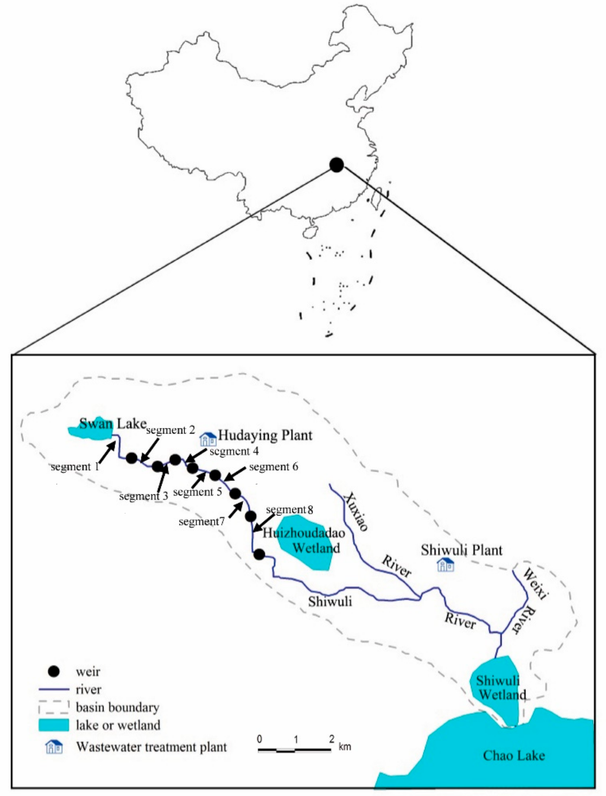
The Shiwuli River is a typical urban river. It is located in the urban area of Hefei City, Anhui Province. The river is 22.64 km long with a mean channel slope of 0.72%. The river width varies between 2 and 33 m. To enhance the river’s flood transfer ability, it has been channelized into a typical trapezoidal cross section with concrete walls. Eight weirs have been constructed in the river to store water and provide e-flows (Figure 1). In this research, we focus on the river segments influenced by weirs, and only river segments 1–8 are studied (the information about weirs and channels refers to Yin et al. [19]).

As a result of limited water input due to excessive withdrawals in upstream regions, the flows in the river are intermittent. To restore the river’s landscape and create a recreation site for citizens, the government plans to improve the water quality and secure e-flows in the river. The treated water from the Shiwuli wastewater treatment plant (with a treatment capacity of 25 × 10⁴ t/d, equivalent to 2.89 m³/s) and the Hudaying wastewater treatment plant (with a treatment capacity of 10 × 10⁴ t/d, equivalent to 1.16 m³/s) will be used to meet the e-flow requirements. The collected rainwater and water from Swan Lake will not serve as regular water sources. All industrial and domestic wastewater discharged into the river is expected to be treated by the two plants to achieve quality level IV (level IV is better than level V; level V is the water quality allowed for river scenery in China) in the released water according to the Chinese surface water standard [21]. In addition, to control non-point-source pollution caused by rain, many stormwater retention tanks will be constructed so that captured water can be treated to quality level IV before being released into the river. Planners believe that the wastewater control and treatment projects will control pollution releases into the river and produce a better river water quality than the allowed water release standard of V. Thus, the e-flows for pollutant dilution are negligible in this case.

The planned quality of water released from the two plants will meet the standard for level IV, which is better than the water quality (level V) allowed for the river. Part of the effluent (1.16 m³/s) from the Shiwuli wastewater treatment plant will first be transferred to the planned Huizhoudadao Wetland, located upstream of the Shiwuli plant, for further treatment, and will then be transferred immediately into the river downstream of Swan Lake, above the eight weirs. The effluent (1.16 m³/s) from the Hudaying plant will be released directly into the river channel to supply the e-flows.

2.2. Method Development

According to research done by Yin et al. [19], three e-flow scenarios are proposed in this research, corresponding to high, medium, and low hydrological connectivity. Under the high- and medium-connectivity scenarios, permanent hydrological connectivity is maintained, while under the low-connectivity scenario intermittent connectivity is ensured over time. A brief introduction to the method follows; for details about the method, see Yin et al. [19].

2.2.1. E-Flow Requirements under High Hydrological Connectivity

Algal blooms are common problems in urban rivers. Besides water quality, flow velocity is a key factor related to algal blooms. Thus, the high hydrological connectivity scenario tries to sustain the velocity of flows. The flow velocity is related to channel morphology and weir height, and these factors are not uniform among river segments. Thus, the flow velocities are also different in different river segments. The e-flow requirements in a river should be determined segment by segment. In this research, the river segments are divided according to the location of the weirs.

To reduce the possibility of algal blooms, the flow velocity should be maintained at a relatively high value of v₀. Here the flow velocity at the upstream side of the downstream weir is adopted to represent the velocity within a specified river segment [19]. The e-flow requirements can be determined using the following equations:

$$Q=\sigma \epsilon C_{d}b\sqrt{2g}{h}_0{}^{3/2}$$

(1)

$$h_0=\Delta h+\frac{a_0{v}^2}{2g}$$

(2)

$$v=\frac{Q}{[a+m(h+\Delta h\left)\right](h+\Delta h)},$$

(3)

where Q is the discharge required to ensure the specified flow velocity; σ is the submergence coefficient; ε is the lateral contraction coefficient; C_d is the discharge coefficient of weir flow; b is the weir length; g is the gravity acceleration coefficient; h₀ is the total head upstream of weir; Δh is the height of the water above the crest of the weir; a₀ is the kinetic energy correction factor; v is the flow velocity (i.e., v₀ in this research); a is the channel bottom width; m is the side slope coefficient; and h is the weir height.

2.2.2. E-Flow Determination under Medium Hydrological Connectivity

The longitudinal connectivity of material, energy, and information in rivers is a key requirement to maintain the ecological functions of rivers. Due to the blockage of dams or weirs, the longitudinal hydrological connectivity is often interrupted. Thus, the medium hydrological connectivity tries to ensure the hydraulic connectivity of river segments isolated by weirs.

In this research, Manning’s Equation, commonly used for open channel flow, is adopted to determine the required discharges. The lowest water depth in a river segment is set at no less than a specified value, i.e., 0.2 m in this research. Because the water depth at the upstream river section is commonly the lowest in a river segment, the discharge needed at this section is calculated as the required e-flow. Manning’s Equation is a function of channel velocity, flow area, and channel slope [22]:

$$Q=\frac{1}{n}{AR}^{2/3}\sqrt{S}$$

(4)

A = (a + hm)h,

(5)

where n is the Manning roughness coefficient; A is the channel cross section area covered by water; R is the hydraulic radius; and S is the slope of the channel.

2.2.3. E-Flow Determination under Low Hydrological Connectivity

Due to the continuous input of pollutants into rivers, the water quality in a river will decline, especially for channelized urban rivers with low biological degradation ability. The previous two hydrological connectivity scenarios could ensure relatively good water quality, but also require a great amount of water. Due to limited water availability, the low hydrological connectivity model seeks to further reduce the required water amount. Low hydrological connectivity tries to replace the impounded water within a channel segment under a specified periodicity, to ensure that the water quality is not too poor.

Under the low hydrological connectivity scenario, one flow management cycle is divided into two phases, i.e., a flow retention phase and a flow release phase. Based on the decline in water quality in channel segments, water should be replaced with a specified periodicity. Here the water storing time is set to T₀ based on the water quality and climate condition, and the flow release velocity is set to v₁:

Q = E/(T₀ + T₁)

(6)

T₁ = E/Av₁,

(7)

where E is the water volume within a river segment that could be stored; T₁ is the time required to release all water in a river segment; and v₁ is the given velocity for the release of stored water, which is set to 0.2 m/s to reduce algal blooms in this research, and could be changed accordingly.

2.3. Effect of Channel Morphology Changes

Due to the water blockage caused by weirs, the natural flow velocity decreases significantly. Subsequently, the problem of sedimentation and siltation is very common in rivers with weirs. The channel morphological changes caused by siltation will lead to changes in the elevation of the channel bottom and changes in the channel slope.

Due to the increased elevation of the channel bottom, the weir heights relative to the channel bottom will decrease, and Equation (3) could be revised as follows:

$$v=\frac{Q}{[a+m(h-se+\Delta h\left)\right](h-se+\Delta h)},$$

(8)

where se is the added siltation depth after weir construction.

In addition, the channel slope will also be changed, and thus Equation (4) could be revised as follows:

$$Q=\frac{1}{n}{\mathrm{AR}}^{2/3}\sqrt{S-ss},$$

(9)

where ss is the change in channel slope caused by siltation after weir construction.

Moreover, the water volume that could be stored within a river segment (E) will also change with changes in siltation depth. E can be determined easily based on the channel morphological information.

3. Results

As sediments are trapped by weirs, the channel morphology will change. In this paper we assume that siltation initially takes place near weirs (upstream), and then gradually expands upward. To explore the effects of morphological changes on e-flow requirements, the siltation depths are set to 0.1–0.5 m at increments of 0.1 m. The new e-flow requirements under the high hydrological connectivity scenario are listed in

Table 1. E-flow requirements (m³/s) for different river segments (SE) under the high hydrological connectivity scenario with a specified flow velocity of 0.1 m/s.

Siltation Depth (m)	SE 1	SE 2	SE 3	SE 4	SE 5	SE 6	SE 7	SE 8
0	2.63	2.51	1.61	3.11	2.32	1.02	6.02	5.03
0.1	2.45	2.40	1.45	2.88	2.16	0.85	5.70	4.82
0.2	2.37	2.31	1.35	2.77	2.03	0.71	5.38	4.53
0.3	2.29	2.23	1.25	2.65	1.90	0.58	5.05	4.24
0.4	2.21	2.14	1.15	2.54	1.77	0.44	4.73	3.95
0.5	2.12	2.05	1.05	2.43	1.64	0.30	4.41	3.66

(flow velocity = 0.1 m/s) and

Table 2. E-flow requirements (m³/s) for different river segments (SE) under the high hydrological connectivity scenario with a specified flow velocity of 0.2 m/s.

Siltation Depth (m)	SE 1	SE 2	SE 3	SE 4	SE 5	SE 6	SE 7	SE 8
0	5.23	5.11	3.21	6.21	4.62	2.02	13.02	11.83
0.1	5.17	5.07	3.11	6.09	4.61	1.86	12.16	10.30
0.2	5.01	4.89	2.90	5.86	4.34	1.58	11.49	9.69
0.3	4.83	4.71	2.69	5.62	4.07	1.29	10.81	9.08
0.4	4.66	4.53	2.48	5.39	3.80	0.99	10.13	8.47
0.5	4.49	4.35	2.27	5.16	3.52	0.69	9.45	7.86

(flow velocity = 0.2 m/s). The tables show that the e-flow requirements are significantly impacted by the channel morphological changes for all river segments. With the increased depth of siltation, the e-flow requirements under the high hydrological connectivity scenario will decrease. This indicates that if the water resources available for e-flow supply are too limited to meet the e-flow requirements, modifying the channel morphology is a potential solution.

In addition, the change ratio of e-flow requirements under the high hydrological connectivity scenario is listed in

Table 3. Reduction ratio of e-flow requirement for different river segments (SE) under the high hydrological connectivity scenario with a specified flow velocity of 0.1 m/s.

Siltation Depth (m)	SE 1	SE 2	SE 3	SE 4	SE 5	SE 6	SE 7	SE 8
0.1	6.75%	4.47%	9.87%	7.50%	6.87%	16.72%	5.28%	4.15%
0.2	9.87%	7.90%	16.07%	11.08%	12.48%	29.92%	10.66%	9.92%
0.3	12.99%	11.33%	22.27%	14.67%	18.10%	43.22%	16.04%	15.70%
0.4	16.12%	14.77%	28.49%	18.26%	23.72%	56.64%	21.43%	21.50%
0.5	19.24%	18.20%	34.73%	21.85%	29.36%	70.26%	26.83%	27.30%

and

Table 4. Reduction ratio of e-flow requirement for different river segments (SE) under the high hydrological connectivity scenario with a specified flow velocity of 0.2 m/s.

Siltation Depth (m)	SE 1	SE 2	SE 3	SE 4	SE 5	SE 6	SE 7	SE 8
0.1	1.05%	0.85%	3.17%	1.98%	0.12%	7.84%	6.60%	12.96%
0.2	4.30%	4.34%	9.67%	5.70%	6.00%	22.00%	11.78%	18.09%
0.3	7.55%	7.84%	16.18%	9.43%	11.90%	36.32%	16.97%	23.22%
0.4	10.81%	11.34%	22.72%	13.16%	17.81%	50.86%	22.18%	28.37%
0.5	14.07%	14.85%	29.29%	16.90%	23.74%	65.73%	27.40%	33.54%

. The change ratio of e-flow requirements varies for different river segments. Among them, the change ratio for river segment 6 is the largest, while the change ratio for segment 2 is the smallest. The e-flow change ratio is closely related to the weir height. The height of weir 6 is the lowest, at only 0.7 m. Thus, a siltation depth of 0.1 m is significant compared with the weir height.

The change ratio of e-flow requirements under a flow velocity of 0.1 m/s or 0.2 m/s is also different. The change ratio at a low flow velocity is obviously greater than that under a high flow velocity. For example, under a flow velocity of 0.1 m/s, the e-flow decreases by 6.75% and 16.72% for river segments 1 and 6 with a siltation depth of 0.1 m, respectively, while under a flow velocity of 0.2 m/s, the e-flow only decreases by 1.05% and 7.84% for river segments 1 and 6 with a siltation depth of 0.1 m, respectively. Thus, modifying channel morphology to aid e-flow supply is more effective under low flow velocity requirements.

In terms of medium hydrological connectivity, siltation also has obvious effects on e-flow requirements (

Table 5. E-flow requirements (m³/s) for different river segments (SE) under the medium hydrological connectivity scenario.

Siltation Depth (m)	SE 1	SE 2	SE 3	SE 4	SE 5	SE 6	SE 7	SE 8
0	0.67	1.34	1.01	1.34	1.12	0.52	1.14	1
0.1	0.59	1.32	0.97	1.29	1.08	0.42	1.10	0.96
0.2	0.50	1.30	0.94	1.25	1.05	0.30	1.05	0.92
0.3	0.39	1.29	0.90	1.20	1.01	0.00	1.00	0.88
0.4	0.24	1.27	0.86	1.15	0.98	0.00	0.95	0.84
0.5	0.00	1.25	0.82	1.09	0.94	0.00	0.90	0.80

and

Table 6. Reduction ratio of e-flow requirement for different river segments (SE) under the medium hydrological connectivity scenario.

Siltation Depth (m)	SE 1	SE 2	SE 3	SE 4	SE 5	SE 6	SE 7	SE 8
0.1	12.07%	1.37%	3.51%	3.57%	3.31%	18.31%	3.83%	4.11%
0.2	25.27%	2.65%	7.02%	7.08%	6.38%	42.24%	7.92%	7.87%
0.3	41.38%	3.94%	10.67%	10.73%	9.55%	100.00%	12.21%	11.79%
0.4	64.10%	5.24%	14.47%	14.53%	12.84%	100.00%	16.71%	15.90%
0.5	100.00%	6.57%	18.45%	18.50%	16.26%	100.00%	21.48%	20.22%

). With an increase in siltation depth, the e-flow requirements decrease. For some river segments, the e-flow requirements even become 0. For example, when the siltation depth exceeds 0.3 m, the e-flow requirements for river segment 6 become 0. This means that no continuous water input is required to maintain hydrological connectivity (the evaporation and seepage are not considered) after the water level exceeds 0.2 m. This is because the channel slope for river segment 6 is very low. When the siltation depth increases by 0.3 m, the channel slope becomes nearly 0 and thus the flow velocity decreases to nearly 0.

Besides the significant changes in e-flow requirements in river segments 6 and 1, the change ratio in segments 7 and 8 also exceeds 20%. However, the change ratio of e-flow requirements for river segment 2 is very limited. It is only 6.57% when the siltation depth increases by 0.5 m. This is due to the highest channel slope being in river segment 2.

Under the low hydrological connectivity regime, e-flow requirements also decrease with an increase in siltation depth. In this research the water storing time T₀ is set to three days. The e-flow reduction ratio for segments 6‒8 is the greatest, higher than 70%. The reduction ratio for segments 1 and 4 is the lowest, no more than 30% (

Table 7. E-flow requirements (m³/s) for different river segments (SE) under the low hydrological connectivity scenario.

Siltation Depth (m)	SE 1	SE 2	SE 3	SE 4	SE 5	SE 6	SE 7	SE 8
0	1.03	0.13	0.09	0.17	0.24	0.14	0.49	0.64
0.1	1.00	0.12	0.08	0.16	0.21	0.12	0.42	0.55
0.2	0.96	0.11	0.07	0.15	0.19	0.09	0.35	0.46
0.3	0.93	0.09	0.05	0.14	0.16	0.07	0.28	0.37
0.4	0.89	0.08	0.04	0.13	0.13	0.04	0.21	0.27
0.5	0.86	0.07	0.03	0.12	0.11	0.02	0.14	0.18

and

Table 8. Reduction ratio of e-flow requirement for different river segments (SE) under the low hydrological connectivity scenario.

Siltation Depth (m)	SE 1	SE 2	SE 3	SE 4	SE 5	SE 6	SE 7	SE 8
0.1	3.37%	9.48%	13.84%	5.51%	11.12%	17.76%	14.41%	14.28%
0.2	6.74%	18.95%	27.67%	11.02%	22.24%	35.52%	28.83%	28.56%
0.3	10.12%	28.43%	41.51%	16.53%	33.36%	53.28%	43.24%	42.84%
0.4	13.49%	37.91%	55.35%	22.04%	44.48%	71.04%	57.66%	57.12%
0.5	16.86%	47.39%	69.18%	27.55%	55.61%	88.80%	72.07%	71.40%

).

Table 1, Table 2, Table 3, Table 4, Table 5, Table 6, Table 7 and Table 8 also show that the sensitivity of e-flow requirements to morphological changes is different under high, medium, and low hydrological connectivity. Under the high hydrological connectivity scenario, river segment 1 is the least sensitive and the sensitivity sequence is segment 6 > segment 8 > segment 3 > segment 7 > segment 5 > segment 4 > segment 2 > segment 1 for a planned flow velocity of 0.2 m/s. while under the medium hydrological connectivity scenario, river segment 2 is the least sensitive, and the sensitivity sequence is segment 6 > segment 1 > segment 7 > segment 8 > segment 3 > segment 4 > segment 5 > segment 2; under the low hydrological segment, the sensitivity sequence is segment 6 > segment 7 > segment 8 > segment 3 > segment 5 > segment 2 > segment 4 > segment 1. The difference in the sensitivity sequences is due to different primary influence factors. For high hydrological connectivity, the relative weir height is the primary influence factor, while for medium hydrological connectivity the channel slope is the primary influence factor, and for low hydrological connectivity all the channel morphological characteristics, including channel width, length, and slope, exert an influence.

4. Discussion

4.1. Tradeoff between Flood Control and E-Flow Supply

Although siltation could reduce the e-flow requirements, which is positive in terms of sufficient e-flow, siltation is negative for flood control. For the Shiwuli River, the design standard is a 100-year flood.

Table 9. Flood control ability (m³/s) for different river segments (SE) under different siltation depths.

Siltation Depth (m)	SE 1	SE 2	SE 3	SE 4	SE 5	SE 6	SE 7	SE 8
0	88.62	99.27	109.21	116.20	132.97	153.00	172.91	187.84
0.1	84.20	94.54	103.88	110.29	126.16	145.84	159.32	174.83
0.2	79.87	89.88	98.64	104.47	119.47	138.79	146.10	162.13
0.3	75.60	85.31	93.48	98.77	112.90	131.86	133.27	149.76
0.4	71.42	80.81	88.43	93.17	106.45	125.05	120.84	137.72
0.5	67.32	76.40	83.46	87.69	100.14	118.35	108.82	126.02

lists the flow magnitude that the river can tolerate under different siltation depths. With an increase in siltation depth, the maximum flows allowed that will not lead to flooding decrease. When the siltation depth increases to 0.5 m, the reduction ratio of flood magnitude allowed exceeds 20% for all river segments (

Table 10. Reduction ratio of flood control ability for different river segments (SE) under different siltation depths.

Siltation Depth (m)	SE 1	SE 2	SE 3	SE 4	SE 5	SE 6	SE 7	SE 8
0.1	4.98%	4.77%	4.89%	5.09%	5.13%	4.68%	7.86%	6.93%
0.2	9.88%	9.46%	9.69%	10.09%	10.16%	9.29%	15.50%	13.69%
0.3	14.69%	14.07%	14.40%	15.00%	15.10%	13.82%	22.92%	20.28%
0.4	19.41%	18.60%	19.03%	19.82%	19.94%	18.27%	30.11%	26.69%
0.5	24.04%	23.04%	23.58%	24.54%	24.70%	22.64%	37.06%	32.91%

). Especially for segment 7, the reduction ratio is 37.06%. Segment 7 should be given the highest priority for siltation control to avoid flood disasters.

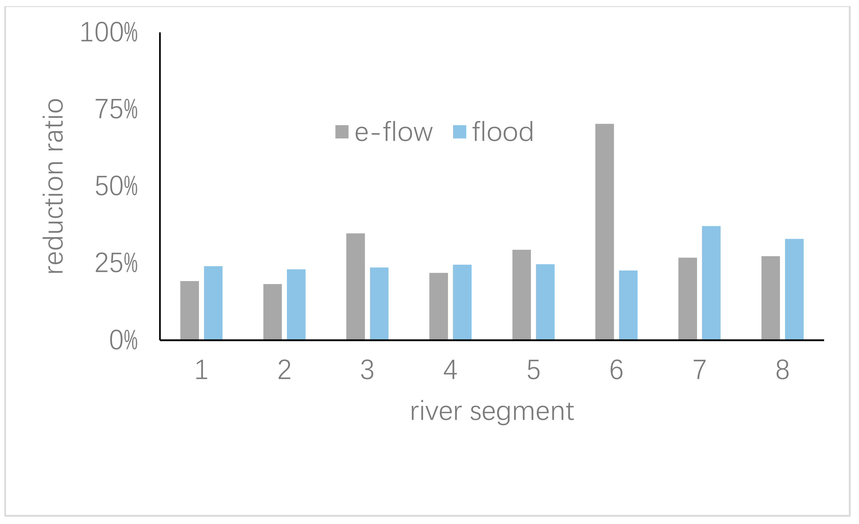
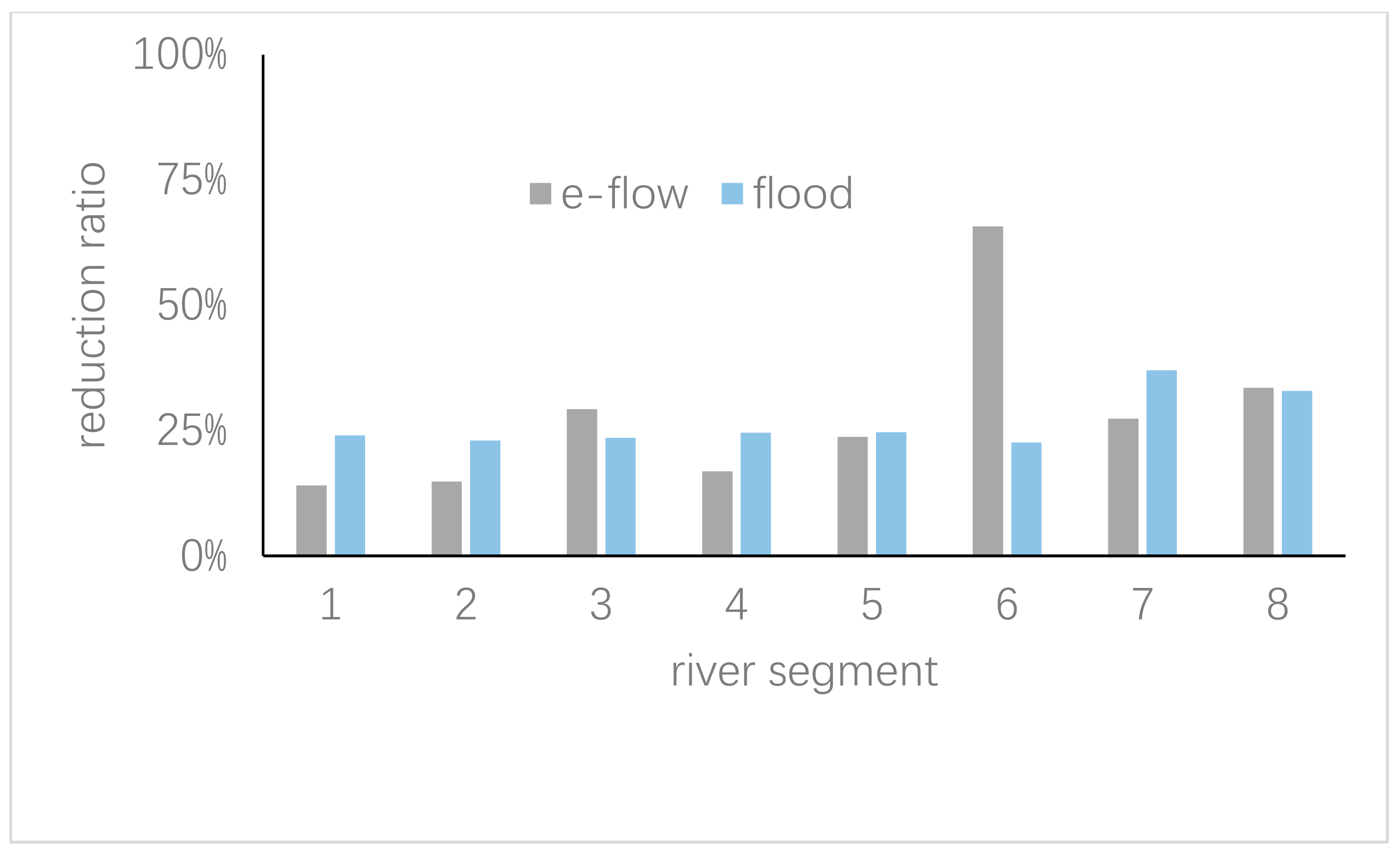
The benefits of siltation for e-flow supply and flood control are compared in Figure 2, Figure 3, Figure 4 and Figure 5. When the planned flow velocity for e-flow requirements is 0.1, the e-flow reduction ratio in river segments 3, 5, and 6 is greater than the flood reduction ratio; in segments 3 and 6 only, the e-flow reduction ratio is greater than the flood reduction ratio. Thus, if siltation is used to satisfy the e-flow requirements, segments 3 and 6 should be the primary area. The flood reduction ratios for segments 1, 2, 4, and 7 are greater than the e-flow reduction ratio under a planned flow velocity 0.1 m/s or 0.2 m/s. In these four river segments, dredging has a more significant effect.

Under the medium hydrological connectivity scenario, the comparison results between e-flow supply and flood control are different from those under the high hydrological connectivity scenario. The e-flow reduction ratio in segments 1 and 6 is obviously greater than the flood reduction ratio, while in the other river segments the e-flow reduction ratio is lower. Thus, if siltation is used to satisfy the e-flow requirements, segments 1 and 6 should be the primary area to allow siltation for e-flow satisfaction under the medium hydrological scenario.

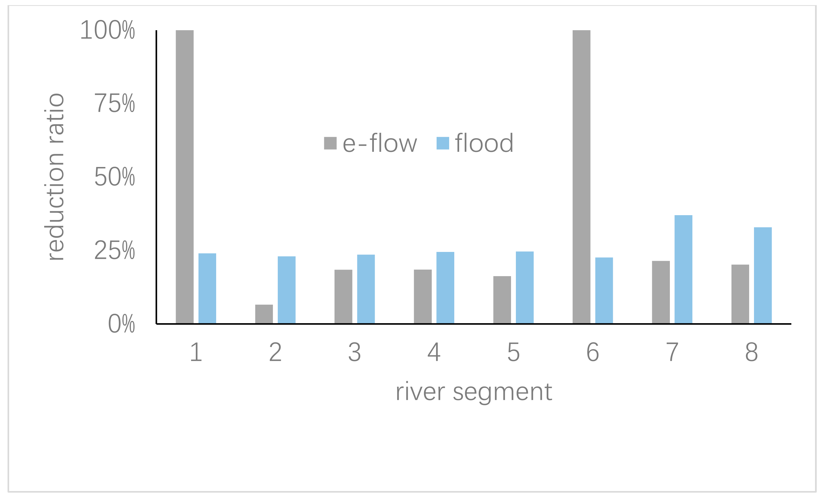
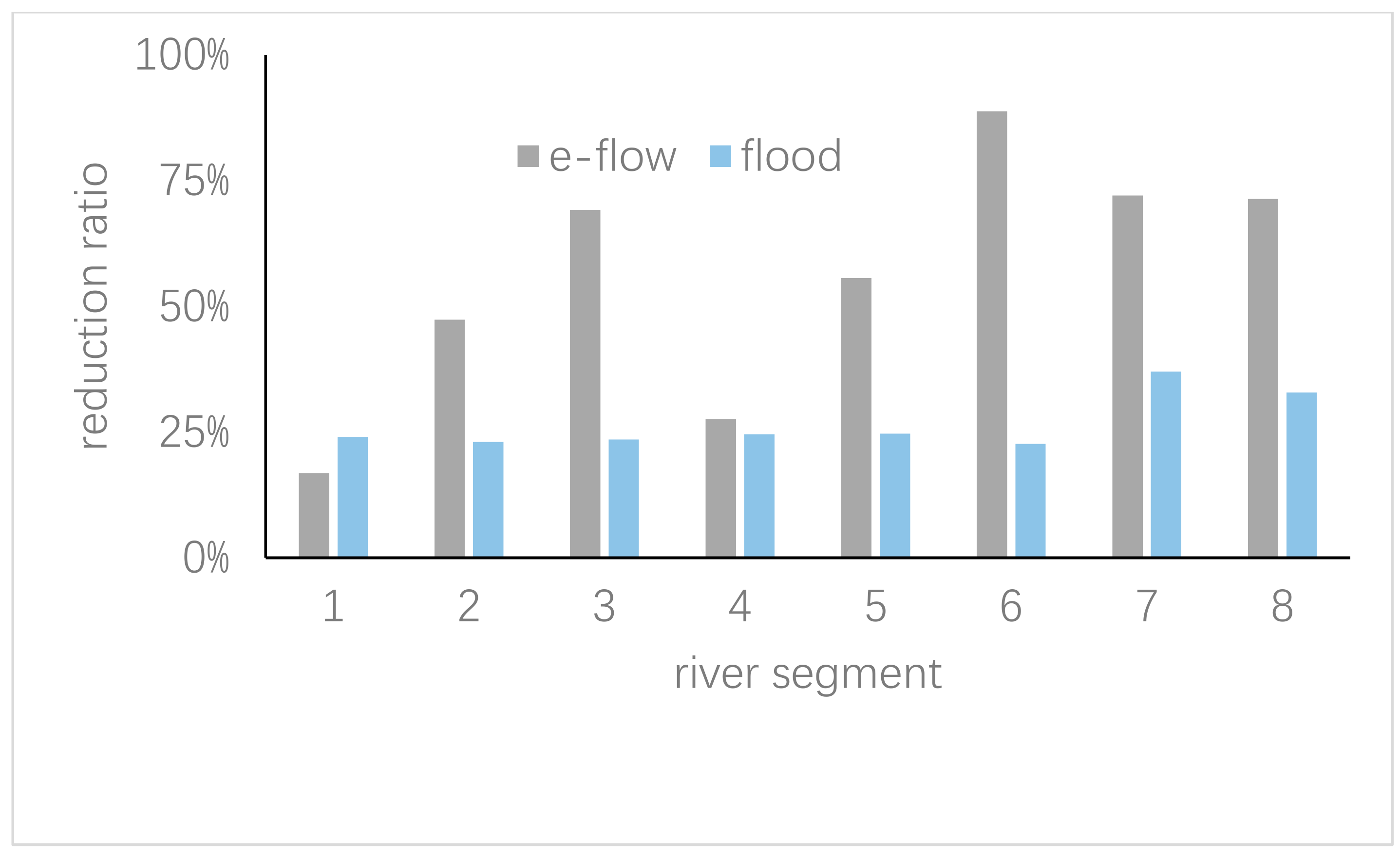
Under the low hydrological connectivity scenario, the comparison results between e-flow supply and flood control are obviously different from those under the high and medium hydrological connectivity scenarios. The e-flow reduction ratio in segments 2, 3, 5, 6, 7, and 9 is obviously greater than the flood reduction ratio. In these segments, siltation may be a potential solution to satisfy the e-flow requirements. In comparison, the flood reduction ratio is greater than the e-flow reduction ratio in segment 1, and thus, dredging should be adopted in this segment.

Due to the positive effects of siltation on e-flow supply, the timing, frequency, and volume of dredging should be further optimized. Dredging could begin before the flood season. A 100-year flood is the design standard for the Shiwuli River. The standard is very high and such large floods represent a very low possibility. A reliable flood prediction model is valuable to balance the needs of flood control and e-flow supply. With a reliable flood prediction model, river managers could determine the frequency and volume of dredging. If a specific flood risk is allowed, the dredging frequency and volume could be reduced to some degree.

4.2. E-Flow Comparison under Different E-Flow Assessment Methods

In this research, following the new e-flow assessment method established by Yin et al. [19], we explore the influence of channel morphological changes on e-flow requirements. However, as mentioned in the introduction, besides the method by Yin et al. [19], hydrological, hydraulic rating, habitat simulation, and holistic methods are four commonly used method types to determine e-flows. These four methods usually assume that the channel morphology does not change. It is necessary to further explore the influence of channel morphological changes on e-flow requirements under the four methods.

The hydrological methods are based on hydrological data. The underlying assumption is that hydrological data, i.e., historical flow data, can effectively reflect the characteristics of a river. However, the historical flow data cannot reflect continuous changes in channel morphology. If hydrological methods are to be adopted in future research (when only hydrological data are available), the latest flow data, which correspond to the new channel morphology, should be used to determine e-flows.

Morphological data are necessary for the hydraulic rating, habitat simulation, and holistic methods. In hydraulic rating methodologies, hydraulic variables, such as wetted perimeter, will be determined. These hydraulic variables are closely related to river channel morphology. The e-flow results under the hydraulic rating methodologies can reflect the influence of river morphological changes. Although the e-flow results under the habitat simulation and holistic methods are influenced by changes in river morphology, in real-world research the river morphology is usually assumed to be fixed to reduce the complexity of e-flow assessment and management. To reduce the deviation of e-flow results, it is suggested that we update the e-flow results every few years, especially for rivers with a high sediment concentration.

5. Conclusions

Sustaining e-flows, as an essential measure to maintain the health of urban rivers, has been adopted widely. However, previous research on e-flow requirements has usually assumed that the river morphology is fixed, and has not considered the influence of morphological changes caused by siltation. Because siltation is inevitable due to the flow velocity decrease caused by weirs, this research seeks to explore the influence of siltation on e-flow requirements. The Shiwuli River is adopted as a case study, and the following conclusions are drawn.

• The river morphological changes can significantly influence the e-flow requirements. An increase in siltation depth will lead to a decrease in e-flow requirements.
• The sensitivity of e-flow requirements to morphological changes varies among river segments and hydrological connectivity. The sensitivity is related to the channel width, length, and slope as well as the weir heights.
• Despite the positive effects of siltation on e-flow supply, the negative effects on flood control are also obvious. The river segments that should be given high priority for dredging are identified based on the balance of requirements between e-flow supply and flood control.
• Morphological changes will lead to obvious errors in e-flow results under different e-flow assessment methods, especially under the hydrological methods. It is suggested that we update e-flow results every few years based on new morphological data.

References

- Postel, S.L.; Daily, G.C.; Ehrlich, P.R. Human appropriation of renewable freshwater. Science 1996, 271, 785–788. [Google Scholar] [CrossRef]
- Postel, S.L. Water for food production: Will there be enough in 2025? BioScience 1998, 48, 629–637. [Google Scholar] [CrossRef]
- Rosenberg, D.M.; McCully, P.; Pringle, C.M. Global-scale environmental effects of hydrological alterations: Introduction. BioScience 2000, 50, 746–751. [Google Scholar] [CrossRef]
- Nilsson, C.; Reidy, C.A.; Dynesius, M.; Revenga, C. Fragmentation and flow regulation of the world’s large river systems. Science 2005, 308, 405–408. [Google Scholar] [CrossRef] [PubMed]
- Ramos, V.; Formigo, N.; Maia, R. Environmental flows under the WFD implementation. Water Resour. Manag. 2018, 32, 5115–5149. [Google Scholar] [CrossRef]
- King, J.; Brown, C.; Sabet, H. A scenario-based holistic approach to environmental flow assessments for rivers. River Res. Appl. 2003, 19, 619–639. [Google Scholar] [CrossRef]
- Dunbar, M.J.; Gustard, A.; Acreman, M.C.; Elliott, C.R.N. Review of Overseas Approaches to Setting River Flow Objectives; Environment Agency R&D Technical Report W6B(96)4; Institute of Hydrology: Wallingford, UK, 1998. [Google Scholar]
- Prewitt, C.G.; Carlson, C.A. Evaluation of Four Instream Flow Methodologies Used on the Yampa and White Rivers, Colorado; Biological Sciences Series Number Two; Bureau of Land Management: Denver, CO, USA, 1980.
- Tharme, R.E. Review of International Methodologies for the Quantification of the Instream Flow Requirements of Rivers. Water Law Review Final Report for Policy Development for the Department of Water Affairs and Forestry, Pretoria; Freshwater Research Unit, University of Cape Town: Cape Town, South Africa, 1996. [Google Scholar]
- Ward, J.A.; Stanford, J.A. The ecology of regulated streams: Past accomplishments and directions for future research. In Regulated Streams: Advances in Ecology; Craig, J.F., Kemper, J.B., Eds.; Plenum Press: New York, NY, USA, 1987; pp. 391–409. [Google Scholar]
- Petts, G.E. Perspectives for ecological management of regulated rivers. In Alternatives in Regulated River Management; Gore, J.A., Petts, G.E., Eds.; CRC Press: Boca Raton, FL, USA, 1989; pp. 3–24. [Google Scholar]
- Tharme, R.E. An overview of environmental flow methodologies, with particular reference to South Africa. In Environmental Flow Assessments for Rivers: Manual for the Building Block Methodology; King, J.M., Tharme, R.E., De Villiers, M.S., Eds.; Water Research Commission Technology Transfer Report No. TT131/00; Water Research Commission: Pretoria, South Africa, 2000; pp. 15–40. [Google Scholar]
- Arthington, A.H. Brisbane river trial of a flow restoration methodology (FLOWRESM). In Water for the Environment: Recent Approaches to Assessing and Providing Environmental Flows, Proceedings of AWWA Forum, Arthington, Brisbane, Australia, April 1998; Zalucki, J.M., Ed.; AWWA: Brisbane, Australia, 1998; pp. 35–50. [Google Scholar]
- Morley, S.A.; Karr, J.R. Assessing and restoring the health of urban streams in the Puget Sound Basin. Conserv. Biol. 2002, 16, 1498–1509. [Google Scholar] [CrossRef]
- Chin, A. Urban transformation of river landscapes in a global context. Geomorphology 2006, 79, 460–487. [Google Scholar] [CrossRef]
- Chang, F.J.; Tsai, Y.H.; Chen, P.A.; Coynel, A.; Vachaud, G. Modeling water quality in an urban river using hydrological factors—Data driven approaches. J. Environ. Manag. 2015, 151, 87–96. [Google Scholar] [CrossRef] [PubMed]
- Willis, A.D.; Campbell, A.M.; Fowler, A.C.; Babcock, C.; Howard, J.; Deas, M.L.; Nichols, A.L. Instream flows: New tools to quantify water quality conditions for returning adult chinook salmon. J. Water Resour. Plan. Manag. 2016, 142, 04015056. [Google Scholar] [CrossRef]
- Jia, H.; Ma, H.; Wei, M. Calculation of the minimum ecological water requirement of an urban river system and its deployment: A case study in Beijing central region. Ecol. Mode 2011, 222, 3271–3276. [Google Scholar] [CrossRef]
- Yin, X.A.; Yang, Z.F.; Zhang, E.Z.; Xu, Z.H.; Cai, Y.P.; Yang, W. A new method of assessing environmental flows in channelized urban rivers. Engineering 2018, 4, 590–596. [Google Scholar] [CrossRef]
- Tharme, R.E. A global perspective on environmental flow assessment: Emerging trends in the development and application of environmental flow methodologies for rivers. River Res. Appl. 2003, 19, 397–441. [Google Scholar] [CrossRef]
- Ministry of Environmental Protection 528 of China (MEP). Environmental Quality Standard for Surface Water (GB 3838-2002); Ministry of Environmental Protection: Beijing, China, 2002. [Google Scholar]
- Niazkar, M.; Afzali, S.H. Optimum design of lined channel sections. Water Resour. Manag. 2015, 29, 1921–1932. [Google Scholar] [CrossRef]
Figure 1.
Location of the Shiwuli River and its weirs.
Figure 2.
Comparison of reduction ratios between e-flow requirement and flood control ability under the high hydrological connectivity scenario (specific flow velocity = 0.1 m/s) with a siltation depth equal to 0.5 m.
Figure 3.
Comparison of reduction ratios between e-flow requirement and flood control ability under the high hydrological connectivity scenario (specific flow velocity = 0.2 m/s) with a siltation depth equal to 0.5 m.
Figure 4.
Comparison of reduction ratios between e-flow requirement and flood control ability under the medium hydrological connectivity scenario with a siltation depth equal to 0.5 m.
Figure 5.
Comparison of reduction ratios between e-flow requirement and flood control ability under the low hydrological connectivity scenario with a siltation depth equal to 0.5 m.