Rice Irrigation Schedule Optimization Based on the AquaCrop Model: Study of the Longtouqiao Irrigation District

Abstract

As a crop with high water consumption, rice is an important measure of efforts to improve agricultural irrigation efficiency and alleviate the contradiction between the supply and demand of agricultural water resources. This paper takes the Longtouqiao irrigation district, in the hinterland of the Sanjiang Plain, a major rice-producing area in northern China, as an example, and the AquaCrop crop growth model and entropy-cloud model are jointly used to develop a rice irrigation schedule optimization model based on three kinds of typical rainfall years. Different irrigation schemes are established and evaluated by using the model built based on images. The results showed that the yield’s normalized root mean square error (NRMSE) value of the AquaCrop model was 9.949% (< 10%) after calibration, and the our model results showed a good agreement with observed data, which indicated that the calibrated model was suitable for rice growth simulation in the research area. For the same irrigation water amount, rice was irrigated to a great extent at the tillering stage, and a small amount of irrigation water at the regreening stage of rice could improve rice yield. During irrigation, rice production can also be promoted by regulating the irrigation amount according to the rainfall in each growth period, and the optimal irrigation water amount can be controlled between 20 and 60 mm each time. Under the three typical annual scenarios of dry, normal and wet years, the respective optimal quantification results for the field capacity, total irrigation water amount and irrigation times in the rice growth period to attain the optimal irrigation effect were 25%, 425 mm, and 17 times, respectively; 25%, 450 mm, and 14 times; respectively, and 25%, 425 mm, and 17 times, respectively. The research results can provide a decision-making basis for water-saving measures and efficient rice irrigation water management.

1. Introduction

As a major irrigated country in the world, over 70% of China’s grain, 80% of its cotton and 90% of its vegetables come from irrigation agriculture [1]. Rice is the second largest grain crop in the world in terms of area and total yield. Rice consumes 50% of the irrigation water and 63% of fertilizers [2,3]. However, China is experiencing a water shortage and inefficiently manages the water use in agriculture [4,5,6]. Therefore, developing a reasonable rice irrigation schedule under the condition of insufficient irrigation is of great significance to improve the agricultural water use efficiency [7].

For more than half a century, scholars at home and abroad have conducted much research on irrigation schedule optimization. Hall, Dudley and De Lucia [8,9,10] adopted a dynamic programming model, setting runoff or rainfall as random variables to develop a crop irrigation schedule. On the basis of the knowledge gained from foreign research experience, China’s irrigation schedule research has developed rapidly. A dynamic programming model was used to optimize the irrigation schedule at the rice growing stage [11,12,13]. Tian [14] constructed a decision system based on a geographic information system (GIS) and genetic algorithms to optimize the combined irrigation schedule. Based on the Jensen model, Yu Zhijing [15] applied the improved non-dominated sorting genetic algorithm (NSGA-II) to obtain the irrigation date and irrigation amount of winter wheat and summer corn. Osama [16] established a linear optimization model for the annual net income of the region that took into account the spatial change in crops, irrigation water demand, crop yield and grain reserve. Dang [17] took a typical rice irrigation schedule as the research object, established the optimal coupling model of hydrological irrigation, and deduced the corresponding irrigation strategy. Li [18,19] adopted the ILMP (interval linear multi-objective programming) and AWEFSM (Agricultural Water-Energy-Food Sustainable Management) models to determine the water–energy–food strategy under uncertain conditions and provided insights into the tradeoff of water management. Liu Xiao [20] analyzed the optimal planting structure under different conditions using the Monte Carlo simulation method. The above crop simulation model based on the water balance and water production function is based on a large number of field experimental data analyses and calculations using empirical equations, and it is difficult to distinguish the influences of different field measures on crop growth processes from the mechanism. Compared with the traditional water production function method, the crop growth model can more comprehensively describe the processes of crop growth and development. Among these models, the AquaCrop model, which can accurately simulate farmland water balance and crop growth, is widely used in research on the impacts of water and fertilizers on soil-to-crop systems, and scholars in different countries have applied the model successively [21,22,23,24] to winter wheat, soybean, sunflower, rice and other crops [25,26]. However, the application of the AquaCrop model in rice growth simulation and irrigation water optimization is not widely studied at present. Most of the studies take the irrigation water amount, yield or water productivity (WP) as a single optimization objective, and little consideration is given to displacement while the main way of irrigation loss, paddy drainage, is an important index to measure the emission reduction in paddy fields. However, there are few irrigation schedules that take irrigation water, drainage and yield into consideration.

Based on the above problems, taking the Longtouqiao irrigation district in the Sanjiang Plain as an example, a crop irrigation schedule optimization method based on field observations and scenario simulations was proposed. Through the AquaCrop crop growth model, the optimal irrigation schedule model under multiple irrigation scenarios with different precipitation years was established to determine the best irrigation mode and the optimal irrigation amounts and times. The results of this model are used to guide rice production under the water-saving conditions in this area and play a theoretical guiding role in the improvement of the paddy field environment in the Sanjiang Plain area, China, and, thus, this model has an important role in the agricultural yield increase and water-saving measures in this area.

2. Materials and Methods

2.1. Study Area

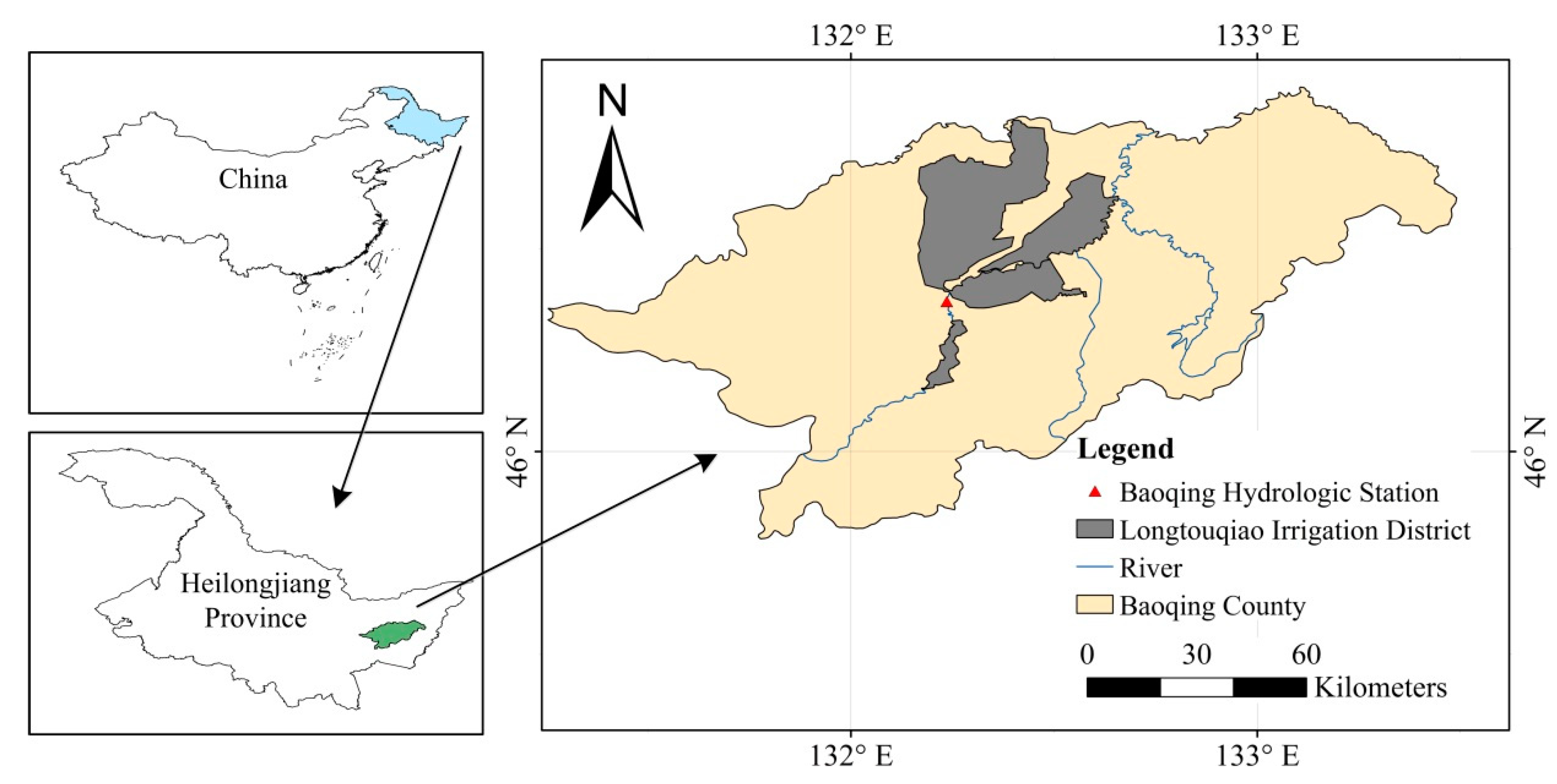
The Longtouqiao irrigation district is located in the middle and upper reaches of the Naoli River in the Sanjiang Plain, Heilongjiang Province, China. The administrative divisions within the irrigation district include 6 townships of Baoqing County, a second division of 597 state farms, and a third division of 853 state farms. The irrigation district has a maximum width of 28 km and a maximum length of 58 km. The geographical position is 129°31′–132°29′ E and 46°22′–48°05′ N. The study area position is shown in Figure 1. The irrigation district belongs to the mesothermal zone with a continental monsoon climate, and the soil is clay. The minimum monthly average temperature is −21.5 °C, the maximum monthly average temperature is 29.8 °C, and the average annual temperature is 3.2 °C. The average annual rainfall is 522 mm, mainly from June to September. The frost-free period is 145 d, and the annual average sunshine hours are 6.7 h. The control area is 4.97 × 10⁴ ha, the current cultivated area is 4.15 × 10⁴ ha, the designed irrigation area is 2.90 × 10⁴ ha, and the current irrigation area is 1.89 × 10⁴ ha, all of which are paddy fields. Among these areas, the surface water irrigation area is 1.55 × 10⁴ ha, and the groundwater irrigation area is 0.34 × 10⁴ ha. In The Plan for Supporting Facilities and Water-Saving Reconstruction in Large Irrigated Districts Across the Country approved by the Ministry of Water Resources in 2001, the Longtouqiao irrigation district is one of the 19 large irrigation districts in Heilongjiang Province included. The field data needed to calibrate the AquaCrop model were derived from the literature [27]; the required meteorological data were obtained through the China Meteorological Data Service Center (CMDC) (http://data.cma.cn/en), the national meteorological data network; and the required soil data were obtained from an experimental report of the irrigated areas.

2.2. AquaCrop Model and Parameters

The AquaCrop model [28] is a model to describe the structure of a continuous soil–crop–atmosphere system. This model is a water-driven model, and the response of the aboveground crop productivity to soil water is mainly realized by the soil water stress coefficient (K_s). Through roots, K_s affects leaf expansion, senescence and stomatal conductance and then affects the transpiration and biomass accumulation processes of crops. K_s can also impact the harvest index, which in turn affects the yield. Therefore, the output of this model mainly includes the following four parts: canopy coverdevelopment, biomass accumulation and soil moisture content changes during the crop growth period, and final rice yield. The core idea of the AquaCrop model is the D-K model proposed by Doorernbos and Kassam in 1979 [29]. On this basis, the AquaCrop model distinguishes soil evaporation from crop transpiration by the canopy coverage and then calculates the aboveground biomass by transpiration and normalized water production efficiency and controls the final yield by the harvest index. Thus, the relationship between the crop yield and transpiration is as follows:

B = WP* × ΣT

(1)

Y₀ = HI × B

(2)

where B is the aboveground biomass, t/hm²; WP* is the water production efficiency of the biomass (the normalized water production efficiency is obtained by normalizing the carbon dioxide concentration according to the different water production efficiency values), t/(hm² · mm); T is the daily transpiration, mm/day; Y₀ is the crop yield, kg/ha; and HI is the harvest index.

The AquaCrop model [30] provides the characteristics and related growth parameters of typical rice crops, but the relevant parameters of the model need to be corrected for specific areas. According to field observation data, the basic data required by the model, including meteorological data, soil data, irrigation schedule, field management measures and original soil moisture content, were determined, and the parameters of the model were calibrated and verified to obtain the crop growth model applicable to the research area.

2.3. Irrigation Scenario Setting and Optimization Model

2.3.1. Irrigation Scenario Simulation Setting

In this paper, when carrying out irrigation schedule optimization, the Pearson-III type curve is adopted to conduct frequency analysis on the rainfall data from 1956 to 2018 of Baoqing County. The annual rainfall with a guaranteed rainfall rate of 25% (in wet years), 50% (in normal years) and 75% (in dry years) is 593.6 mm, 498.3 mm and 419 mm, respectively, and the corresponding years are 2013, 1997 and 1999, respectively. During the experiment, too little water in the soil (soil moisture content of 70%) inhibited tillering. When simulating irrigation scenarios, four main factors are emphatically considered: irrigation water amount, number of irrigations, irrigation time and field capacity (FC). The irrigation water quantity interval is (120,1000) mm, and the irrigation frequency interval is [6,25] times. The field moisture capacity is set from 20–45% according to the soil type. In this paper, 28 irrigation schedule scenarios are defined, and the irrigation time and irrigation water amount of each scenario are shown in

Table 1. Amount of irrigation and times ofiIrrigation under each scenario.

Treatment	Regreening Stage		Tillering Stage		Jointing Stage		Heading Stage		Milky Stage		Irrigation Schedule
	Amount of Irrigation (mm)	Times of Irrigation	Amount of Irrigation (mm)	Times of Irrigation	Amount of Irrigation (mm)	Times of Irrigation	Amount of Irrigation (mm)	Times of Irrigation	Amount of Irrigation (mm)	Times of Irrigation	Amount of Irrigation (mm)	Times of Irrigation
T1	0	0	80	4	20	1	20	1	0	0	120	6
T2	0	0	100	5	0	0	20	1	20	2	140	8
T3	20	1	70	3	30	1	40	1	30	1	190	7
T4	60	3	120	4	30	1	40	1	30	1	276	10
T5	60	3	120	6	80	4	60	3	0	0	320	16
T6	30	1	180	9	30	1	50	2	0	0	330	13
T7	0	0	180	9	80	4	60	3	30	1	350	17
T8	60	3	150	6	80	4	60	3	0	0	350	16
T9	60	3	195	8	40	2	100	4	30	1	425	18
T10	60	3	195	8	100	3	40	2	30	1	425	17
T11	270	9	155	5	0	0	0	0	0	0	425	14
T12	0	0	425	9	0	0	0	0	0	0	425	9
T13	70	2	200	6	80	2	60	2	40	2	450	14
T14	0	0	450	13	0	0	0	0	0	0	450	13
T15	70	1	200	6	80	2	60	1	40	1	450	11
T16	30	1	240	7	80	2	60	2	40	2	450	14
T17	110	3	160	5	80	2	60	2	40	2	450	14
T18	70	2	240	7	80	2	60	2	0	0	450	13
T19	70	2	250	5	100	2	30	1	0	0	450	10
T20	70	2	250	8	30	1	80	2	20	1	450	14
T21	80	2	240	4	100	2	30	1	0	0	450	9
T22	100	3	210	5	80	2	30	1	30	1	450	12
T23	100	3	200	6	60	1	30	1	60	1	450	12
T24	110	3	190	5	80	2	60	2	20	1	460	13
T25	115	3	300	8	85	3	100	3	0	0	600	17
T26	70	2	325	8	85	3	70	2	50	2	600	17
T27	145	4	190	5	230	6	110	3	60	2	735	20
T28	220	6	420	10	180	5	140	3	40	1	1000	25

. FC was set at 5% as the step length, and 6 conditions were set at 20%, 25%, 30%, 35%, 40% and 45%. A total of 168 irrigation scenarios were simulated after the irrigation schedule and FC were jointly considered.

2.3.2. Cloud Model Optimization Based on the Entropy Method

The cloud model [31,32] belongs to the category of uncertain artificial intelligence methods. Uncertainties in nature can be divided into randomness and fuzziness from the perspective of the attributes. In view of the shortcomings of probability theory and fuzzy mathematics in dealing with uncertainty, the cloud model proposes the concept of clouds on the basis of traditional fuzzy mathematics and probability statistics and realizes the conversion between the qualitative concept of uncertainty and its quantitative description [33]. The cloud model is characterized by three types of data: expectation (E_x), entropy (E_n) and super entropy (H_e) data. There are two types of cloud generators, a forward cloud generator (mapping of the qualitative concept to its quantitative representation) and a reverse cloud generator (conversion model of the quantitative value to the qualitative concept), which are used to generate enough cloud droplets and compute the digital characteristics of cloud droplets.

Data processing is carried out on the output, displacement, WP and other indicators obtained by the model simulations and the input values set for each scenario. In this paper, the entropy method is used for preliminary data processing [34,35]. Because of the large difference in the dimension of each index, the data are normalized. The weight of each data index value after processing is calculated. The specific calculation method is determined by the following equation:

$$\{\begin{array}{c}{\mathrm{A}}_{\mathrm{ij}}^{\prime }=\frac{{\mathrm{A}}_{\mathrm{ij}}}{{\mathrm{maxA}}_{\mathrm{ij}}}, \mathrm{where} \mathrm{bigger} \mathrm{is} \mathrm{better}\\ {\mathrm{A}}_{\mathrm{ij}}^{\prime }=\frac{{\mathrm{minA}}_{\mathrm{ij}}}{{\mathrm{A}}_{\mathrm{ij}}}, \mathrm{where} \mathrm{smaller} \mathrm{is} \mathrm{better}\end{array}$$

(3)

$${\mathrm{P}}_{\mathrm{ij}}=\frac{{\mathrm{A}}_{\mathrm{ij}}^{\prime }}{{{\displaystyle \sum }}_{\mathrm{j}=1}^{\mathrm{n}}{\mathrm{A}}_{\mathrm{ij}}^{\prime }}$$

(4)

$${\mathrm{w}}_{\mathrm{j}}=\frac{1+\frac{1}{\mathrm{mn}}{{\displaystyle \sum }}_{\mathrm{i}=1}^{\mathrm{m}}{\mathrm{P}}_{\mathrm{ij}}/{\mathrm{nP}}_{\mathrm{ij}}}{{{\displaystyle \sum }}_{\mathrm{j}=1}^{\mathrm{n}}\left(1+\frac{1}{\mathrm{mn}}{{\displaystyle \sum }}_{\mathrm{i}=1}^{\mathrm{m}}{\mathrm{P}}_{\mathrm{ij}}/{\mathrm{nP}}_{\mathrm{ij}}\right)}$$

(5)

where i (i = 1, 2, …, m) is the evaluation index, j (j = 1, 2, …, n) is the set of different scenarios, A_ij is the ith index of the jth scenario, P_ij is the proportion of the characteristic value of the ith evaluation index and the jth monitoring point to be evaluated, and w_ij is the weight value of each indicator. The membership degree of each evaluation index is calculated as follows:

$${\mathrm{u}}_{\mathrm{ij}}={\mathrm{e}}^{-\frac{{\left({\mathrm{A}}_{\mathrm{ij}}^{\prime }-{\mathrm{E}}_{\mathrm{x}}\right)}^2}{2{\mathrm{E}}_{\mathrm{n}}^{\prime }{}^2}}$$

(6)

Taking the field moisture capacity, irrigation water amount, irrigation times, yield, displacement and WP as indicators, normal random numbers E_n’ are generated with E_n as the expectation and H_e² as the variance, and normal random numbers x are generated with E_x as the expectation and E’_n² as the variance. To calculate the membership degree of each indicator, the calculation is repeated until enough cloud droplets are generated. The comprehensive evaluation grade and degree values of the 168 scenarios in this region were obtained, and the degree values of each scenario were sorted to select the optimal and appropriate irrigation schedule.

2.4. Data Source and Technology Roadmap

Based on the above data and methods, the technical roadmap of this paper is shown in Figure 2.

3. Results and Analysis

3.1. Calibration and Validation of the AquaCrop Model

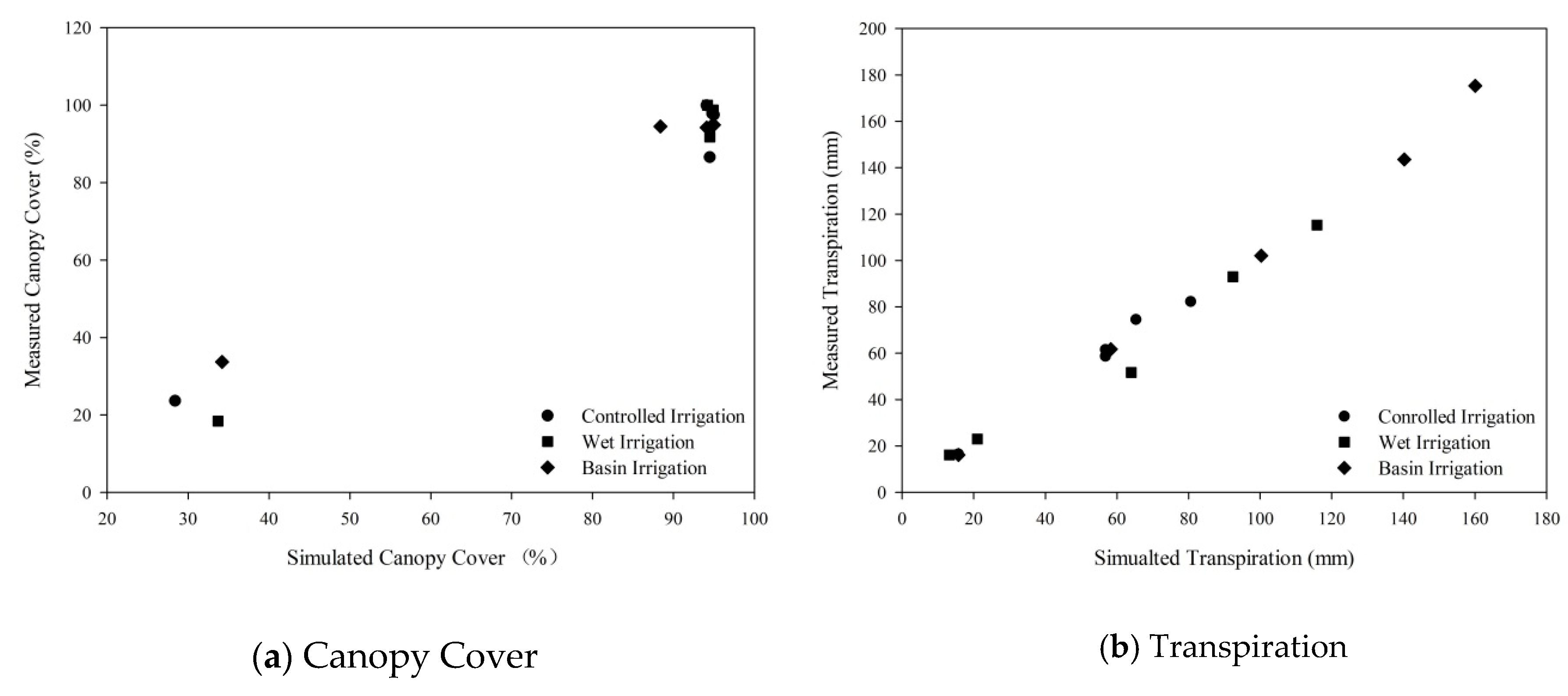
Since the irrigation scenarios set in this paper involve controlled irrigation, wet irrigation and basin irrigation methods, to improve the applicability of the AquaCrop model, the data for controlled irrigation during the whole growth period of rice (the regreening stage, tillering stage, jointing stage, heading stage and milky stage) in the field in 2010 were selected to calibrate the AquaCrop model. The simulated canopy cover, transpiration and yield were compared with the measured values, and the parameters were constantly adjusted until the measured values were infinitely close to the simulated values. Some of the parameters after calibration are shown in

Table 2. AquaCrop model rice main parameter list.

Model Parameter	Description	Recommended Value	Calibration Value
CGC	Canopy growth rate (%/growing degree day (GDD))	0.05–0.07	0.065
CDC	Canopy decay rate (%/GDD)	0.004	0.004
CCmax	Maximum canopy coverage (%)	80–99	99
Zx	Maximum effective root depth (m)	1.5	1.6
Kctr,x	Crop coefficient	1.1	1.2
HI0	Reference harvest index (%)	45–50	48
WP*	Normalized water production efficiency (g/m2)	15–20	19
CC0	Canopy coverage at 90% emergence (%)	1.5	1.5
Psen	Premature aging threshold (%)	0.85	0.76
Bredep	Respiratory depression point (%)	5	10
Stbio	The minimum daily growth degree of biomass accumulation without stress (°C/day)	13–15	20
Tteme	sowing to emergence (GDD)		13
Ttmrp	sowing to maximum rooting depth (GDD)		369
Ttsen	sowing to start of canopy senescence (GDD)		1153
Ttmat	sowing to maturity (GDD)		1167
Tflo	sowing to flowering (GDD)		836
	Length building up of HI (GDD)		283

.

The basic parameters remained unchanged after the rate was determined. The experimental data for field wet irrigation and basin irrigation during the full growth period of rice in 2010 were used to verify the accuracy of the model. The simulation results for canopy cover and transpiration are shown in Figure 3. However, the simulated production values for controlled, wet and basin irrigation were all less than the measured values, which were 13.70%, 7% and 7.79%, respectively.

In this paper, the normalized root mean square error (NRMSE), Nash efficiency coefficient (NSE) and determination coefficient R² [36] are selected to evaluate the degree of coincidence between the simulated and measured values of the model [37]. The model validation results are shown in

Table 3. Calibrated crop parameters.

Treatment	Canopy Cover			Transpiration			Yield
	NRMSE (%)	NSE	R2	NRMSE (%)	NSE	R2	NRMSE (%)	NSE	R2
Controlled Irrigation	6.410	0.968	0.974	8.110	0.956	0.984	9.495	0.793	0.993
Wet Irrigation	9.522	0.940	0.992	9.586	0.978	0.996
Basin Irrigation	9.303	0.941	0.997	7.185	0.984	0.981

. If NRMSE < 10%, the simulation value is considered excellent; if NRMSE is greater than 10% but less than 20%, the simulation value is considered good; when 20% < NRMSE < 30%, the simulation value is considered bad. The NSE is a relative error index, which is a dimensionless model evaluation index. When the value is close to 1, the model is highly reliable; when the value is close to 0, the simulation results are generally reliable, but the simulation process error is large. The value of the determination coefficient reflects the degree of correlation. The closer R² is to 1, the higher the reference value of the related equation is; conversely, the closer R² gets to 0, the lower the reference value is. The model validation results are shown in Table 3. The specific index evaluation equations of the model are as follows:

$$\mathrm{NRMSE}=\frac{100}{{\mathrm{O}}_{\mathrm{ave}}}\sqrt{\frac{1}{\mathrm{N}}{\displaystyle \sum }_{\mathrm{i}=1}^{\mathrm{N}}{\left({\mathrm{O}}_{\mathrm{i}}-{\mathrm{S}}_{\mathrm{i}}\right)}^2}$$

(7)

$$\mathrm{NSE}=1-\frac{{{\displaystyle \sum }}_{\mathrm{i}=1}^{\mathrm{N}}{\left({\mathrm{O}}_{\mathrm{i}}-{\mathrm{S}}_{\mathrm{i}}\right)}^2}{{{\displaystyle \sum }}_{\mathrm{i}=1}^{\mathrm{N}}{\left({\mathrm{O}}_{\mathrm{i}}-{\mathrm{O}}_{\mathrm{ave}}\right)}^2}$$

(8)

$${\mathrm{R}}^2=\frac{{\left[{{\displaystyle \sum }}_{\mathrm{i}=1}^{\mathrm{N}}\left({\mathrm{O}}_{\mathrm{i}}-{\mathrm{O}}_{\mathrm{ave}}\right)\left({\mathrm{S}}_{\mathrm{i}}-{\mathrm{S}}_{\mathrm{ave}}\right)\right]}^2}{{{\displaystyle \sum }}_{\mathrm{i}=1}^{\mathrm{N}}{\left({\mathrm{O}}_{\mathrm{i}}-{\mathrm{O}}_{\mathrm{ave}}\right)}^2{{\displaystyle \sum }}_{\mathrm{i}=1}^{\mathrm{N}}{\left({\mathrm{S}}_{\mathrm{i}}-{\mathrm{S}}_{\mathrm{ave}}\right)}^2}$$

(9)

where O_i (i = 1, 2, …, N) is the measured value, S_i (i = 1, 2, …, N) is the analog value, O_ave is the average of all observed values, S_ave is the average of all simulated values, and N is the number of data.

As shown in Table 3, the NRMSE values of the canopy cover, yield and transpiration are less than 10%, which indicates that the simulation values are excellent. The simulation precision for canopy cover is higher than those for transpiration and yield. The NSE values of transpiration were all above 0.9 and close to 1, indicating high reliability. The R² of the yield was 0.993, which is close to 1, indicating a high reference value for calibration. The results show that the AquaCrop model has an excellent simulation effect, which verifies that the model can be used to simulate rice growth.

3.2. Analysis of the Rice Irrigation Schedule Simulation Results Under the Different Scenarios

According to preliminary experiments and simulations, when the FC reaches 30% or above, the changes in irrigation water amount, irrigation times and FC have little impact on the yield. Therefore, the analysis is carried out when the FC is 20%, 25% and 30%.

3.2.1. Effect of the Irrigation Amount on the Rice Yield during the Growth Period

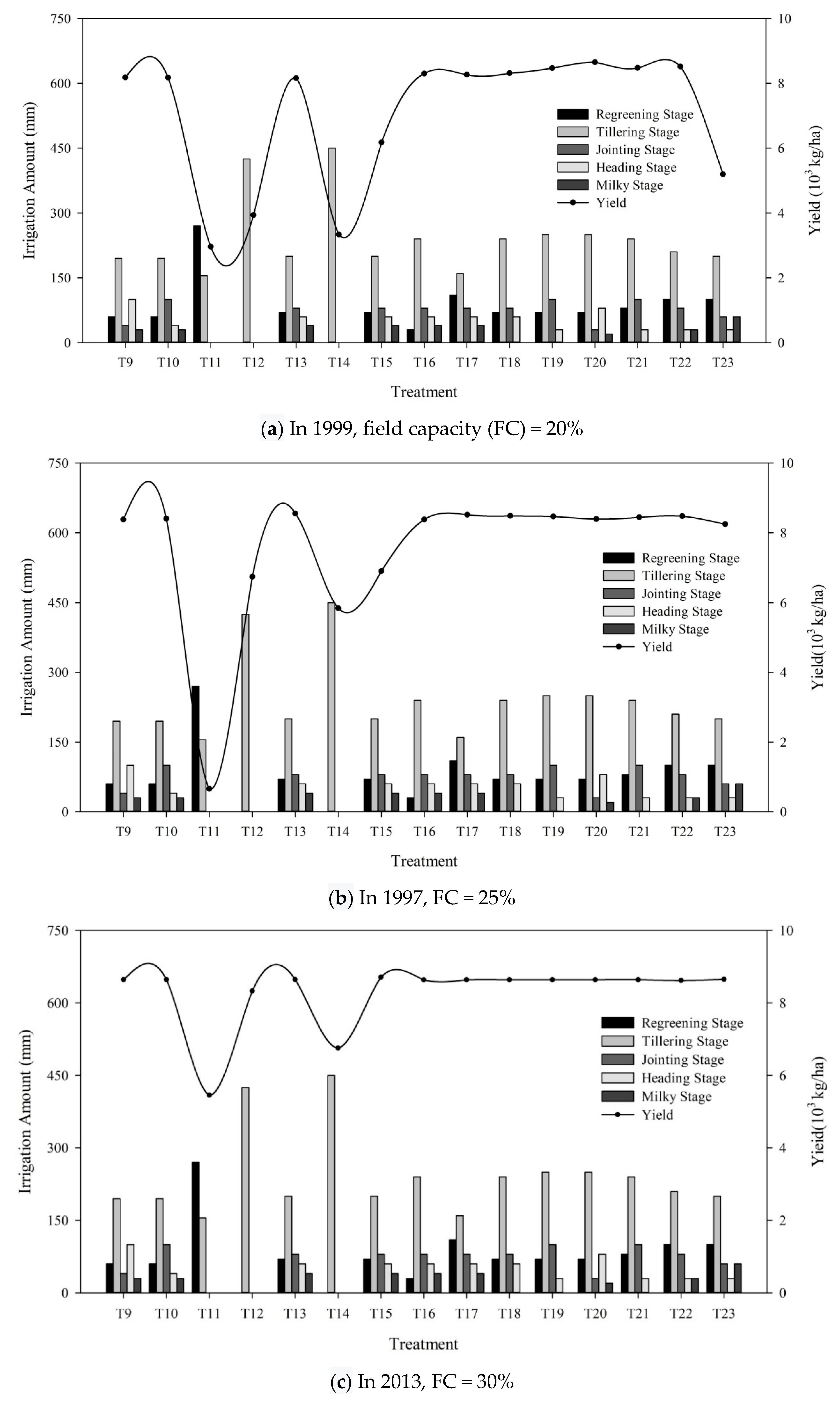
The irrigation scenarios described in Section 2.3.1 are input into the calibrated AquaCrop model, and then the relationship between the water yield of rice in the different irrigation scenarios of the three rainfall years and the irrigation water amount in each growth period is obtained (Figure 3).

In the figure, T1–T28 represent the settings of 28 irrigation scenarios. At this time, when only considering the influences of the same irrigation water amount and the water allocation in each growth period on the yield, the T9–T23 treatments were selected for discussion. According to Figure 4, when the other factors are the same, the yield increases with increasing irrigation amount. When the irrigation was concentrated at the tillering stage, the irrigation water quantity increased and the yield increased. Daily irrigation of the same amount at the beginning of the regreening stage would reduce the yield, such as treatment T11; daily equivalent irrigation at the tillering stage, continuous irrigation of 30 mm every day or equal irrigation every other day (each irrigation is 40 mm) would also reduce the yield, such as treatments T12 and T14, resulting in a rice yield reduction of 4.5 × 10³–5.3 × 10³ kg/ha. When no intensive irrigation occurred at the tillering stage, scattered irrigation increases the yield slightly, such as treatment T21. A small amount of irrigation at the milky stage can lead to a recovery in the yield, and the yield at the beginning of the regeneration period is lower than that at the end of the regeneration period, such as treatment T13 vs. treatment T18. When the amount of irrigation water at the regreening stage is too large, such as treatment T17, 110 mm of irrigation at the regreening stage reduces the yield.

It is not necessary to consider the rainfall during the regreening stage, and only a small amount of irrigation can be carried out during the growth period to obtain a higher rice yield. Therefore, to improve the rice yield, a small amount of irrigation should be carried out at the regreening stage. The total irrigation during the growth period is 50–70 mm, but irrigation should not be carried out at the early regreening stage. Irrigation was concentrated at the tillering stage, which allocated more water compared to the other growing stages, even more than the total irrigation at the other growing stages. Irrigation should be conducted according to the rainfall between the jointing stage, heading stage and milky stage, and less irrigation should occur when rainfall is high, while more irrigation should be conducted when rainfall is low.

3.2.2. Effect of the Total Irrigation Amount on the Crop Yield

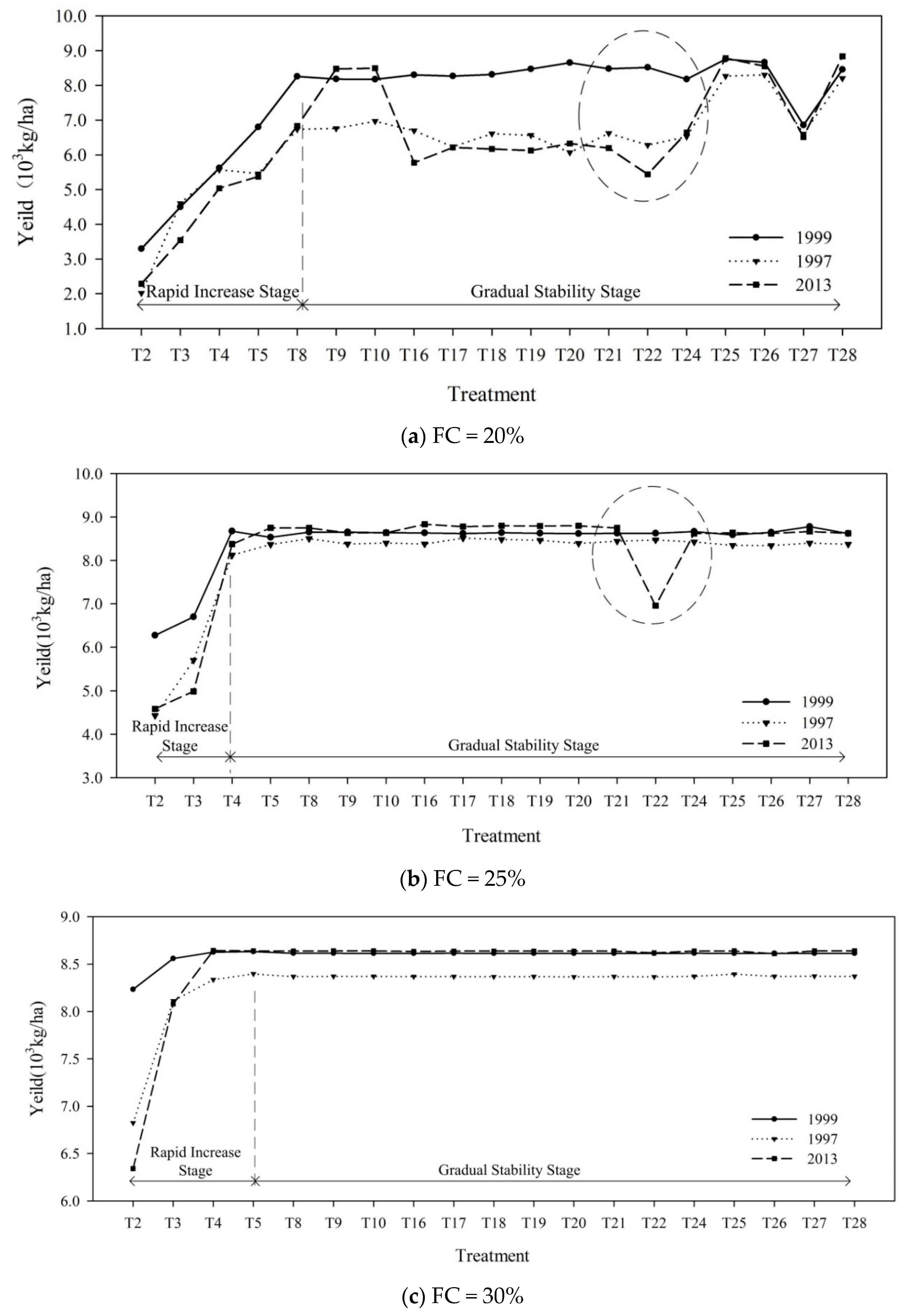
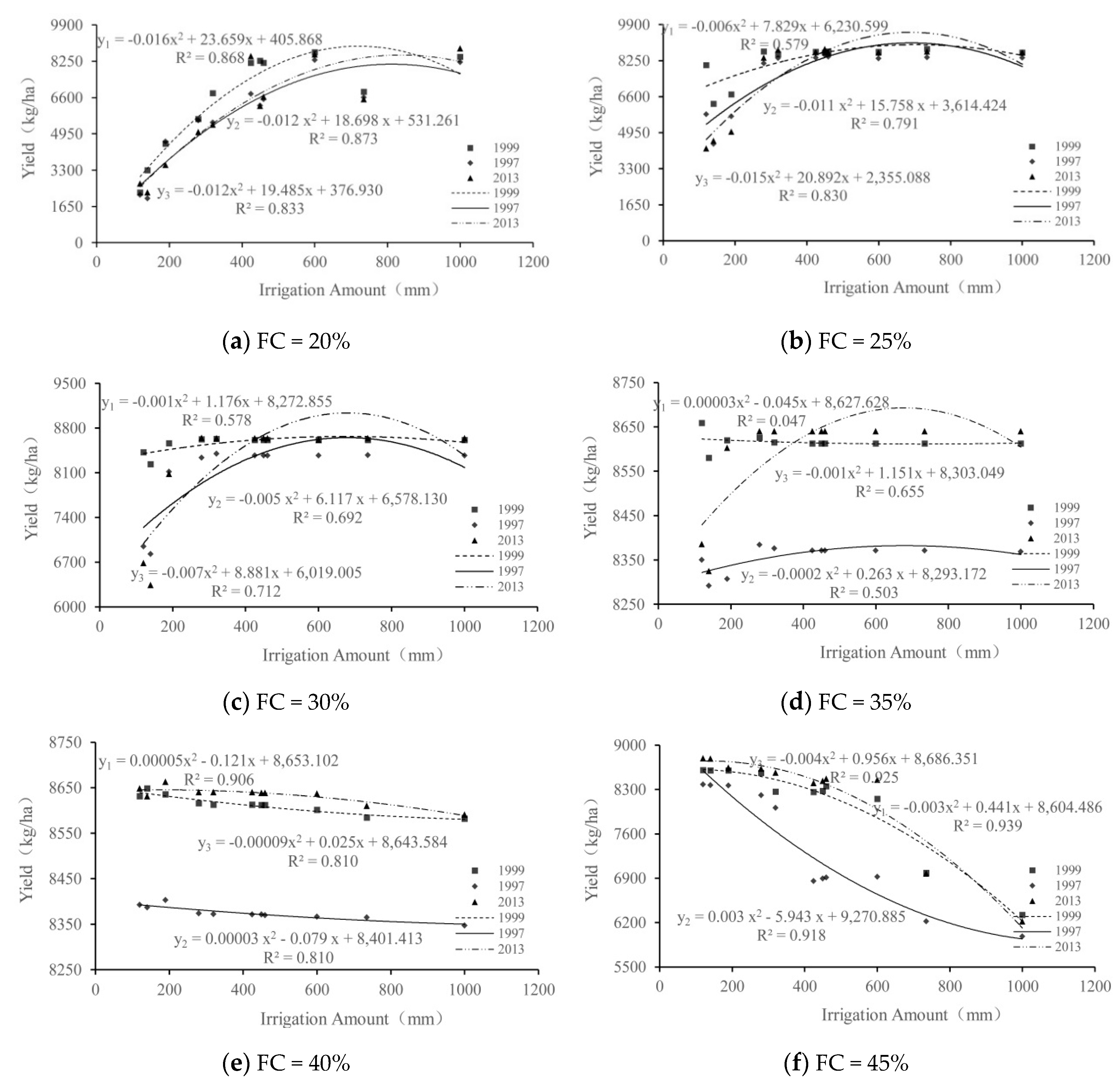
The relationship between the irrigation quota and yield under the different treatment conditions is shown in Figure 5.

Since the yield of rice under the T1 treatment was too low, the T1 data were omitted for the sake of simplification. As shown in Figure 5, the change in rice yield with the irrigation quota can be divided into two stages: one stage is the rapid increase stage, in which the rice yield increases rapidly with the increase in irrigation quota; and the second stage is the gradual stability stage. When the irrigation quota reaches a certain amount of water, the irrigation continues to increase, and the rice yield does not increase significantly but remains at a higher level or fluctuates slightly. The rice yield at the different FC has the same trend as the overall change in irrigation water amount, which can be divided into two stages, the rapid growth and gradual stability stages, and how quickly rice enters the stable stage is accelerated with the increase in FC. When the FC is 20%, the rice yield at the stable stage fluctuates greatly. Figure 5a shows that the rice yield at the stable stage shows a low-yield period in the wet year, indicating that when the rainfall is high, the irrigation water in a certain growth period will reduce the rice yield. Figure 5a,b show a drop point (the circled parts in the figure), so it can be seen that different irrigation times will also have an impact on the yield when the irrigation amount is the same. When the FC increases, the influence of the irrigation amount on the rice yield weakens, and the rice yield does not fluctuate, as shown in Figure 5c.

In the dry year, for example, in 1999, in the rice growth period, the precipitation is low and the water deficit is serious. After 190 mm of supplementary irrigation, the yield could reach more than 4490 kg/ha, and irrigation has a great potential to increase the yield. For every 100 mm of supplementary irrigation at the growth stage, the yield increased by 1872 kg/ha, and for every 100 mm of supplementary irrigation at the stable stage, the yield increased by 270 kg/ha; the intensity of yield increase was significantly weakened. In the dry year, for example in 1997, the yield could reach more than 4600 kg/ha after 190 mm of supplementary irrigation. At the growth stage, the yield increased by approximately 1900 kg/ha for every 100 mm of supplementary irrigation. At the stable stage, the yield increased by 390 kg/ha for every 100 mm of supplementary irrigation, and the increase intensity was weakened. Supplementary irrigation of rice to reach the maximum yield level range requires 450 mm of water. In the dry year, for example, in 2013, the yield can reach more than 3540 kg/ha after 190 mm of supplementary irrigation. For every 100 mm of supplementary irrigation at the growth stage, the yield increases by approximately 1790 kg/ha; for every 100 mm of supplementary irrigation at the stable stage, the yield increases by approximately 490 kg/ha, and the increase in intensity of the yield decreases.

Based on the change trend of the yield with the irrigation quota, the relationship between the yield and irrigation quota was established through fitting. Figure 6 shows the fitted functional relations, where y₁, y₂ and y₃ are the fitted relations between the rice yield and irrigation water amount in 1999, 1997 and 2013, respectively.

In the three typical years, the quadratic function can more accurately describe the relationship between the total irrigation water amount and rice yield compared with a linear equation. The highest value of R² reaches 0.9, indicating that the fitting accuracy is excellent. When FC is between 20% and 35%, the fitting effect of the dry year is the weakest. When FC is 35%, the fitting effect of the quadratic function is not good. When FC is greater than 35%, the fitting precision is higher, but the coefficient of the quadratic term is small; hence, the data can be fitted by a linear relation, and the linear fitting effect is more accurate. According to the analysis in Figure 5, when the irrigation water amount is the same and FC is 20%, the yield in the dry years is higher than that in the normal years. When FC is between 25% and 45%, the yield in the wet years is higher than that in the dry years.

3.3. Rice Irrigation Schedule Optimization and Program Evaluation

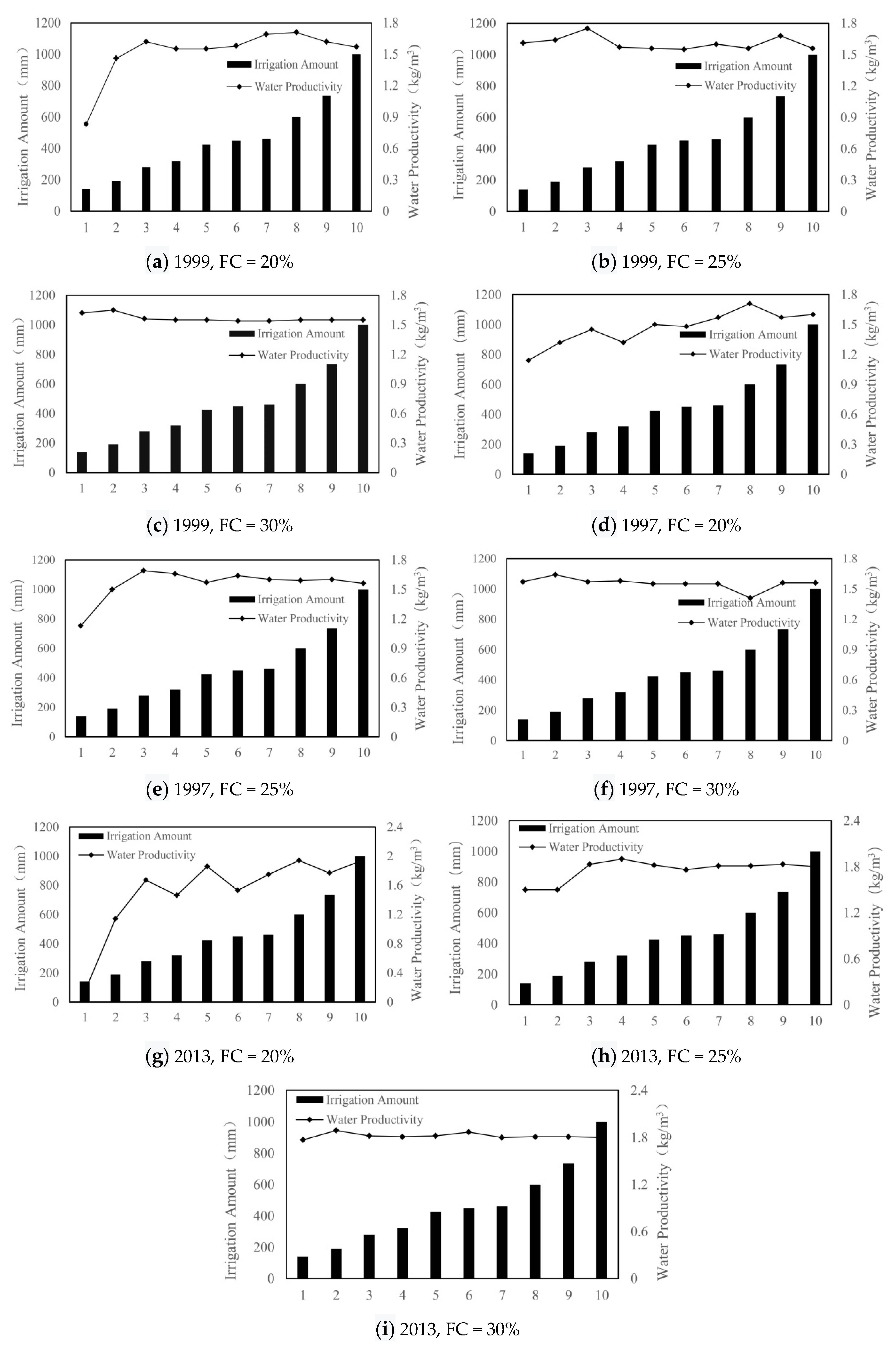
WP refers to the yield or output value obtained per unit of water resources under certain crop variety and cultivation conditions. Figure 7 shows the relationship between WP and irrigation water amount in the three typical years.

Figure 7 shows that WP changes with the irrigation water amount in three stages. The first stage is the increase stage, in which the WP of rice increases rapidly with the increase in irrigation quota. At this stage, the rate of WP increases faster than the rate of the irrigation amount. At this time, the irrigation water can be fully absorbed and utilized by plants; the second stage is the decline stage. When the irrigation quota reaches a certain amount of water, the irrigation water quantity will continue to increase, and WP will slightly decrease. At this time, the rice yield will increase or remain stable with increasing irrigation water amount, and the increase in yield is consistent with or lower than the increase in irrigation water amount; the third stage is the stable phase, which occurs when the irrigation amount is greater than 500 mm, and WP begins to slowly recover and gradually stabilizes; WP in the stable phase does not increase as the irrigation amount increases, and the growth rate of the yield is lower than the growth rate of the irrigation amount. Continued irrigation will not cause a surge in production, because the irrigation water cannot contribute positively to the rice yield. Therefore, the irrigation schedule of rice was optimized according to the growth of rice.

Through cloud model calculations based on the entropy method, the irrigation scenario with the maximum comprehensive evaluation value among the typical rainfall year simulation scenarios was obtained, and the optimal irrigation schedule of the different precipitation years based on cloud model optimization of multiple indicators was obtained.

Table 4. Optimal irrigation schedule for the different years.

Model Year	Comprehensive Evaluation Value	FC (%)	Treatment	Irrigation Quota (mm)	Irrigation Times	Yield (103 kg/ha)
Wet Year	8.3	25%	T10	425	17	8.637
	8.2	30%	T10	425	17	8.64
	8.1	40%	T12	425	17	8.64
	8.1	25%	T16	450	14	8.834
	8.1	25%	T17	450	14	8.781
Normal Year	8.1	25%	T20	450	14	8.392
	8.05	25%	T13	450	14	8.55
	8.05	25%	T17	450	14	8.516
	7.9	25%	T10	425	17	8.404
	7.8	25%	T5	320	16	8.368
Dry Year	7.98	25%	T10	425	17	8.64
	7.9	30%	T11	425	14	6.669
	7.8	25%	T15	450	11	8.76
	7.75	25%	T17	450	14	8.62
	7.75	35%	T11	425	14	8.123

shows the irrigation schemes with the top five comprehensive evaluation values in the three typical years.

There is abundant water in 2010, and the measured optimized irrigation amount in 2010 is 600 mm; the simulation model calculates a rice control irrigation quota of 460 mm in a wet year, which is 40% higher than 425 mm but 30% lower than the high yield treatment of irrigation water in 2010, but the simulation output is not lower than the trial production of 2010. This finding shows that the optimized irrigation schedule can not only ensure a high rice yield but can also realize water savings in the irrigation area.

4. Discussion

Most of the traditional irrigation schedule optimization methods take the maximum yield, minimum irrigation amount or maximum WP as optimization goals, and less consideration is given to field drainage optimization. However, irrigation schedule optimization can effectively reduce the displacement of paddy fields and reduce the emission of paddy fields. This paper considers the optimization of drainage irrigation schedules, which can effectively control the water and fertilizer losses and improve the utilization rate of irrigation water.

The use of a crop growth simulation model can greatly reduce the time and cost of the experiment and allow better design combinations, which is suitable for the simulation of more experimental scheme factors and levels. Pirmoradian [38] used the AquaCrop model to simulate the NRMSE of rice evapotranspiration in Iran, which was 18.45%. In this paper, the AquaCrop model was introduced into rice growth simulation in the Longtouqiao irrigation district of the Sanjiang Plain, China, and the simulated values were in good agreement with the measured values. The evapotranspiration NRMSE values in the three typical years reached 8.110%, 9.586% and 7.185%, thereby verifying that the model was highly applicable to rice growth simulation in this area.

Liu Guangming [39] used the Jensen model as a mathematical model for dynamic rice irrigation planning and calculated that the yield ratio was 0.8683 when the water-saving and efficient rice irrigation schedule prescribed 440 mm of irrigation during the whole growth period; when irrigation was 520 mm, the yield ratio was 0.9367. Fu Hong [40] analyzed the middle hybrid rice yield in the Longquanshan irrigation district by studying different irrigation methods and determined the optimal water-saving irrigation method for rice in the Longquanshan irrigation district. The results showed that the highest yield was 8542.5 kg/ha, followed by 8314.5 kg/ha, 7654.5 kg/ha and 6883.5 kg/ha. In this paper, selecting the yield, irrigation schedule, WP and displacement as indicators, the AquaCrop crop growth model and entropy-cloud model are combined to construct the optimal rice irrigation schedule model for the Longtouqiao irrigation district. Compared with Liu Guangming’s results, the irrigation amount during the whole growth period decreased by 100 mm, and the maximum yield of 9000 kg/ha decreased by 400 kg/ha. Compared with Fu Hong’s experiment, the rice yield increased by 30%. When studying the irrigation schedule, Shao Dongguo [41] introduced the factor of displacement. On this basis, the water allocation during each growth period and the optimal irrigation times of each growth period were considered. Compared with the previous rice irrigation schedule optimization studies with different growth periods, this study proposes a new method for crop irrigation schedule optimization.

The AquaCrop model cannot consider the effects of different varieties on the output variables, so in this paper the experimental data are based on a single rice variety. AquaCrop simulates herb crop responses to irrigation, and is especially useful when water is the key limiting factor for crop production. Therefore in this paper, we selected a variety of rice with a high demand for water.

5. Conclusions

In this study, rate determination and verification of the AquaCrop model were carried out by using data from rice irrigation tests in the Longtouqiao irrigation district, Baoqing County. A model was used to simulate the yield and displacement of different irrigation scenarios in three typical years. A cloud model based on the entropy method with multiple indexes was adopted to optimize the irrigation schedule. The main conclusions are as follows.

(1)

The applicability of the AquaCrop model in northeast China was verified. After calibration and verification of the AquaCrop model parameters, the NRMSE and R² values of the yield were 9.949% and 0.993, respectively, proving that the AquaCrop model has a high precision in northeast China, thus providing the basis for the next step of using this model for rice growth simulation to propose rice irrigation schedule optimization methods.

(2)

The rice yield increase potential of irrigation in different precipitation years was simulated. Irrigation has the greatest potential to increase the rice yield in dry years, which requires 600 mm of irrigation. The yield increases by approximately 1440 kg/ha for every 100 mm of supplementary irrigation on average. In normal years, rice requires an irrigation amount of approximately 450 mm to reach the maximum yield level, and the yield can be increased approximately 1892 kg/ha for every 100 mm of supplementary irrigation. In wet years, approximately 450 mm of supplementary irrigation is required to reach the maximum rice yield range, and the yield can be increased by approximately 2032 kg/ha for every 100 mm of supplementary irrigation.

(3)

To maximize the yield, abundant irrigation should be carried out at the tillering stage, while little irrigation should be carried out at the regreening stage. During the rest of the rice growth period, irrigation should be carried out according to the growth period rainfall. When the rainfall in the growth period is high, irrigation should be carried out to a lesser degree, and when the rainfall is low, irrigation should be increased.

(4)

The optimal irrigation schedule was as follows: in dry years, at an FC of 25%, the total irrigation water amount is 425 mm, and irrigation should be conducted 17 times; in normal years, at an FC of 25%, the total irrigation water amount is 450 mm, and irrigation should be conducted 14 times; in wet years, at an FC of 25%, the total irrigation water amount is 425 mm, and irrigation should be conducted 17 times.

References

- Zhang, C.; Chen, X.X.; Li, Y.; Ding, W.; Fu, G.T. Water-energy-food nexus: Concepts, questions and methodologies. J. Clean. Prod. 2018, 195, 625–639. [Google Scholar] [CrossRef]
- Bouman BA, M.; Humphreys, E.; Tuong, T.P.; Barker, R. Rice and water. Adv. Agron. 2007, 92, 187–237. [Google Scholar]
- Cui, Z.L.; Zhang, H.Y.; Chen, X.; Zhang, C.; Ma, W.; Huang, C.; Zhang, W.; Mi, G.; Miao, Y.; Li, X.; et al. Pursuing sustainable productivity with millions of smallholder farmers. Nature 2018, 555, 363–366. [Google Scholar] [CrossRef] [PubMed]
- Yao, F.; Huang, J.; Cui, K.; Nie, L.; Xiang, J.; Liu, X.; Wu, W.; Chen, M.; Peng, S. Agronomic performance of high-yielding rice variety grown under alternate wetting and drying irrigation. Field Crops Res. 2012, 126, 16–22. [Google Scholar] [CrossRef]
- Fu, Q.; Li, L.; Li, M.; Li, T.; Liu, D.; Hou, R.; Zhou, Z. An interval parameter conditional value-at-risk two-stage stochastic programming model for sustainable regional water allocation under different representative concentration pathways scenarios. J. Hydrol. 2018, 564, 115–124. [Google Scholar] [CrossRef]
- Zhang, C.; Li, Y.; Chu, J.; Fu, G.; Tang, R.; Qi, W. Use of many-objective visual analytics to analyze water supply objective trade-offs with water transfer. J. Water Resour. Plann. Manag. 2017, 143, 05017006. [Google Scholar] [CrossRef]
- Zhang, R.P.; Ma, J.; Wang, H.Z.; Li, Y.; Li, X.Y. Effects of different irrigation methods on growth and development characteristics and water use efficiency in paddy rice. Chin. Agric. Sci. Bull. 2005, 21, 144–150. [Google Scholar]
- Hall, W.A.; Butcher, W.S. Optimal timing of irrigation. J. Irrig. Drain. Div. 1968, 94, 267–278. [Google Scholar]
- Dudley, N.J.; Howell, D.T.; Musgrave, W.F. Optimal intraseasonal irrigation water allocation. Water Resour. Res. 1968, 7, 770–788. [Google Scholar] [CrossRef]
- Lorber, A.; Wangen, L.E.; Kowalski, B.R. A theoretical foundation for the PLS algorithm. J. Chemom. 1987, 1, 19–31. [Google Scholar] [CrossRef]
- Sun, J.S.; Kang, S.Z.; Zhang, J.Y.; Hao, J.; Duan, A.W.; Yu, X.G.; Xiao, J.F. Schedules of irrigation for the high-yield and water-saving cultivation of winter wheat and summer maize in Huoquan irrigation district of Shanxi province. Trans. Chin. Soc. Agric. Eng. 2000, 16, 50–53. [Google Scholar]
- Cui, Y.L.; Li, Y.H.; Mao, Z. The optimal allocation of irrigation water with diversified crops under limited water supply. J. Hydraul. Eng. 1997, 3, 37–42. [Google Scholar]
- Fu, Q.; Wang, L.K.; Men, B.H.; Jin, J.L. A new method of optimizing irrigation system under non-sufficient irrigation—Multi-dimensional dynamic planning based on RAGA. J. Hydraul. Eng. 2003, 1, 123–128. [Google Scholar]
- Tian, F.Q.; Hu, H.P.; Yang, S.X. Computer simulation of irrigation water requirement for paddy rice. Trans. Chin. Soc. Agric. Eng. 1999, 15, 100–103. [Google Scholar]
- Yu, Z.J.; Shang, S.H. Multi-objective optimization method for irrigation scheduling of crop rotation system and its application in North China. J. Hydraul. Eng. 2016, 47, 1188–1196. [Google Scholar]
- Osama, S.; Elkholy, M.; Kansoh, R.M. Optimization of the cropping pattern in Egypt. Alex. Eng. J. 2017, 56, 557–566. [Google Scholar] [CrossRef]
- Dang, T.; Pedroso, R.; Laux, P.; Kunstmann, H. Development of an integrated hydrological-irrigation optimization modeling system for a typical rice irrigation scheme in Central Vietnam. Agric. Water Manag. 2018, 208, 193–203. [Google Scholar] [CrossRef]
- Li, M.; Fu, Q.; Singh, V.P.; Ji, Y.; Liu, D.; Zhang, C.; Li, T. An optimal modelling approach for managing agricultural water-energy-food nexus under uncertainty. Sci. Total Environ. 2019, 651, 1416–1434. [Google Scholar] [CrossRef]
- Li, M.; Fu, Q.; Singh, V.P.; Liu, D. An interval multi-objective programming model for irrigation water allocation under uncertainty. Agric. Water Manag. 2018, 196, 24–36. [Google Scholar] [CrossRef]
- Liu, X.; Guo, P.; Li, F.; Zheng, W. Optimization of planning structure in irrigated district considering water footprint under uncertainty. J. Clean. Prod. 2019, 210, 1270–1280. [Google Scholar] [CrossRef]
- Geerts, S.; Raes, D.; Garcia, M.; Taboada, C.; Miranda, R.; Cusicanqui, J.; Mhizha, T.; Vacher, J. Modeling the potential for closing quinoa yield gaps under varying water availability in the Bolivian Altiplano. Agric. Water Manag. 2009, 96, 1652–1658. [Google Scholar] [CrossRef]
- Dubey, S.K.; Sharma, D. Assessment of climate change impact on yield of major crops in the Banas River Basin, India. Sci. Total Environ. 2018, 635, 10–19. [Google Scholar] [CrossRef] [PubMed]
- Zhang, W.; Liu, W.; Xue, Q.; Chen, J.; Han, X. Evaluation of the AquaCrop model for simulating yield response of winter wheat to water on the southern Loess Plateau of China. Water Sci.Technol. 2013, 68, 821. [Google Scholar] [CrossRef] [PubMed]
- Evett, S.R.; Tolk, J.A. Introduction: Can water use efficiency be modeled well enough to impact crop management. Agron. J. 2009, 101, 423–425. [Google Scholar] [CrossRef]
- Jin, X.L.; Feng, H.K.; Zhu, X.K.; Li, Z.H.; Song, S.N.; Song, X.Y.; Yang, G.; Xu, X.; Guo, W. Assessment of the AquaCrop model for use in simulation of irrigated winter wheat canopy cover, biomass, and grain yield in the North China plain. PLoS ONE 2014, 9, e86938. [Google Scholar] [CrossRef] [PubMed]
- Ni, L.; Feng, H.; Ren, X.C.; Hao, Z.P. Applicable evaluation of crop model AquaCrop for summer maize production in Loess Plateau region. Agric. Res. Arid Areas 2015, 33, 40–45. [Google Scholar]
- Sun, A.H. Study on Water-Fertilizer Effect and Irrigation Models of Rice in Sanjiang Plain. Ph.D. Thesis, Northeast Agricultural University, Harbin, China, 2011. [Google Scholar]
- Boudhina, N.; Masmoudi, M.M.; Alaya, I.; Jacob, F.; Mechlia, N.B. Use of AquaCrop model for estimating crop evapotranspiration and biomass production in hilly topography. Arab. J. Geosci. 2019, 12, 259. [Google Scholar] [CrossRef]
- Seyed, R.R.; Soufizadeh, S.; Amiri Larijani, B.; AghaAlikhani, M.; Kambouzia, J. Simulation of growth and yield of various irrigated rice (Oryza sativa L.) genotypes by AquaCrop under different seedling ages. Nat. Resour. Model. 2018, 31, e12162. [Google Scholar] [CrossRef]
- Manivasagam, V.S.; Nagarajan, R. Rainfall and crop modeling-based water stress assessment for rainfed maize cultivation in peninsular India. Theor. Appl. Climatol. 2018, 132, 529–542. [Google Scholar] [CrossRef]
- Cai, Q.K.; Li, E.J.; Tao, L.L.; Jiang, R.B. Farmland soil moisture retrieval using PROSAIL and water cloud model. Trans. Chinese Soc. Agric. Eng. 2018, 34, 117–123. [Google Scholar]
- Li, J.; Fang, H.; Song, W.Y. Sustainable supplier selection based on SSCM practices: A rough cloud TOPSIS approach. J. Clean. Prod. 2019, 222, 606–621. [Google Scholar] [CrossRef]
- Cheng, K.; Fu, Q.; Ren, Y.T.; Guo, J.; Lu, X.P. Evaluation of bearing capacity of water resources in Heilongjiang province based on entropy weight and cloud model. J. Northeast Agric. Univ. 2015, 46, 75–80. [Google Scholar]
- Hu, Y.L.; Chen, Z.G.; Liu, Z.G. Study of the utilization efficiency of water resources in Hebei province based on the entropy method. Chin. J. Agric. Res. Reg. Plan. 2015, 36, 136–142. [Google Scholar]
- Mrabet, E.; Guedri, M.; Ichchou, M.N.; Ghanmi, S.; Soula, M. A new reliability based optimization of tuned mass damper parameters using energy approach. J. Vib. Control 2018, 24, 153–170. [Google Scholar] [CrossRef]
- Das, B.; Nair, B.; Reddy, V.K.; Venkatesh, P. Evaluation of multiple linear, neural network and penalised regression models for prediction of rice yield based on weather parameters for west coast of India. Int. J. Biometeorol. 2018, 62, 109–1822. [Google Scholar] [CrossRef] [PubMed]
- Song, J.; Li, J.; Yang, Q.H.; Mao, X.M.; Yang, J.; Wang, K. Multi-objective optimization and its application on irrigation scheduling based on AquaCrop and NSGA-II. J. Hydraul. Eng. 2018, 49, 1284–1295. [Google Scholar]
- Pirmoradian, N.; Davatgar, N. Simulating the effects of climatic fluctuations on rice irrigation water requirement using AquaCrop. Agric. Water Manag. 2019, 213, 97–106. [Google Scholar] [CrossRef]
- Guangming, L.; Jinsong, Y.; Yan, J.; Xiuyong, Z. Optimized rice irrigation schedule based on controlling irrigation theory. Trans. Chin. Soc. Agric. Eng. 2005, 21, 29–33. [Google Scholar]
- Fu, H. Effects of Different Water-Saving Irrigation Methods on Form of Medium Hybrid Rice Production in Longquan Mountain Irrigation Area. Ph.D. Thesis, Sichuan Agricultural University, Chengdu, China, 2013. [Google Scholar]
- Shao, D.G.; Le, Z.H.; Xu, B.L.; Hu, N.J.; Tian, Y.N. Optimization of irrigation scheduling for organic rice based on AquaCrop. Trans. Chin. Soc. Agric. Eng. 2018, 34, 114–122. [Google Scholar]
Figure 1.
Study area.
Figure 2.
Study process.
Figure 3.
Model simulation result.
Figure 4.
Relationship diagram of the irrigation amount and yield during the growth period.
Figure 5.
Diagram of the relationship between the irrigation quota and yield under the different treatment conditions.
Figure 6.
The fitting diagram of the irrigation water quantity and yield.
Figure 7.
Water productivity (WP) map.