Combining Soil Erosion Modeling with Connectivity Analyses to Assess Lateral Fine Sediment Input into Agricultural Streams


 and
and
Abstract
:1. Introduction
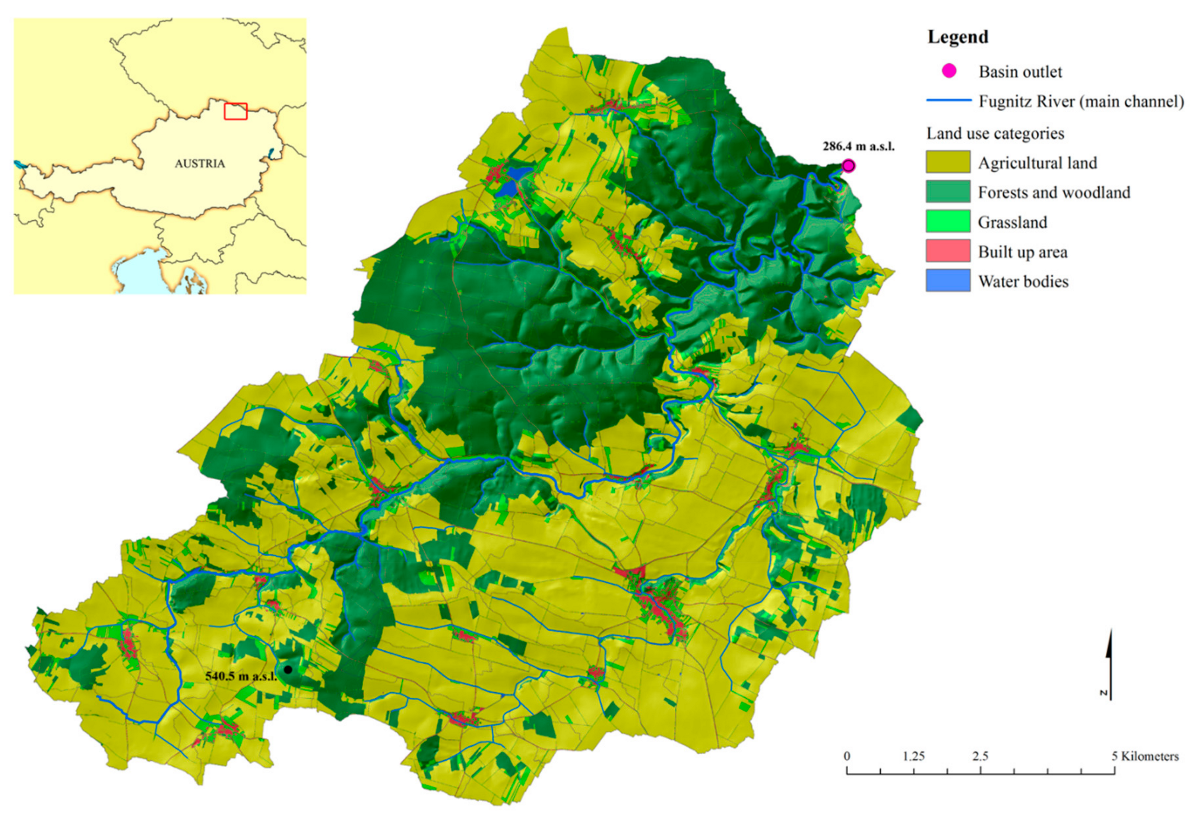
2. Study Area
3. Methods
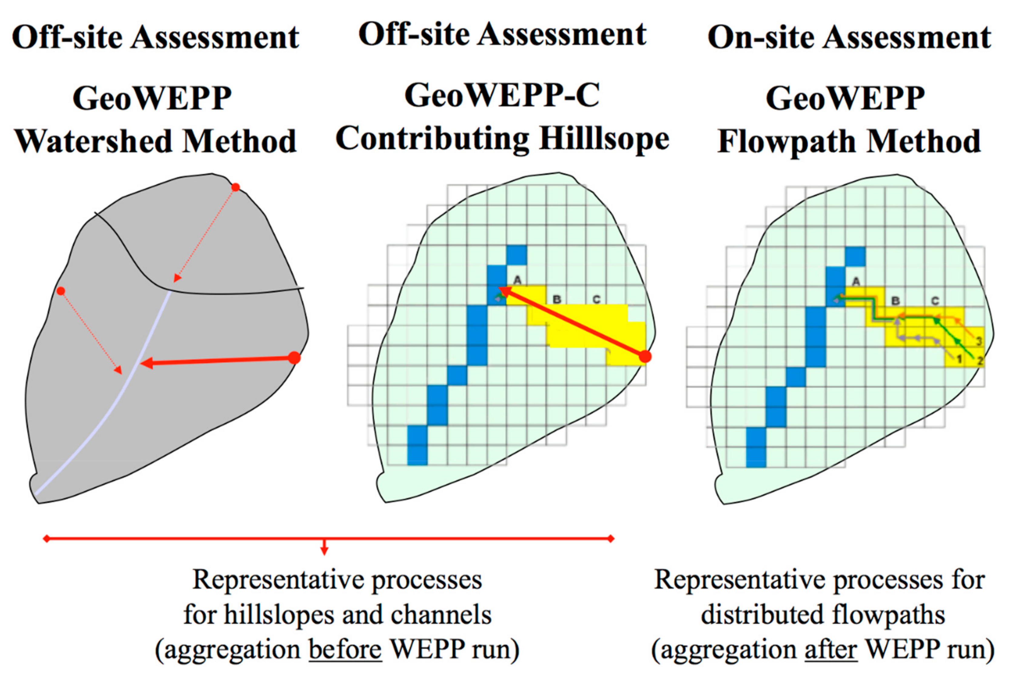
3.1. Soil Erosion Modeling (GeoWEPP)
3.2. Index of Connectivity (IC) Calculations
3.3. Connectivity Mapping in the Field
3.4. Incorporating Connectivity into GeoWEPP: GeoWEPP-C
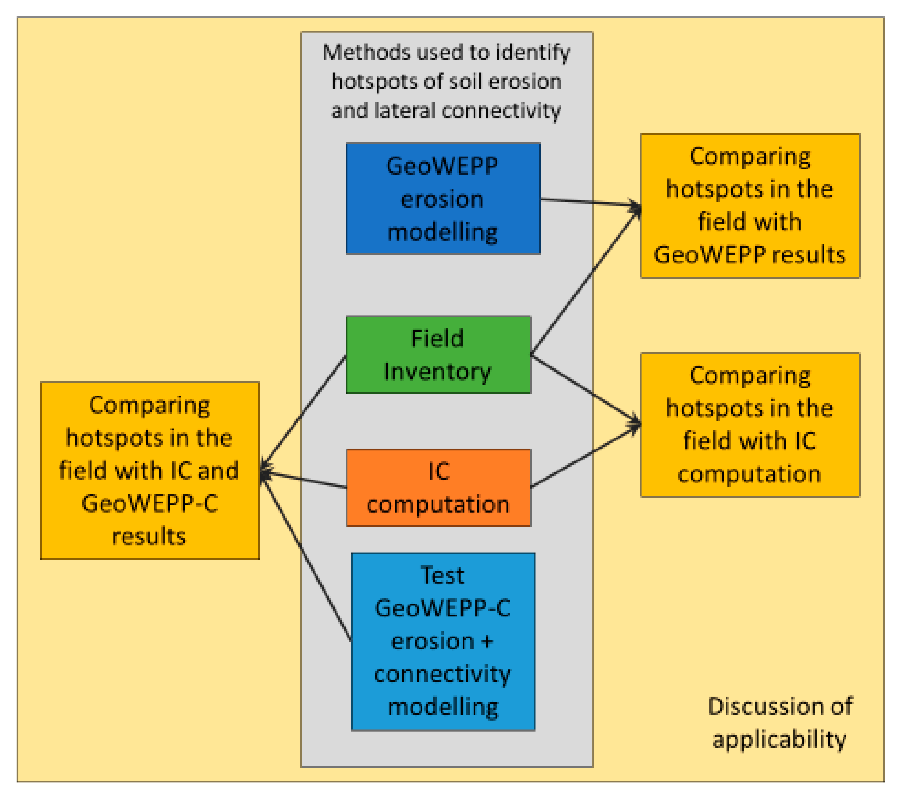
3.5. Inter-Comparison of Methods
4. Results
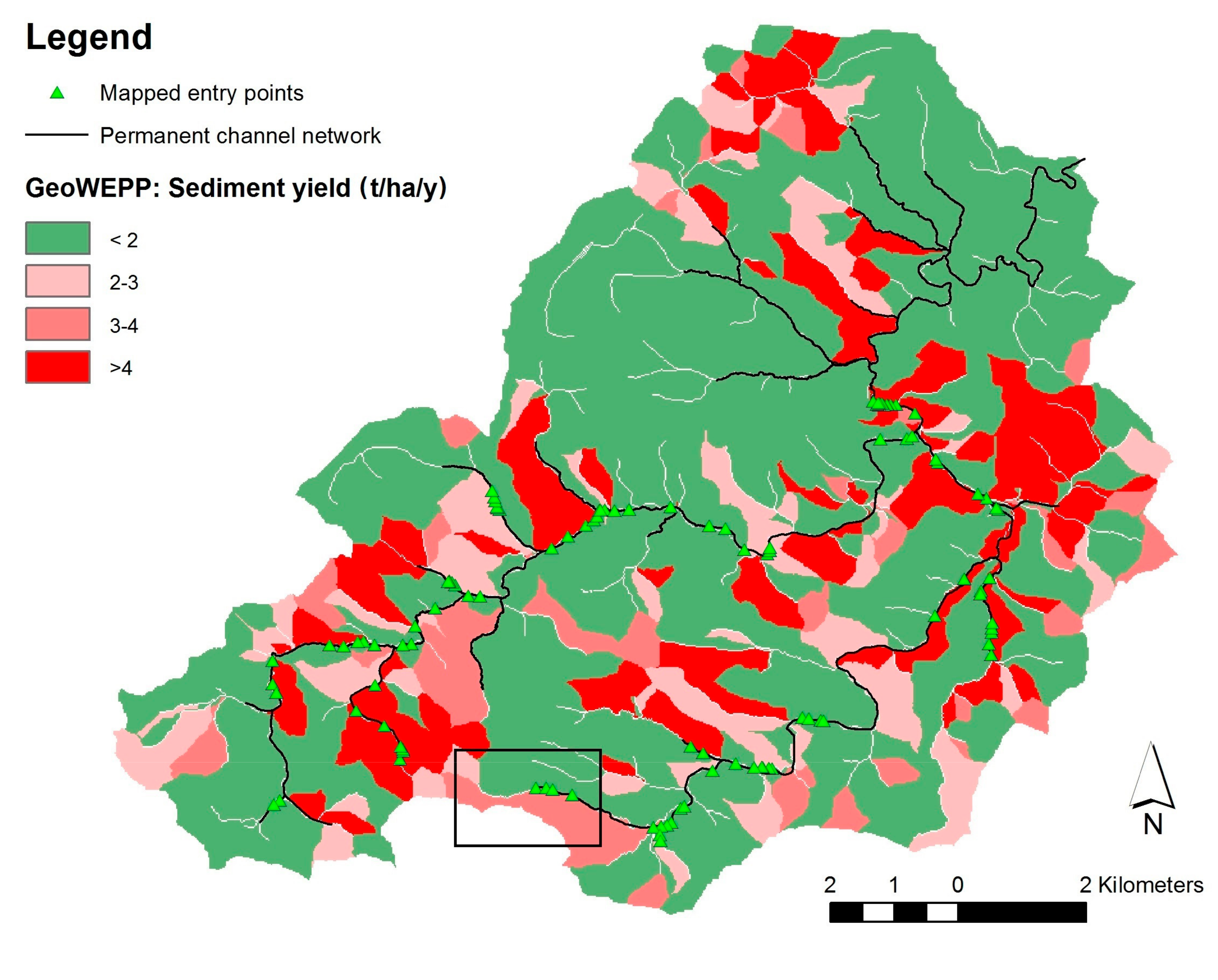
4.1. Soil Erosion Modeling (GeoWEPP)
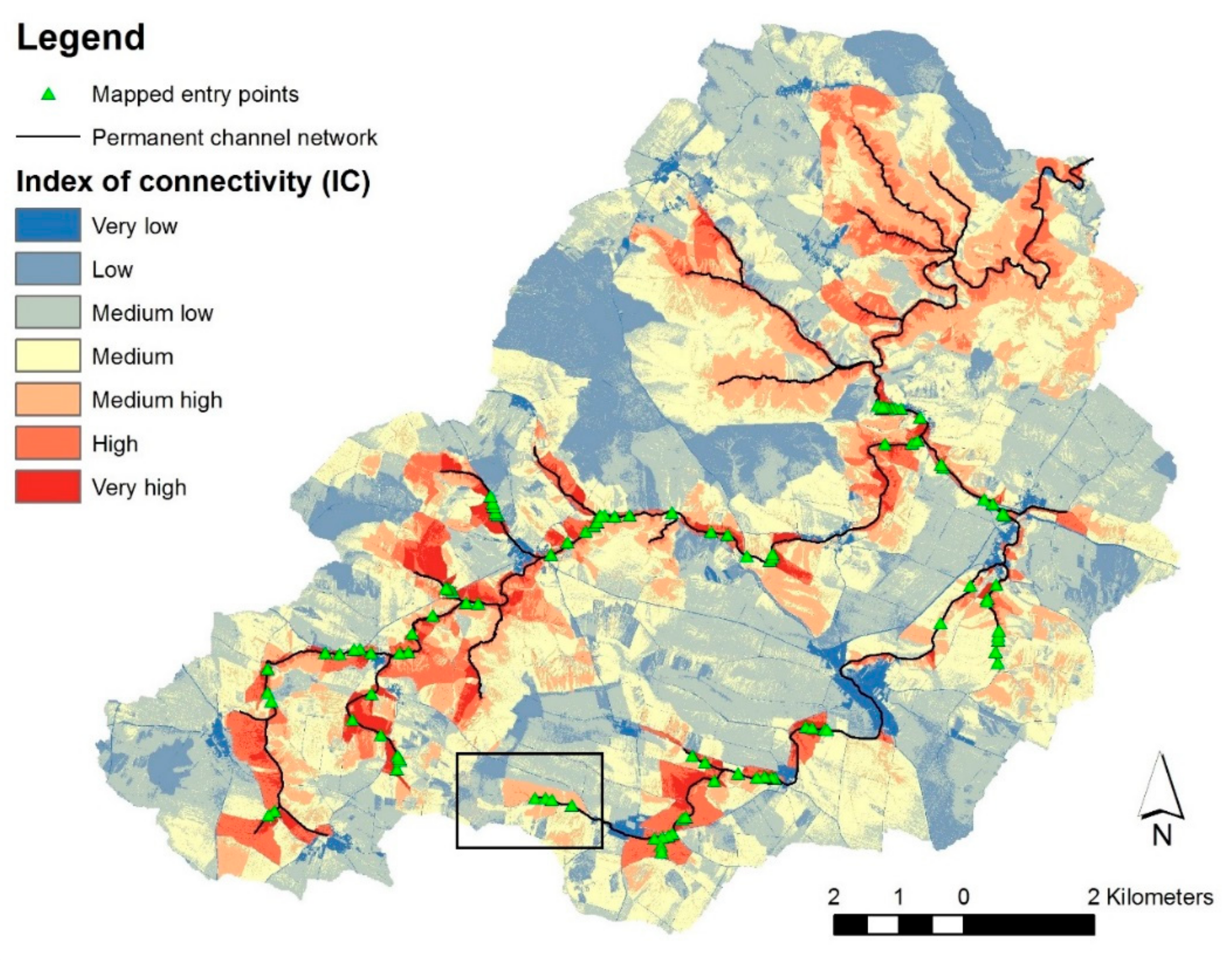
4.2. Index of Connectivity (IC) Calculations.
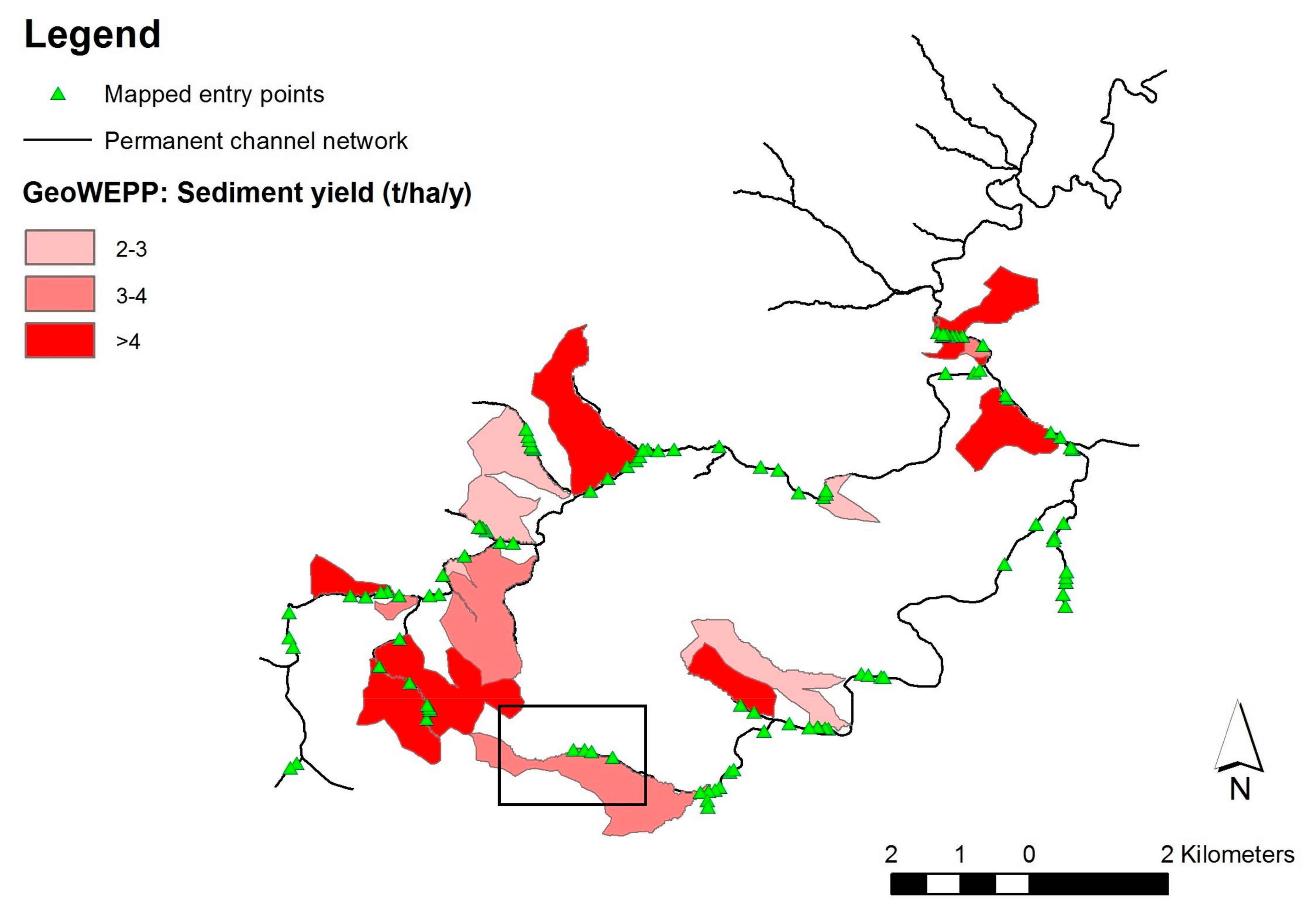
4.3. Connectivity Mapping, IC Validation, and Hot-Spot Delineation
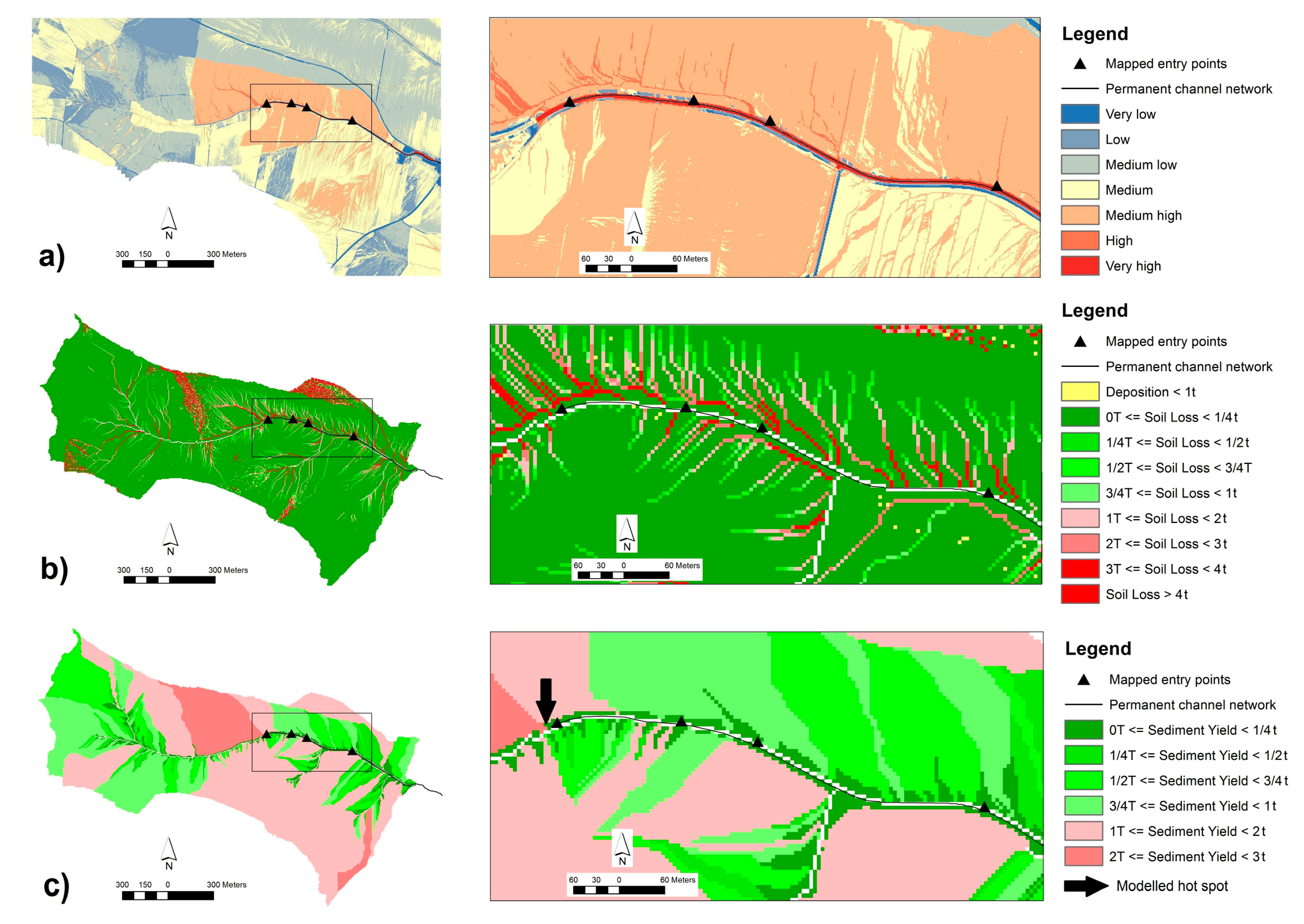
4.4. GeoWEPP-C Results for the Test Area
5. Discussion
5.1. Soil Erosion Modeling (GeoWEPP)
5.2. Index of Connectivity (IC)
5.3. GeoWEPP-C
6. Conclusions
- GeoWEPP is able to detect sub-catchments with high amount of soil erosion/sediment yield that represent manageable units in the context of soil erosion research and catchment management;
- Combining GeoWEPP modeling with field-based connectivity mapping has shown to be suitable for the delineation of lateral fine sediment connectivity hotspots;
- The IC is a useful tool for a quick GIS-based assessment of structural connectivity, however showing significant limitations for agricultural catchments which are mainly related (but not limited) to lacking information on functional aspects of connectivity;
- The process-based GeoWEPP-C model can be seen a methodical improvement when it comes to assess lateral sediment connectivity in agricultural catchments. However, the model needs some more improvement, especially for the high computational demanding use of the ever-increasing higher spatial resolution before it is ready for practical application (e.g., in the contexts of soil erosion and surface water management).
Author Contributions
Funding
Acknowledgments
Conflicts of Interest
References
- Graves, A.; Morris, J.; Deeks, L.; Rickson, J.; Kibblewhite, M.; Harris, J.; Farewell, T. The Total Costs of Soils Degradation in England and Wales. Ecol. Econ. 2015, 119, 399–413. [Google Scholar] [CrossRef]
- Lal, R. Soil erosion by wind and water: Problems and prospects. In Soil Erosion Research Methods; Routledge: New York, NY, USA, 1994; pp. 1–10. [Google Scholar]
- Pimentel, D. Soil erosion: A food and environmental threat. Environ. Dev. Sustain. 2006, 8, 119–137. [Google Scholar] [CrossRef]
- Glendell, M.; Brazier, R. Accelerated export of sediment and carbon from a landscape under intensive agriculture. Sci. Total Environ. 2014, 476, 643–656. [Google Scholar] [CrossRef] [PubMed]
- Pimentel, D.; Harvey, C.; Resosudarmo, P.; Sinclair, K.; Kurz, D.; McNair, M.; Crist, S.; Shpritz, L.; Fitton, L.; Saffouri, R.; et al. Environmental and economic costs of soil erosion and conservation benefits. Sci.-Aaas-Wkly. Pap. Ed. 1995, 267, 1117–1122. [Google Scholar] [CrossRef] [PubMed]
- Wardle, D.A.; Bardgett, R.D.; Klironomos, J.N.; Setala, H.; Putten, W.H.; Wall, D.H. Ecological linkages between aboveground and belowground biota. Science 2004, 304, 1629–1633. [Google Scholar] [CrossRef] [PubMed]
- Lal, R. Soil conservation and ecosystem services. Int. Soil Water Conserv. Res. 2014, 2, 36–47. [Google Scholar] [CrossRef] [Green Version]
- Mullan, D. Soil erosion under the impacts of future climate change: Assessing the statistical significance of future changes and the potential on-site and off-site problems. Catena 2013, 109, 234–246. [Google Scholar] [CrossRef]
- Panagos, P.; Standardi, G.; Borrelli, P.; Lugato, E.; Montanarella, L.; Bosello, F. Cost of agricultural productivity loss due to soil erosion in the European Union: From direct cost evaluation approaches to the use of macroeconomic models. Land Degrad. Dev. 2018, 29, 471–484. [Google Scholar] [CrossRef]
- Boardman, J. A short history of muddy floods. Land Degrad. Dev. 2010, 21, 303–309. [Google Scholar] [CrossRef]
- Boardman, J.; Vandaele, K.; Evans, R.; Foster, I.D.L. Off-site impacts of soil erosion and runoff: Why connectivity is more important than erosion rates. Soil Use Manag. 2019, 35, 245–256. [Google Scholar] [CrossRef]
- Jarvie, H.P.; Neal, C.; Withers, P.J.A. Sewage-effluent phosphorus: A greater risk to river eutrophication than agricultural phosphorus? Sci. Total Environ. 2006, 360, 246–253. [Google Scholar] [CrossRef] [PubMed]
- Issaka, S.; Ashraf, M.A. Impact of soil erosion and degradation on water quality: A review. Geol. Ecol. Landsc. 2017, 1, 1–11. [Google Scholar] [CrossRef]
- Nadal-Romero, E.; Khorchani, M.; Lasanta, T.; García-Ruiz, J.M. Runoff and Solute Outputs under Different Land Uses: Long-Term Results from a Mediterranean Mountain Experimental Station. Water 2019, 11, 976. [Google Scholar] [CrossRef]
- Walling, D.E.; Amos, C.M. Source, storage and mobilisation of fine sediment in a chalk stream system. Hydrol. Process. 1999, 13, 323–340. [Google Scholar] [CrossRef]
- Denic, M.; Geist, J. Linking stream sediment deposition and aquatic habitat quality in pearl mussel streams: Implications for conservation. River Res. Appl. 2015, 31, 943–952. [Google Scholar] [CrossRef]
- Verstraeten, G.; Bazzoffi, P.; Lajczak, A.; Radoane, M.; Rey, F.; Poesen, J.; de Vente, J. Reservoir and pond sedimentation in Europe. In Soil Erosion in Europe; Boardman, J., Poesen, J., Eds.; Wiley: Chichester, UK, 2006; pp. 757–774. [Google Scholar]
- Schleiss, A.J.; Franca, M.J.; Juez, C.; De Cesare, G. Reservoir sedimentation. J. Hydraul. Res. 2016, 54, 595–614. [Google Scholar] [CrossRef]
- Reid, S.C.; Lane, S.N.; Montgomery, D.R.; Brookes, C.J. Does hydrological connectivity improve modelling of coarse sediment delivery in upland environments? Geomorphology 2007, 90, 263–282. [Google Scholar] [CrossRef]
- Rickson, R.J. Can control of soil erosion mitigate water pollution by sediments? Sci. Total Environ. 2014, 468, 1187–1197. [Google Scholar] [CrossRef]
- Bracken, L.J.; Turnbull, L.; Wainwright, J.; Bogaart, P. Sediment connectivity: A framework for understanding sediment transfer at multiple scales. Earth Surf. Process. Landf. 2015, 40, 177–188. [Google Scholar] [CrossRef]
- Bracken, L.J.; Croke, J. The concept of hydrological connectivity and its contribution to understanding runoff dominated geomorphic systems. Hydrol. Process. 2007, 21, 17491763. [Google Scholar] [CrossRef]
- Poeppl, R.E.; Keesstra, S.D.; Maroulis, J. A conceptual connectivity framework for understanding geomorphic change in human-impacted fluvial systems. Geomorphology 2017, 277, 237–250. [Google Scholar] [CrossRef]
- Parsons, A.; Wainwright, J.; Powell, D.; Kaduk, J.; Brazier, R. A conceptual model for determining soil erosion by water. Earth Surf. Process. Landf. 2004, 29, 1293–1302. [Google Scholar] [CrossRef]
- Govers, G. Misapplications and misconceptions of erosion models. In Handbook of Erosion Modelling; Morgan, R.P.C., Nearing, M.A., Eds.; Wiley-Blackwell: Chichester, UK, 2011; pp. 117–134. [Google Scholar]
- Reaney, S.M.; Bracken, L.J.; Kirkby, M.J. The importance of surface controls on overland flow connectivity in semi-arid environments: Results from a numerical experimental approach. Hydrol. Process. 2014, 28, 2116–2128. [Google Scholar] [CrossRef]
- Newson, M.D. The erosion of drainage ditches and its effect on bedload yields in mid-Wales: Reconnaissance studies. Earth Surf. Process. Landf. 1980, 5, 275–290. [Google Scholar] [CrossRef]
- Hösl, R.; Strauss, P.; Glade, T. Man-made linear flow paths at catchment scale: Identification, factors and consequences for the efficiency of vegetated filter strips. Landsc. Urban Plan. 2012, 104, 245–252. [Google Scholar] [CrossRef]
- Calsamiglia, A.; Garcia-Comendador, J.; Fortesa, J.; López-Tarazón, J.A.; Crema, S.; Cavalli, M.; Calvo-Cases, A.; Estrany, J. Effects of agricultural drainage systems on sediment connectivity in a small Mediterranean lowland catchment. Geomorphology 2018, 318, 162–171. [Google Scholar] [CrossRef]
- Poeppl, R.E.; Keiler, M.; Elverfeldt, K.v.; Zweimueller, I.; Glade, T. The influence of riparian vegetation cover on diffuse lateral connectivity and biogeomorphic processes in a medium-sized agricultural catchment, Austria. Geogr. Ann. Ser. A 2012, 94, 511–529. [Google Scholar] [CrossRef]
- Koiter, A.J.; Owens, P.N.; Petticrew, E.L.; Lobb, D.A. The behavioural characteristics of sediment properties and their implications for sediment fingerprinting as an approach for identifying sediment sources in river basins. Earth Sci. Rev. 2013, 125, 24–42. [Google Scholar] [CrossRef]
- Lamba, J.; Karthikeyan, K.G.; Thompson, A.M. Apportionment of suspended sediment sources in an agricultural watershed using sediment fingerprinting. Geoderma 2015, 239, 25–33. [Google Scholar] [CrossRef]
- Keesstra, S.; Nunes, J.P.; Saco, P.; Parsons, T.; Poeppl, R.; Masselink, R.; Cerdà, A. The way forward: Can connectivity be useful to design better measuring and modelling schemes for water and sediment dynamics? Sci. Total Environ. 2018, 644, 1557–1572. [Google Scholar] [CrossRef]
- Choi, K.; Maharjan, G.R.; Reineking, B. Evaluating the Effectiveness of Spatially Reconfiguring Erosion Hot Spots to Reduce Stream Sediment Load in an Upland Agricultural Catchment of South Korea. Water 2019, 11, 957. [Google Scholar] [CrossRef]
- Arnold, J.G.; Fohrer, N. SWAT2000: Current capabilities and research opportunities in applied watershed modelling. Hydrol. Process. 2005, 19, 563–572. [Google Scholar] [CrossRef]
- Flanagan, D.C.; Nearing, M.A. USDA-Water Erosion Prediction Project: Hillslope Profile and Watershed Model Documentation; NSERL Report; USDA-ARS National Soil Erosion Research Laboratory: West Lafayette, IN, USA, 1995; Volume 10, pp. 1603–1612.
- Renschler, C.S. Designing geo-spatial interfaces to scale process models: The GeoWEPP approach. Hydrol. Process. 2003, 17, 1005–1017. [Google Scholar] [CrossRef]
- Young, R.A.; Onstad, C.A.; Bosch, D.D.; Anderson, W.P. AGNPS: A nonpoint-source pollution model for evaluating agricultural watersheds. J. Soil Water Conserv. 1989, 44, 168–173. [Google Scholar]
- Cerdan, O.; Souchère, V.; Lecomte, V.; Couturier, A.; Le Bissonnais, Y. Incorporating soil surface crusting processes in an expert-based runoff model: Sealing and transfer by runoff and erosion related to agricultural management. Catena 2002, 46, 189–205. [Google Scholar] [CrossRef]
- Schmidt, J. A mathematical model to simulate rainfall erosion. Catena 1991, 19, 101–109. [Google Scholar]
- De Roo, A.P.J.; Wesseling, C.G.; Ritsema, C.J. LISEM: A single-event physically based hydrological and soil erosion model for drainage basins. I: Theory, input and output. Hydrol. Process. 1996, 10, 1107–1117. [Google Scholar] [CrossRef]
- De Vente, J.; Poesen, J.; Bazzoffi, P.; Rompaey, A.V.; Verstraeten, G. Predicting catchment sediment yield in Mediterranean environments: The importance of sediment sources and connectivity in Italian drainage basins. Earth Surf. Process. Landf. 2006, 31, 1017–1034. [Google Scholar] [CrossRef]
- Foerster, S.; Wilczok, C.; Brosinsky, A.; Segl, K. Assessment of sediment connectivity from vegetation cover and topography using remotely sensed data in a dryland catchment in the Spanish Pyrenees. J. Soils Sediments 2014, 14, 1982–2000. [Google Scholar] [CrossRef]
- Johnes, P.J. Evaluation and management of the impact of land-use change on the nitrogen and phosphorus load delivered to surface waters: The export coefficient modelling approach. J. Hydrol. 1996, 183, 323–349. [Google Scholar] [CrossRef]
- Haygarth, P.M.; Jarvis, S.C. Transfer of phosphorus from agricultural soil. Adv. Agron. 1999, 66, 195–249. [Google Scholar]
- Heathwaite, A.L.; Fraser, A.I.; Johnes, P.J.; Hutchins, M.; Lord, E.; Butterfield, D. The Phosphorus Indicators Tool: A simple model of diffuse P Loss from agricultural land to water. Soil Use Manag. 2003, 19, 1–11. [Google Scholar] [CrossRef]
- Davison, P.S.; Withers, P.J.; Lord, E.I.; Betson, M.J.; Strömqvist, J. PSYCHIC–A process-based model of phosphorus and sediment mobilisation and delivery within agricultural catchments. Part 1: Model description and parameterisation. J. Hydrol. 2008, 350, 290–302. [Google Scholar] [CrossRef]
- Gumiere, S.J.; Le Bissonnais, Y.; Raclot, D.; Cheviron, B. Vegetated filter effects on sedimentological connectivity of agricultural catchments in erosion modelling: A review. Earth Surf. Process. Landf. 2011, 36, 3–19. [Google Scholar] [CrossRef]
- Jetten, V.G.; Maneta, M.P. Calibration of erosion models. In Handbook of Erosion Modelling; Morgan, R.P.C., Nearing, M.A., Eds.; Wiley-Blackwell: Chichester, UK, 2011; pp. 33–51. [Google Scholar]
- López-Vicente, M.; Quijano, L.; Palazón, L.; Gaspar, L.; Izquierdo, A.N. Assessment of soil redistribution at catchment scale by coupling a soil erosion model and a sediment connectivity index (Central Spanish Pre-Pyrenees). Cuad. Investig. Geográfica/Geogr. Res. Lett. 2015, 41, 127–147. [Google Scholar] [CrossRef]
- López-Vicente, M.; Ben-Salem, N. Computing structural and functional flow and sediment connectivity with a new aggregated index: A case study in a large Mediterranean catchment. Sci. Total Environ. 2019, 651, 179–191. [Google Scholar] [CrossRef]
- Heckmann, T.; Cavalli, M.; Cerdan, O.; Foerster, S.; Javaux, M.; Lode, E.; Smetanová, A.; Vericat, D.; Brardinoni, F. Indices of sediment connectivity: Opportunities, challenges and limitations. Earth-Sci. Rev. 2018, 187, 77–108. [Google Scholar] [CrossRef]
- Borselli, L.; Cassi, P.; Torri, D. Prolegomena to sediment and flow connectivity in the landscape: A GIS and field numerical assessment. Catena 2008, 75, 268–277. [Google Scholar] [CrossRef]
- Cavalli, M.; Trevisani, S.; Comiti, F.; Marchi, L. Geomorphometric assessment of spatial sediment connectivity in small Alpine catchments. Geomorphology 2013, 188, 31–41. [Google Scholar] [CrossRef]
- Gay, A.; Cerdan, O.; Mardhel, V.; Desmet, M. Application of an index of sediment connectivity in a lowland area. J. Soils Sediments 2016, 16, 280–293. [Google Scholar] [CrossRef]
- Lizaga, I.; Quijano, L.; Palazón, L.; Gaspar, L.; Navas, A. Enhancing connectivity index to assess the effects of land use changes in a Mediterranean catchment. Land Degrad. Dev. 2018, 29, 663–675. [Google Scholar] [CrossRef]
- Persichillo, M.; Bordoni, M.; Cavalli, M.; Crema, S.; Meisina, C. The role of human activities on sediment connectivity of shallow landslides. Catena 2018, 160, 261–274. [Google Scholar] [CrossRef]
- López-Vicente, M.; Poesen, J.; Navas, A.; Gaspar, L. Predicting runoff and sediment connectivity and soil erosion by water for different land use scenarios in the Spanish Pre-Pyrenees. Catena 2013, 102, 62–73. [Google Scholar] [CrossRef]
- Morgan, R.P.C. A simple approach to soil loss prediction: A revised Morgan–Morgan–Finney model. Catena 2001, 44, 305–322. [Google Scholar] [CrossRef]
- López-Vicente, M.; Navas, A. Routing runoff and soil particles in a distributed model with GIS: Implications for soil protection in mountain agricultural landscapes. Land Degrad. Dev. 2010, 21, 100–109. [Google Scholar] [CrossRef]
- Roetzel, R.; Fuchs, G. Geologische Karte der Republik Österreich, 1:50 000—8 Geras; Geologische Bundesanstalt: Vienna, Austria, 2001. [Google Scholar]
- IUSS Working Group WRB. World Reference Base for Soil Resources 2014; World Soil Resources Reports 106; Update 2015; FAO: Rome, Italy, 2015. [Google Scholar]
- Laflen, J.M.; Lane, L.J.; Foster, G.R. WEPP: A new generation of erosion prediction technology. J. Soil Water Conserv. 1991, 46, 34–38. [Google Scholar]
- Grønsten, H.; Lundekvam, H. Prediction of surface runoff and soil loss in southeastern Norway using the WEPP hillslope model. Soil Tillage Res. 2006, 85, 186–199. [Google Scholar] [CrossRef]
- Singh, B.; Goel, R. Chapter 16—Shear strength of rock masses in slopes. In Engineering Rock Mass Classification; Singh, B., Goel, R., Eds.; Butterworth-Heinemann: Boston, MA, USA, 2011; pp. 205–210. [Google Scholar]
- Mahmoodabadi, M.; Cerdà, A. WEPP calibration for improved predictions of interrill erosion in semi-arid to arid environments. Geoderma 2013, 204, 75–83. [Google Scholar] [CrossRef]
- Brooks, E.S.; Dobre, M.; Elliot, W.J.; Wu, J.Q.; Boll, J. Watershed-scale evaluation of the Water Erosion Prediction Project (WEPP) model in the Lake Tahoe basin. J. Hydrol. 2016, 533, 389–402. [Google Scholar] [CrossRef]
- Gould, G.K.; Liu, M.; Barber, M.E.; Cherkauer, K.A.; Robichaud, P.R.; Adam, J.C. The effects of climate change and extreme wildfire events on runoff erosion over a mountain watershed. J. Hydrol. 2016, 536, 74–91. [Google Scholar] [CrossRef] [Green Version]
- Mirzaee, S.; Ghorbani-Dashtaki, S.; Mohammadi, J.; Asadzadeh, F.; Kerry, R. Modeling WEPP erodibility parameters in calcareous soils in northwest Iran. Ecol. Indic. 2017, 74, 302–310. [Google Scholar] [CrossRef]
- Flanagan, D.C.; Frankenberger, J.R.; Cochrane, T.A.; Renschler, C.S.; Elliot, W.J. Geospatial application of the water erosion prediction project (WEPP) model. Trans. ASABE 2013, 56, 591–601. [Google Scholar] [CrossRef]
- Nicks, A.D.; Gander, G.A. CLIGEN: A weather generator for climate inputs to water resource and other models. In Proceedings of the Fifth International Conference Computer Agriculture, Orlando, FL, USA, 6–9 February 1994; pp. 903–909. [Google Scholar]
- Zhang, X.J.; Wang, Z. Interrill soil erosion processes on steep slopes. J. Hydrol. 2017, 548, 652–664. [Google Scholar] [CrossRef]
- Muneer, T. Solar Radiation and Daylight Models; Routledge: London, UK, 2004; 392p. [Google Scholar]
- McCullough, M.C.; Eisenhauer, D.E.; Dosskey, M. Modeling runoff and sediment yield from a terraced watershed using WEPP. In USDA Forest Service; USDA: Lincoln, NE, USA, 2008. [Google Scholar]
- Donahue, R.L.; Miller, R.W.; Shickluna, J.C. Soils: An Introduction to Soils and Plant Growth; Prentice-Hall, Inc.: Englewood Cliffs, NJ, USA, 1983; 667p. [Google Scholar]
- Xiong, H.; Goergen, J.; Yasumiishi, M.; Renschler, C.S. GeoWEPP for ArcGIS 10.x Version Overview Manual. Available online: http://geowepp.geog.buffalo.edu/wp-content/uploads/2014/01/GeoWEPP_ArcGIS10_Overview.pdf (accessed on 4 October 2019).
- Pandey, A.; Chowdary, V.; Mal, B.; Billib, M. Runoff and sediment yield modeling from a small agricultural watershed in India using the WEPP model. J. Hydrol. 2008, 348, 305–319. [Google Scholar] [CrossRef]
- Baffaut, C.; Nearing, M.A.; Govers, G. Statistical distributions of soil loss from runoff plots and WEPP model simulations. Soil Sci. Soc. Am. J. 1998, 62, 756–763. [Google Scholar] [CrossRef]
- Okoba, B.O.; Sterk, G. Farmers’ identification of erosion indicators and related erosion damage in the Central Highlands of Kenya. Catena 2006, 65, 292–301. [Google Scholar] [CrossRef]
- Crema, S.; Schenato, L.; Goldin, B.; Marchi, L.; Cavalli, M. Toward the development of a stand-alone application for the assessment of sediment connectivity. Rend. Online Soc. Geol. Ital. 2015, 34, 58–61. [Google Scholar] [CrossRef]
- Cavalli, M.; Crema, S.; Marchi, L. Guidelines on the Sediment Connectivity ArcGis Toolbox and Stand-Alone Application; CNR-IRPI: Padova, Italy, 2014. [Google Scholar]
- Bakker, M.M.; Govers, G.; van Doorn, A.; Quetier, F.; Chouvardas, D.; Rounsevell, M. The response of soil erosion and sediment export to land-use change in four areas of Europe: The importance of landscape pattern. Geomorphology 2008, 98, 213–226. [Google Scholar] [CrossRef]
- Panagos, P.; Borrelli, P.; Meusburger, K.; Alewell, C.; Lugato, E.; Montanarella, L. Estimating the soil erosion cover-management factor at the European scale. Land Use Policy 2015, 48, 38–50. [Google Scholar] [CrossRef]
- Jenks, G.F. The Data Model Concept in Statistical Mapping. Int. Yearb. Cartogr. 1967, 7, 186–190. [Google Scholar]
- Garbrecht, J.; Martz, L.W. The assignment of drainage direction over flat surfaces in raster digital elevation models. J. Hydrol. 1997, 193, 204–213. [Google Scholar] [CrossRef]
- Haselberger, S. Modeling Human Induced Soil Erosion Hot Spots in a Medium-Sized Agricultural Catchment in the Thayatal Region, Lower Austria. Ph.D. Thesis, University of Vienna, Vienna, Austria, 2017. [Google Scholar]
- Klik, A. Bodenerosion durch Wasser. Ländlicher Raum 2004, 6, 1–11. [Google Scholar]
- De Vente, J.; Poesen, J.; Verstraeten, G.; Govers, G.; Vanmaercke, M.; Van Rompaey, A.; Arabkhedri, M.; Boix-Fayos, C. Predicting soil erosion and sediment yield at regional scales: Where do we stand? Earth-Sci. Rev. 2013, 127, 16–29. [Google Scholar] [CrossRef]
- López-Vicente, M.; Álvarez, S. Influence of DEM resolution on modelling hydrological connectivity in a complex agricultural catchment with woody crops. Earth Surf. Process. Landf. 2018, 43, 1403–1415. [Google Scholar] [CrossRef]
- Poeppl, R.E.; Parsons, A. The geomorphic cell: A basis for studying connectivity. Earth Surf. Process. Landf. 2018, 43, 1155–1159. [Google Scholar] [CrossRef]
- Lemma, H.; Frankl, A.; van Griensven, A.; Poesen, J.; Adgo, E.; Nyssen, J. Identifying erosion hotspots in Lake Tana Basin from a multi-site SWAT validation: Opportunity for land managers. Land Degrad. Dev. 2019, 30, 1449–1467. [Google Scholar] [CrossRef]
- Zhang, Z.; Sheng, L.; Yang, J.; Chen, X.; Kong, L.; Wagan, B. Effects of Land Use and Slope Gradient on Soil Erosion in a Red Soil Hilly Watershed of Southern China. Sustainability 2015, 7, 14309–14325. [Google Scholar] [CrossRef] [Green Version]
- Fryirs, K.A.; Brierley, G.J.; Preston, N.J.; Spencer, J. Catchment-scale (dis)connectivity in sediment flux in the upper Hunter catchment, New South Wales, Australia. Geomorphology 2007, 84, 297–316. [Google Scholar] [CrossRef]
- Kalantari, Z.; Cavalli, M.; Cantone, C.; Crema, S.; Destouni, G. Flood probability quantification for road infrastructure: Data-driven spatial-statistical approach and case study applications. Sci. Total Environ. 2017, 581, 386–398. [Google Scholar] [CrossRef]


| Land Use Class. | C-Value |
|---|---|
| Forest | 0.0014 |
| Grassland | 0.08 |
| Agricultural land (wheat) | 0.2 |
| Built-up area | 1 × 10⁻⁶ |
| Riparian zones | 0.0014 |
| Connectivity | IC-Values |
|---|---|
| Very low | −19.21 ≤ IC < −15.00 |
| Low | −15.00 ≤ IC < −13.00 |
| Medium low | −13.00 ≤ IC < −11.50 |
| Medium | −11.50 ≤ IC < −10.00 |
| Medium high | −10.00 ≤ IC < −8.50 |
| High | −8.50 ≤ IC < −7.00 |
| Very high | −7.00 ≤ IC ≤ 1.32 |
| Width of Buffer Strip (m) | Entry Points (%) |
|---|---|
| 0 | 17 |
| 0.5–2.5 | 45 |
| 3–5 | 34 |
| >5 | 4 |
| IC Class | Entry Points (%) |
|---|---|
| Very low | 0 |
| Low | 1 |
| Medium low | 3 |
| Medium | 4 |
| Medium high | 7 |
| High | 21 |
| Very high | 64 |
© 2019 by the authors. Licensee MDPI, Basel, Switzerland. This article is an open access article distributed under the terms and conditions of the Creative Commons Attribution (CC BY) license (http://creativecommons.org/licenses/by/4.0/).
Share and Cite
Poeppl, R.E.; Dilly, L.A.; Haselberger, S.; Renschler, C.S.; Baartman, J.E.M. Combining Soil Erosion Modeling with Connectivity Analyses to Assess Lateral Fine Sediment Input into Agricultural Streams. Water 2019, 11, 1793. https://doi.org/10.3390/w11091793
Poeppl RE, Dilly LA, Haselberger S, Renschler CS, Baartman JEM. Combining Soil Erosion Modeling with Connectivity Analyses to Assess Lateral Fine Sediment Input into Agricultural Streams. Water. 2019; 11(9):1793. https://doi.org/10.3390/w11091793
Chicago/Turabian StylePoeppl, Ronald E., Lina A. Dilly, Stefan Haselberger, Chris S. Renschler, and Jantiene E.M. Baartman. 2019. "Combining Soil Erosion Modeling with Connectivity Analyses to Assess Lateral Fine Sediment Input into Agricultural Streams" Water 11, no. 9: 1793. https://doi.org/10.3390/w11091793