The Well Efficiency Criteria Revisited—Development of a General Well Efficiency Criteria (GWEC) Based on Rorabaugh’s Model

Abstract

The Strategic Water Storage & Recovery (SWSR) Project in Liwa, Abu Dhabi is a leading and unique hydrogeology project in the world because of both its financial and scientific dimensions. The objective of the project is to store desalinized water in the local Liwa aquifer, to be able to supply water to Abu Dhabi in case of emergency. A total of 315 recovery wells have been drilled in pursuance of the scope of the SWSR project. Out of the total 315 wells, 25 wells met construction problems and were removed from the study. The remaining 290 wells have been analyzed using step drawdown tests (SDTs) and the model of Rorabaugh. This provided a large and unique database regarding the parameters of this model: linear aquifer-loss coefficient (B), non-linear well-loss coefficient (C) and the exponent p. Analysis of this exceptional data set revealed noteworthy and novel findings: (1) the range of the exponent p values is found to be very extensive, varying from 0.35 to 6.01. For comparison, the highest values of p given in the literature very seldom exceed 4; (2) p behaves like a lognormal variable; (3) parameters C and p are closely correlated. A semi-logarithmic diagram displays a linear relation of p vs. log C, with a determination coefficient R² = 0.83; (4) A graphical and tabulated procedure, termed General Well Efficiency Criteria, is proposed to assess well efficiency. Given the very wide range of p values implied in this procedure, it becomes possible thus to assess the efficiency of any well analyzed with an SDT. This study finally raises questions about Jacob’s model validity, which assumes that p is constant and equal to 2.

1. Introduction

The Strategic Water Storage & Recovery Project (SWSR) aims to supply enough water to Abu Dhabi for 3 months. The main objective is to pump water from desalination plants and recharge it into the Liwa aquifer (Figure 1). The water is planned to be used in the case of an emergency. The water that is produced in desalination plants is pumped to Liwa and recharged to the aquifer in 3 locations called infiltration basins. 315 pumping wells are located around these infiltration basins (105 in each basin). The step drawdown test (SDT) data focus in this paper were taken from pumping test evaluation reports for each of the 315 wells. Out of the total 315 wells, 25 wells met construction problems and were removed from the study. The remaining 290 wells have been analyzed using SDTs and the model of Rorabaugh [1].

The total drawdown (S_w) in a discharging well can be divided in two components, which are functions of the discharge rate Q. Jacob (1947) [2] first termed these two components as “aquifer loss” and “well loss”. The term “aquifer loss” represents the head losses caused by laminar flow in the aquifer and is proportional to the discharge (i.e., BQ: aquifer loss). The term “well loss” is a non-linear term, and represents turbulent flow in the vicinity of the well and in the well. The well loss can be a substantial fraction of total drawdown when pumping rates are large. Jacob (1947) [2] proposed a model where the well loss is proportional to the square of the discharge rate (i.e., CQ²). Rorabaugh (1953) [1] modified Jacob’s model and suggested a more general expression, substituting the well-loss exponent value of 2 by a variable p greater than 2 (i.e., CQ^p).

SDTs are commonly used to differentiate the laminar and turbulent components of total drawdown and determine aquifer-loss and well-loss parameters. In an SDT, different series of constant discharges with incremental rates are conducted to obtain incremental drawdowns in the pumping well. Pumping well efficiency (if the well is properly developed and designed), aquifer characteristics (transmissivity, storativity), and discharge–drawdown relationship can then be derived from the SDT [3]. The well-loss parameters (C, p) are directly associated with the well efficiency. The main problem is to determine the correct well-loss parameters to estimate aquifer characteristics.

There is some debate in the literature on the values of the exponent p. Walton (1962) [4], Biershenk & Wilson (1962) [5], and Clark (1977) [3] confirmed Jacob’s model and admitted that p is equal to 2. Lennox (1966) [6] argued that p is greater than 2 and can be up to 3.5 in ideal flow conditions. Well-known computer software such as Aqtesolv [7], AquiferWin32 [8], Aquifertest Pro [9] evaluate well efficiency only when exponential parameter (p) equals 2. A lack of information exists to evaluate well efficiency for values of p different from 2. The literature survey shows that the exponential parameter p may quite often be different from 2 and may also be difficult to estimate.

In this paper, we present the development of a novel set of criteria to estimate well efficiency whatever the value of the exponent p. The development of this criteria follows the analysis of 290 SDTs conducted within the SWSR Project in Liwa, Abu Dhabi.

2. Materials and Methods

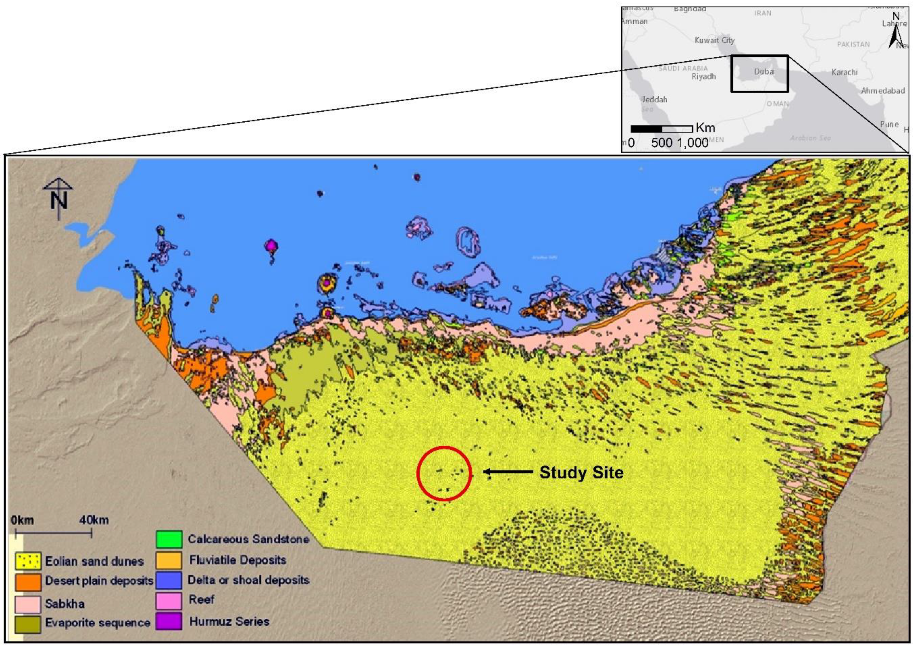
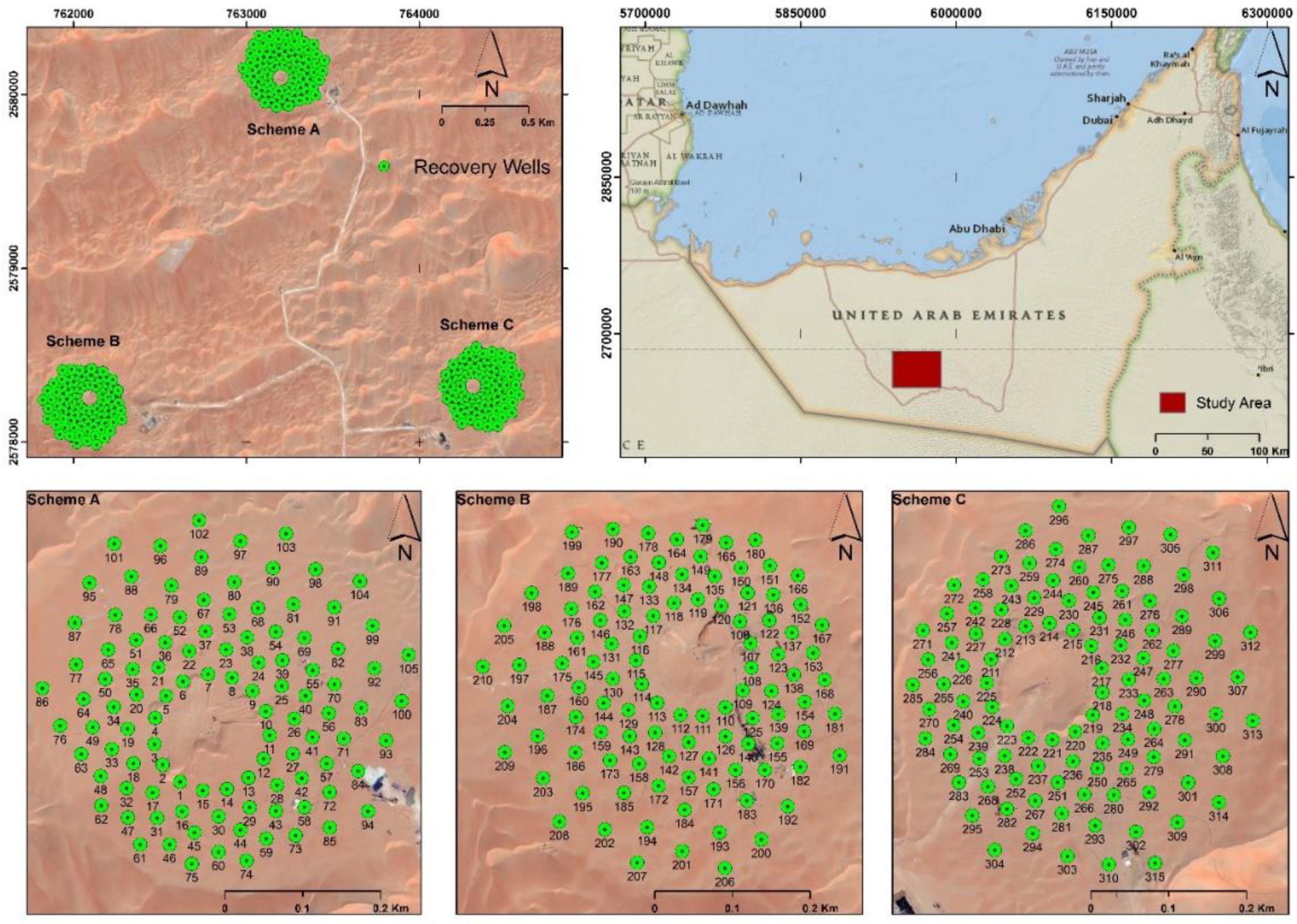
2.1. Study Area

The study area is in the United Arab Emirates. The SWSR was performed in the Liwa region located 150 km southwest of Abu Dhabi City (United Arab Emirates) (Figure 1).

The majority of the Liwa region is covered by eolian sands. Coring and geophysical logs from local investigations indicate the presence of three main lithological units under the study site:

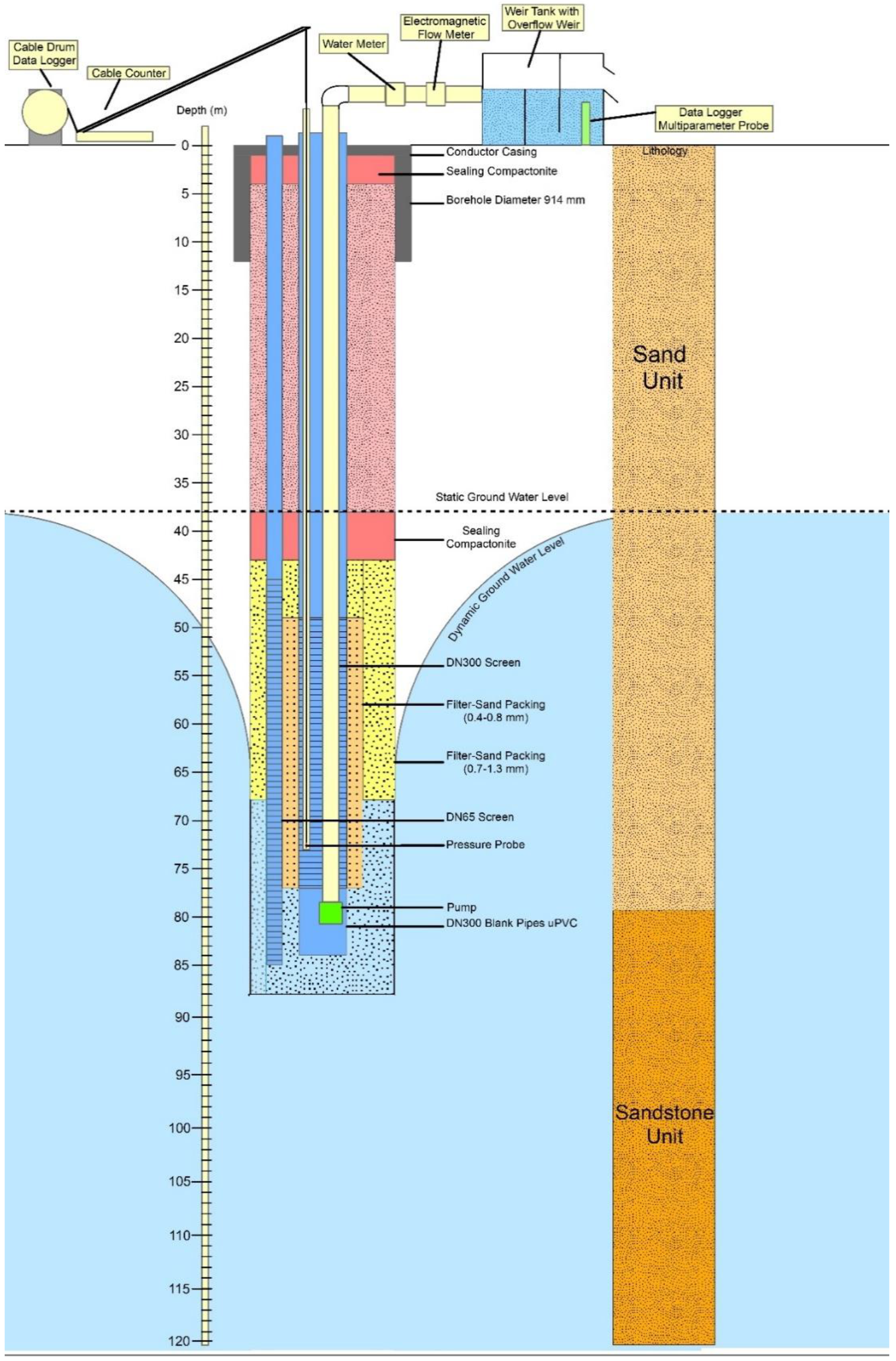
• The first unit consists of red-brown to yellowish-brown non-plastic, poorly graded, fine to medium, loose to very dense sand with trace silt. The water table is present within this unit. This layer exhibits varying degrees of cementation and consolidation that increase with depth. Zones of semi-consolidated and weakly to moderately cemented sand and sandstone may be observed throughout this layer particularly near the water table and near the bottom of this layer. The aquifer thickness is approximately 80 m.
• The sand unit is underlain by approximately 80 m thick yellowish-brown to reddish-brown to gray calcarenaceous semi-consolidated sand. It contains intercalation of siltstone, mudstone, marl, and thin sand lenses.
• The third unit consists of carbonates (light gray to white calcarenite, limestone, and dolomite) and gypsum located under the sandstone unit.

The aim of the project is to create a strategic water storage and recovery environment in the Liwa aquifer. To create a strategic water storage and recovery environment in the Liwa aquifer, 315 wells were installed and deployed in three different areas named Schemes A, B, and C, respectively. Each scheme is composed of 105 wells arranged in an approximate circular geometry of 25 ha (Figure 2).

2.2. Data and Well Design

SDTs were conducted for each well with incremented discharge rates of 30 m³/h, 60 m³/h, 90 m³/h, 120 m³/h, and 150 m³/h, respectively. Time duration of the steps was 3 h per 1 step. The data from each pumping test were obtained from multi-parameter probes at 1-min intervals with 10⁻³ m sensitivity. Each well was developed with one production pipe (DN300) and one monitoring pipe (DN65) (Figure 3).

Top hole of each well was drilled down to 11.4 m with 36” drill bit and the 30” conductor casing installed. After that, the wells were drilled down to an average of 80 m with 28” drill bit and a 11 4/5” diameter production pipe (DN300) string was installed. Monitoring pipe (DN65) was installed beside the production pipe (DN300). Before the installation, the lower 28 m of the production pipe were screened for each recovery well. The screened part of the wells thus taps the sandy formation only. Three multi-parameter probes were used in each well located above the pump, below the pump, and in the monitoring pipe DN65. Probes recorded temperature, electrical conductivity, and head pressure. Discharge rate was recorded using an electromagnetic flow meter for each well. The probe at weir tank recorded the electrical conductivity, temperature, and tank level. An example set of SDT data is given in Figure 4.

Figure 4A shows the sequencing of the 5 steps, the variation of the discharge rate and the drawdown evolution at each step. The plot of drawdown vs. logt (Figure 4B) indicates a linear evolution of the drawdown in accordance with Jacob’s assumption.

2.3. Methodology

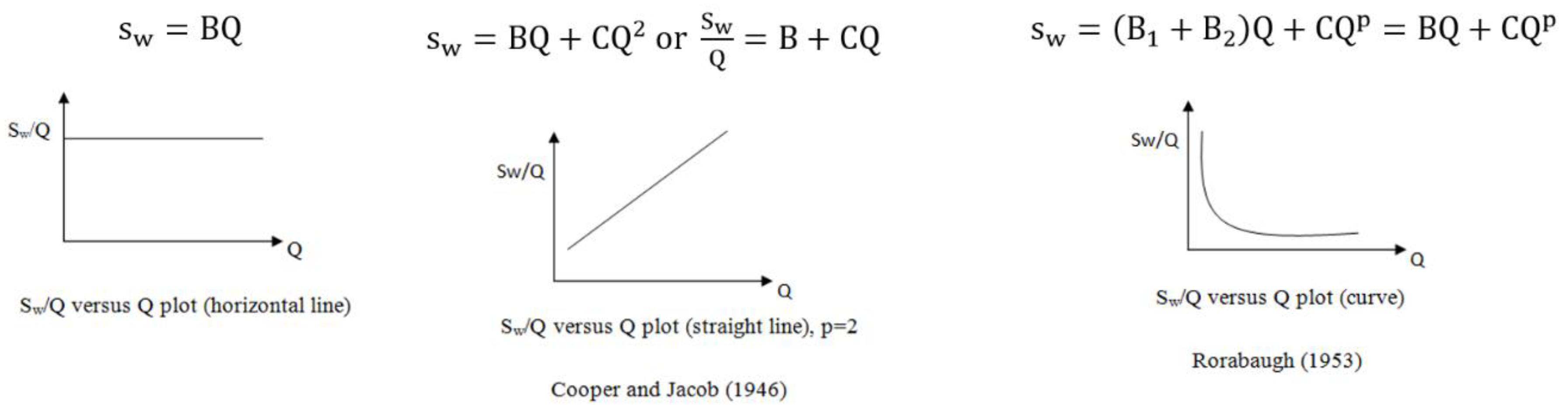
2.3.1. Literature Review

The procedure of changing pumping rates over a consistent time interval in a deliberate manner is known as a SDT. This is a single-well test where the initial pumping rate is lower than the maximum expected rate. After the drawdown stabilizes, then the rate is increased, or stepped up, to a higher rate for the same amount of time, usually 1 to 3 h [3].

Drawdown in a pumping well (S_w) is composed of two components, the aquifer loss (S₁) and the well loss (S_t).

S_w = S₁ + S_t

(1)

The aquifer loss (S₁) conforms to the laminar condition required by the Darcy law and is proportional to the discharge rate. The second drawdown component, the well loss S_t, is caused by the flow through the gravel pack, the well screen, and flow inside the well to the pump intake. Expressions of all these sub-components included in the well loss can be found in the literature [10]. Therefore, the well loss (S_t) is broken in two parts, a darcian well loss (S₂) and a turbulent well loss (S₃):

S_t = S₂ + S₃

(2)

The turbulent well loss is caused by high flow velocity close to the discharging well in the gravel pack and inside the well. Because of these difficulties, two models have been proposed in the literature and are widely used to express the total drawdown S_w in a discharging well. Jacob (1947) [2] first proposed the formula in Equation (3) to estimate the drawdown (S_w) in a pumping well:

S_w = BQ + CQ²

(3)

where S_w is the drawdown (L), Q (L³/T) is the discharge rate, B is the linear aquifer-loss coefficient (T/L²), C is the non-linear well-loss coefficient (T²/L⁵), BQ (L) is the linear fraction of the drawdown in the well termed “aquifer loss” and CQ² (L) is the non-linear fraction termed “well-loss”.

Rorabaugh (1953) [1] modified Jacob’s equation and suggested a more general form of Equation (3), substituting the well-loss exponent value of 2 by a variable p (Equation (4)). He showed that p was greater than 2, between 2.4 and 2.8 and averaged 2.5. Equation (4) is expressed as follows:

S_w = BQ + CQ^p

(4)

where p is the exponent parameter. Equation (2) is a more generalized form of the total drawdown.

In these equations, the coefficient B can be broken in two parts:

B = B₁ + B₂

(5)

where B₁ is the linear aquifer-loss coefficient and B₂ is the linear well-loss coefficient.

The total drawdown can be expressed as:

S_w = S₁ + S₂ + S₃

(6)

and

S₁ = B₁Q

(7)

S₂ = B₂Q

(8)

S₃ = CQ^p

(9)

In practice, it is seldom possible to separate B1 and B2 [10]. Thus, Jacob and Rorabaugh equations (Equations (3) and (4)) represent a simplification of the real flow conditions through and in the well. Both equations are still widely used to analyze SDT and may be applied to confined, unconfined, and leaky aquifers.

Well performance is usually defined, for a given discharge rate, as the ratio expressed in percent, between the theoretical linear drawdown BQ and the actual drawdown measured in the well S_w. The well efficiency issue has been the subject of much debate in the literature, since groundwater is mainly extracted by wells. Many methods are thus available to analyze SDT, estimate the parameters B, C, and p, and to determine the well efficiency.

When p is assumed to be equal to 2, Hantush–Bierschenk graphical method [11,12] is the most widely used procedure to estimate the parameters B and C. It consists to plot on an arithmetic paper the specific drawdown (S_w/Q) vs. the discharge (Q). The data should fall on a straight line, giving estimates of B (y-intercept for x = 0) and C (slope of the straight line).

When p is different than 2, the parameters B, C, and p, of Equation (4) can be estimated using the Rorabaugh trial-and-error straight line method [13]. The procedure is outlined below.

Walton (1962) [4] stated that the well efficiency is possible to determine using the non-linear well-loss coefficient (C) when p equals 2. He presented a set of criteria that suggested the following terms, with time is in second and length in meter:

• If C is less than 1800 s²/m⁵, the well is properly developed and designed,
• If C is ranged from 1800 s²/m⁵ to 3600 s²/m⁵, the well has a mild deterioration,
• If C is greater than 3600 s²/m⁵, the well has a severe clogging.

In addition to Hantush–Bierschenk graphical method and Rorabaugh trial-and-error method, several other graphical and computer-based methods have been proposed in the literature to analyze SDTs. Sheahan (1971) [14] proposed a set of type-curves to estimate the coefficients of Rorabaugh equation (Equation (4)). Eden and Hazel (1973) [15] presented a graphical method for confined aquifers based on the Cooper–Jacob approximation [16] for non-steady radial flow to a well, combined with Jacob’s equation (Equation (3)). Labadie and Helweg (1975) [17] argued that the graphical approach is unwieldy and proposed a computer code to analyze SDTs, by minimizing the least-square of the errors. Miller and Weber (1983) [18] developed an iterative method to solve Equation (2). Gupta (1989) [19] also proposed an interactive computer code to estimate parameters of Equation (2). Avci (1992) [20] developed an approach dealing with time varying data and variable time steps. Yeh (1989) [21] determined aquifer constant and well-loss constant based on non-graphical Newton’s method. Helweg (1994) [22] presented a solution for step drawdown test due to insufficient criteria of the Jacob (1947) equation. Kawecki (1995) [23] presented a procedure to determine the well performance. Recently, Van Tonder et al. (2001) [24], Singh (2002) [25] and Karami and Younger (2002) [26] analyze well performance calculations under different pumping well conditions.

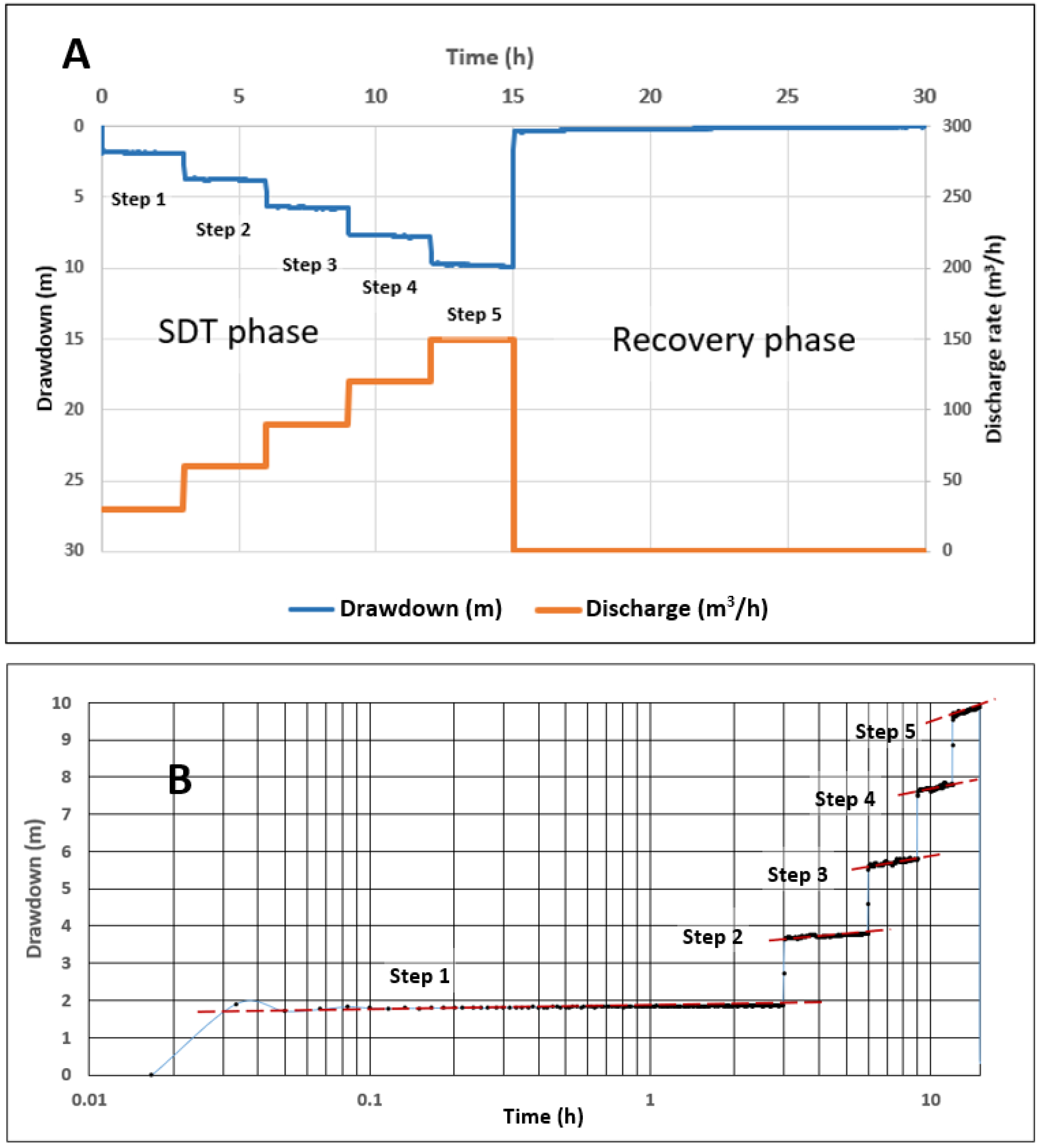
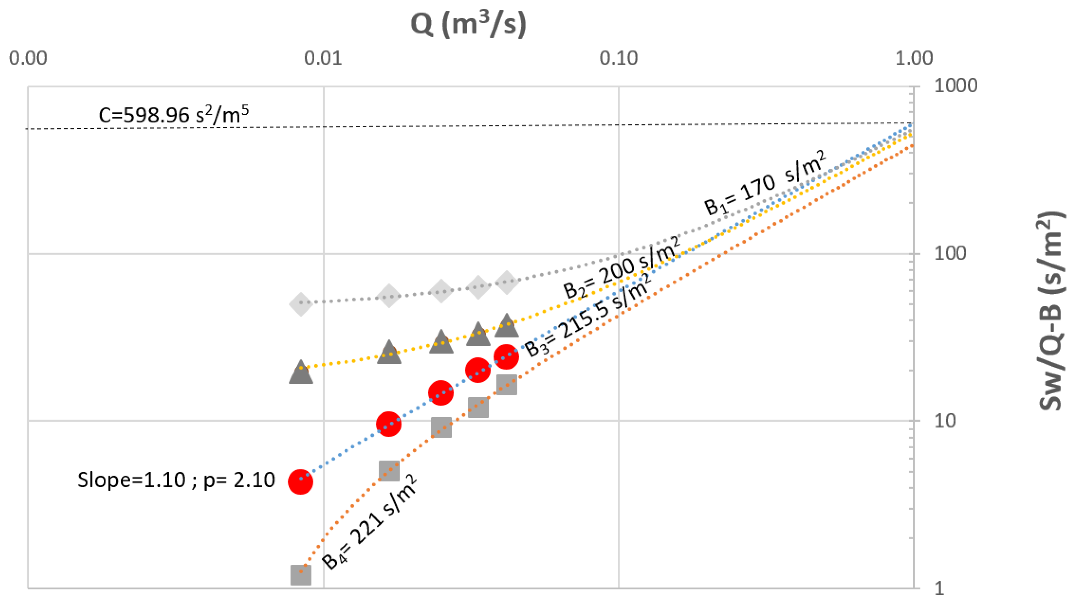
2.3.2. Application of Rorabaugh’s Trial-And-Error Method

Step drawdown tests are performed to yield the parameters B and C of Equation (3), or the parameters B, C, and p of Equation (4). Usually, diagnostic plots are used to evaluate these well-loss parameters. Values of S_w/Q versus Q are plotted, where S_w represents the drawdown at the end of each step. Various configurations of diagnostic plots are then possible to calculate the parameters of the drawdown Equation (3) or (4) and the well efficiency coefficient (Figure 5).

In this study, considering its generality and wider scope, Rorabaugh solution, Equation (4) was applied to calculate the coefficients B, C, and p for all 290 wells. When p ≠ 2, the values of B, C, and p cannot be found directly from the diagnostic plot of S_w/Q versus Q. Rorabaugh (1953) [1] proposed a trial-and-error approach to solve Equation (4) for B, C, and p. This approach is detailed in Boonstra (1999) [27] and summarized below.

Equation (4) can be rewritten as:

S_w/Q = B + CQ^p−1

(10)

Using a logarithmic transform, Equation (10) can be expressed as:

Log(S_w/Q − B) = logC + (p − 1)logQ

(11)

A plot of (Sw/Q − B) vs. Q on a log-log paper would provide a straight line for the correct value of B. The slope of the line is equal to (p − 1) from which p can be obtained. Intercept of the straight line with the Q = 1 axis gives the value of C. The Rorabaugh trial-and-error method consists of using manually different values of B until obtaining a straight line. This procedure becomes however tedious when a big amount of data must be analyzed, as in this study. Thus, this procedure was improved based on an automated iterative approach as shown in Figure 5. The procedure starts with an approximate value of B and plots the calculated points (Sw/Q − B; Q) on a log-log paper (Figure 6). Values of B are gradually modified, until the plotted points exhibit a straight line. The value of B satisfying these conditions is selected. The slope of the straight line is calculated, using the selected B value and the data (Swi, Qi) of the five steps of the SDT:

$$\frac{\Delta \log (\frac{{\mathrm{S}}_{\mathrm{w}}}{\mathrm{Q}}-\mathrm{B})}{\Delta \mathrm{logQ}}=\frac{\log ⎣(\frac{{\mathrm{S}}_{\mathrm{w}1}}{{\mathrm{Q}}_1}-\mathrm{B})/(\frac{{\mathrm{S}}_{\mathrm{w}5}}{{\mathrm{Q}}_5}-\mathrm{B})⎦}{\log (\frac{{\mathrm{Q}}_1}{{\mathrm{Q}}_5})}$$

(12)

This simple procedure speeds up considerably the determination of the non-linear model parameters, compared to a manual approach.

3. Results

3.1. Results Using Rorabaugh Solution

Using the automated iterative procedure outlined above, all 290 SDTs were analyzed to assess the parameters B, C, and p of Equation (4) and to determine the wells efficiency. The frequency distribution of the parameter p, on which there is much debate in the literature, is shown in Figure 7 and its statistics are reported in

Table 1. Statistics of the parameter p.

Average	Standard Deviation	Maximum Value	Minimum Value
1.71	0.78	6.01	0.35

.

The statistics (Table 1) show that the range of p values is quite extensive. The minimum is 0.35 and the maximum 6.01. This result is quite novel, since to date such variability in p values has not yet been demonstrated. This also implies that Jacob’s model is often inapplicable. The frequency distribution of p values is displayed in Figure 7. The shape is asymmetrical, with a positive asymmetry. These features are confirmed when plotting p values on a probability diagram (Figure 8). It can be deduced that p behaves like a lognormal variable. The frequency diagram (Figure 7) indicates that only 45% of p values are close to 2 (Classes between 1.8 and 2.2). Thus, only 45% of the SDT could have been correctly analyzed using Jacob’s model.

Statistics of the well-loss coefficient C are shown in

Table 2. Statistics of the well-loss coefficient C.

Average	Standard Deviation	Maximum Value	Minimum Value
3.04 × 106	4.60 × 107	7.81 × 108	1.88 × 10−1

. They reveal that the variability of this parameter is extremely high. The standard deviation is higher than the average.

As in Rorabaugh’s model the well-loss coefficient C and the exponent p are related to each other, and taking advantage of the exceptional large database available, an analysis of the relationship between these parameters was performed. Figure 9 shows the plot of p values versus C values in a semi-logarithmic diagram. A significant positive relation of p vs. logC, with a determination coefficient R² of 0.83, is highlighted. This result shows that p is closely associated with parameter C. It cannot be constant, which calls again into question the model of Jacob.

Equation linking both parameters is given below:

p = 0.2315 × lnC + 0.5838

(13)

where C is expressed in s²/m⁵.

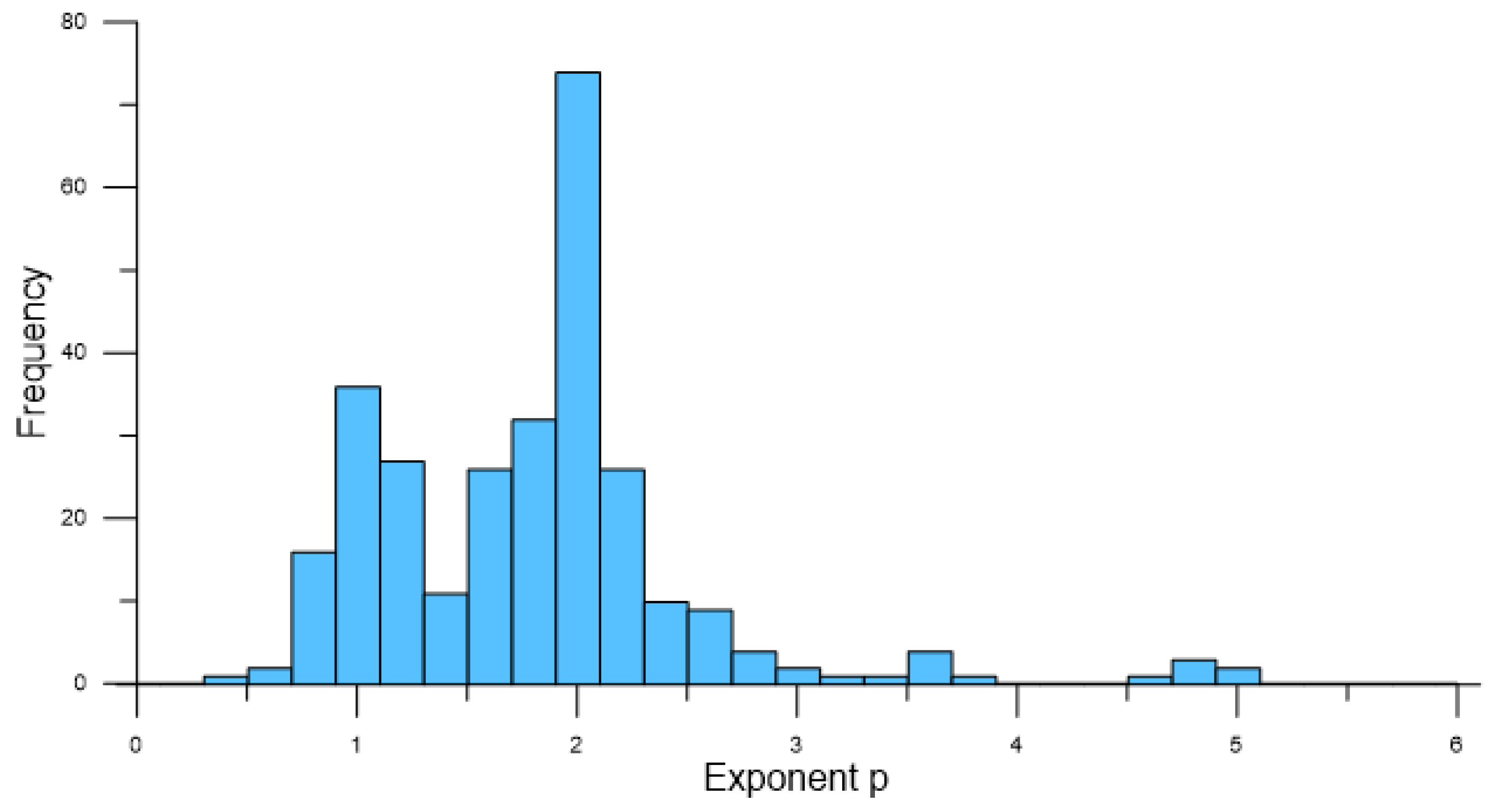
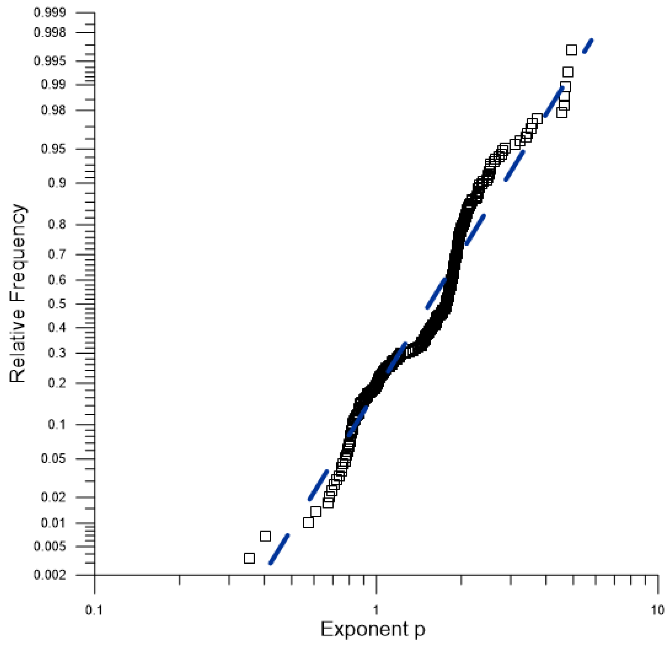
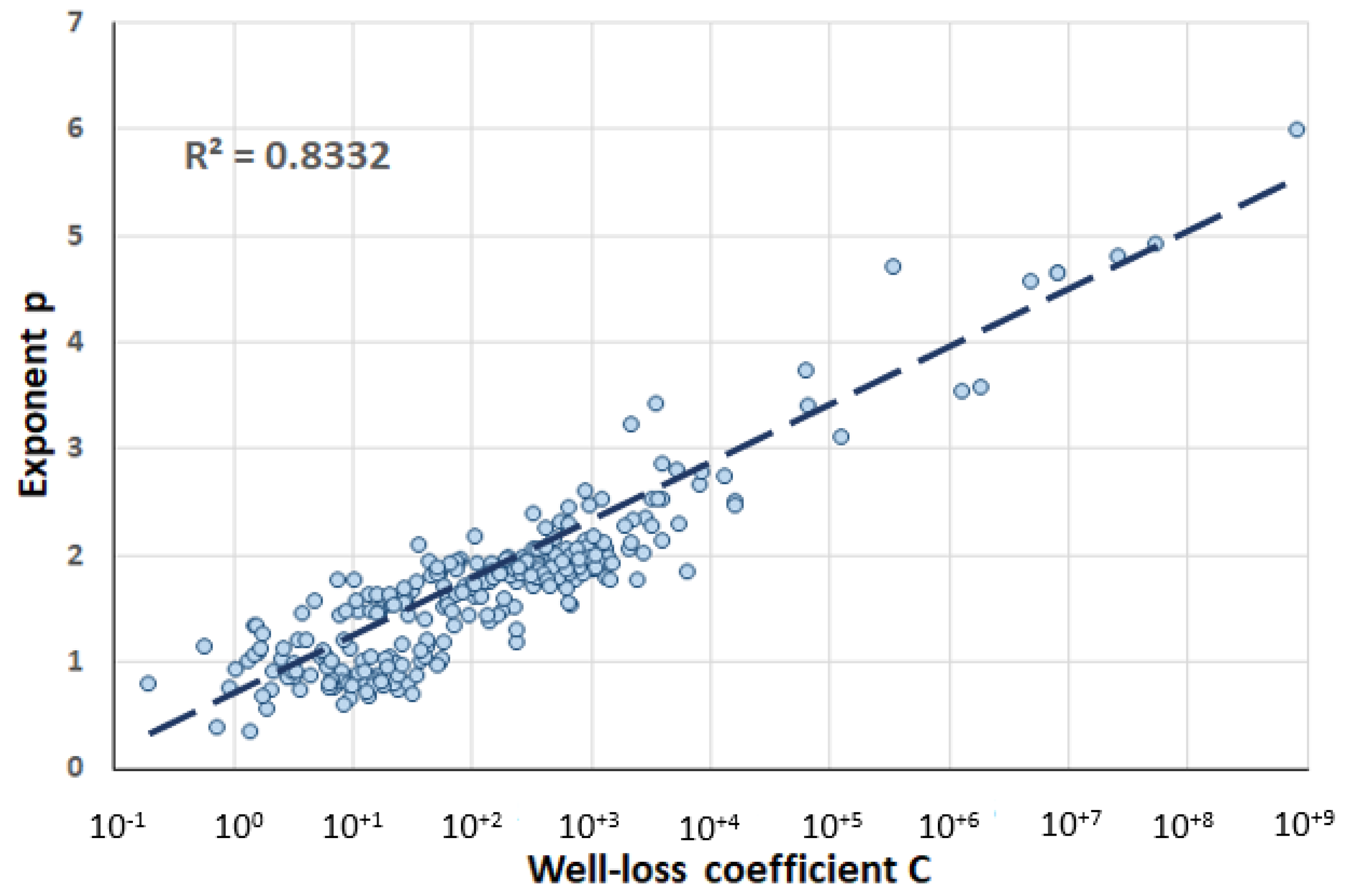
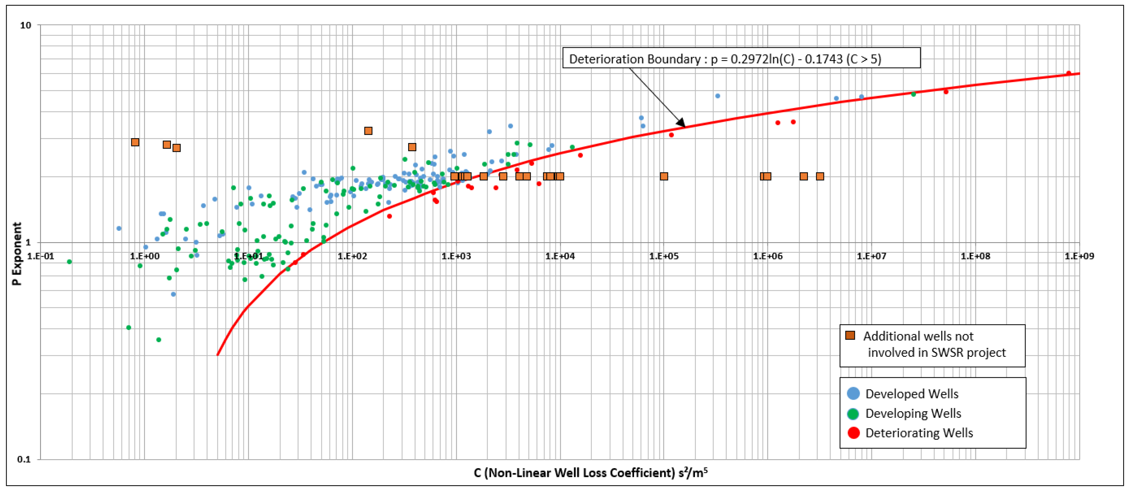
3.2. Development of a General Well Efficiency Criteria (GWEC)

Using the database of the Rorabaugh’s equation parameters (Equation (4)), the well efficiency was estimated for each of the 290 wells. Accordingly, the wells were classified in three groups: developed wells, developing wells, non-properly designed (or deteriorating) wells. These classified wells are plotted in a log-log diagram of the exponent p vs. well-loss coefficient C (Figure 10). This diagram clearly discriminates the deteriorating non-properly developed wells from the developed or developing wells. A boundary could be delineated on the diagram, differentiating between deteriorating and developed/developing wells. Equation of this deteriorating boundary is:

p = 0.2972 × lnC − 0.1743 (C > 5)

(14)

where units used to express C are m and s. The Equation (14) holds for C > 5, as for values of C less than 5, non-linear well losses are minor compared to linear darcian losses.

The red curve in Figure 10 represents the boundary curve. On the upper part from the red curve, the wells are “properly designed and developed”. On the lower part from the red curve they are “deteriorating”. Considering the very large range of the exponent p values, this procedure would permit assessment of the efficiency of any well, which has been analyzed by a step drawdown test. Accordingly, it was termed as General Well Efficiency Criteria (GWEC). Using GWEC results, out of total 290 wells, 270 wells are classified as developed or developing wells. The remaining 20 wells are in deteriorating condition.

The GWEC (Figure 10) shows that the region below the deterioration curve represents the minimum and maximum limits of C values with allowable p ranges. This allowed to defined intervals of the exponent p and the well-loss coefficient, associated with wells categories (developed/developing wells; deteriorating wells). These intervals are reported in

Table 3. Tabulated General Well Efficiency Criteria (GWEC).

Exponent p	Developed or Developing Wells	Wells in Deteriorating Condition
1–2	C < 1800	C > 1800
2–3	C < 4 × 104	C > 4 × 104
3–4	C < 2 × 106	C > 2 × 106
4–5	C < 5 × 107	C > 5 × 107
5–6	C < 8 × 108	C > 8 × 108

C: Non-Linear Well-Loss Coefficient (s^p/m^3p−1).

. The use of the tabulated form of GWEC in Table 3 is thus straightforward to assess the well performance.

To assess the generality of this criteria, several SDT results were collected from the literature [4,12,14,15,17,20,23,27,28,29,30,31,32,33,34,35,36]. These SDTs are related to pumping tests performed in various hydrogeological environments (alluvial aquifers, sand-gravel aquifers, carbonate/karstified aquifers, volcanic aquifers) in various countries (France, East Africa, USA, Poland, Iraq, Iran, Slovenia). The data from these tests (p and C) are plotted in Figure 10 but do not intervene in any way in designing the deterioration boundary curve. The plot clearly shows that the boundary deterioration curve without contest differentiates deteriorating wells from developed/developing wells, in accordance with the conclusions of these studies.

4. Conclusion

SDTs are performed to assess pumping well performance. Interpretation of SDTs is usually done using the Jacob model or the more generalized Rorabaugh model. There is much debate in the literature on the parameters of these models. The large and unique database, assembled within the SWSR Project in Abu Dhabi, allowed a rigorous and thorough analysis of the parameters of Rorabaugh’s model. This study resulted in novel findings. First it was shown that the range of exponent p values is much more extensive compared to what is proposed in the literature. In addition, p behaves like a lognormal variable. The study also revealed that the exponent p and the well-loss coefficient C are closely associated, implying that p is not constant. This calls into question the Jacob model where p is constant and equal to 2.

A graphical and tabulated procedure, termed GWEC, is finally proposed, which allows assessment of the well performance (developed/developing well; deteriorating well) based on the values of the exponent p and the well-loss coefficient C, derived from Rorabaugh’s model. Generality of this criteria has been validated using additional data (p, C) collected from the literature, related to various hydrogeological environments in several countries. Lognormality of the exponent p further supports the general scope of this procedure.

References

1. Rorabaugh, M.I. Graphical and Theoretical Analysis of Step-Drawdown Test of Artesian Wells. Proc. Am. Soc. Civ. Eng. 1953, 19, 1–23. [Google Scholar]
2. Jacob, C.E. Drawdown Test to Determine Effective Radius of Artesian Well. Trans. Am. Soc. Civ. Eng. 1947, 112, 1047–1070. [Google Scholar]
3. Clark, L. The Analysis and Planning of Step Drawdown Tests. Q. J. Eng. Geol. Hydrogeol. 1977, 10, 125–143. [Google Scholar] [CrossRef]
4. Walton, W.C. Selected Analytical Methods for Well and Aquifer Evaluation. Ill. State Water Surv. Bull. 1962, 49, 81. [Google Scholar]
5. Bierschenk, W.H.; Wilson, G.R. The exploration and development of groundwater resources in Iran. IAHS Publ. 1961, 2, 607–627. [Google Scholar]
6. Lennox, D.H. Analysis of Step-Drawdown Test. J. Hydraul. Div. Proc. Am. Soc. Civ. Eng. 1966, 92, 25–48. [Google Scholar]
7. Duffield, G.M. AQTESOLV for Windows Version 4.5 User’s Guide. 2007. Available online: http://www.aqtesolv.com/download/aqtw20070719.pdf (accessed on 1 December 2017).
8. Rumbaugh, D.B.; Rumbaugh, J.O. Guide to Using AquiferWin32. Environmental Simulations Inc., 2011. Available online: http://www.groundwatersoftware.com/ftp/aquiferwin32-4.pdf (accessed on 1 December 2017).
9. Waterloo Hydrogeologic Inc. Aquifertest Pro User’s Manual: Graphical Analysis and Reporting of Pumping and Slug Test Data. 2002. Available online: https://www.waterloohydrogeologic.com/aquifertes (accessed on 1 December 2017).
10. Misstear, B.; Banks, D.; Clark, L. Water Wells and Boreholes, 2nd ed.; Wiley Blackwell: West Sussex, UK, 2017; p. 518. [Google Scholar]
11. Hantush, S.M. Drawdown around wells of variable discharge. J. Geophys. Res. 1964, 69, 4221–4235. [Google Scholar] [CrossRef]
12. Bienrschek, W.H. Determining Well Efficiency by Multiple Step-Drawdown Tests; International Association of Scientific Hydrology: Wallingford, UK, 1963; pp. 493–507. [Google Scholar]
13. Kruseman, G.P.; de Ridder, N.A. Analysis and Evaluation of Pumping Test Data; International Institute for Land Reclamation and Improvement: Wageningen, The Netherland, 1994; p. 372. [Google Scholar]
14. Sheahan, N.T. Type Curve Solution of Step Drawdown Test. Groundwater 1971, 9, 25–99. [Google Scholar] [CrossRef]
15. Eden, R.N.; Hazel, C.P. Computer and Graphical Analysis of Variable Discharge Pumping Tests of Wells; Institution of Engineers Australia: Barton, Australia, 1973; Volume 15, pp. 5–10. [Google Scholar]
16. Cooper, H.H.; Jacob, C.E. A Generalized Graphical Method for Evaluating Formation Constants and Summarizing Well Field History. Eos. Trans. AGU 1946, 27, 526–534. [Google Scholar] [CrossRef]
17. Labadie, J.W.; Helweg, O.J. Step-drawdown Test Analysis by Computer. Groundwater 1975, 13, 438–444. [Google Scholar] [CrossRef]
18. Miller, C.T.; Weber, W.J. Rapid solution of the non-linear step-drawdown equation. Groundwater 1984, 21, 584–588. [Google Scholar] [CrossRef]
19. Gupta, A.D. On Analysis of Step-Drawdown Data. Groundwater 1989, 27, 874–881. [Google Scholar] [CrossRef]
20. Avci, C.B. Parameter Estimation for Step-Drawdown Tests. Groundwater 1992, 30, 338–342. [Google Scholar] [CrossRef]
21. Yeh, H.D.; Han, H.Y. Numerical Identification of Parameters in Leaky Aquifers. Groundwater 1989, 27, 655–663. [Google Scholar] [CrossRef]
22. Helweg, O.J. A General Solution to the Step-Drawdown Test. Groundwater 1994, 32, 363–366. [Google Scholar] [CrossRef]
23. Kawecki, M.W. Meaningful Estimates of Step-Drawdown Tests. Groundwater 1995, 33, 23–32. [Google Scholar] [CrossRef]
24. Van Tonder, G.J.; Botha, J.F.; Chiang, W.H.; Kunstmann, H.; Xu, Y. Estimation of the Sustainable Yields of Boreholes in Fractured Rock Formations. J. Hydrol. 2001, 241, 70–90. [Google Scholar] [CrossRef]
25. Singh, S.K. Aquifer Boundaries and Parameter Identification Simplified. J. Hydraul. Eng. 2002, 128, 774–780. [Google Scholar] [CrossRef]
26. Karami, G.H.; Younger, P.L. Analysing Step-Drawdown Tests In Heterogeneous Aquifers. Q. J. Eng. Geol. Hydrogeol. 2002, 35, 295–303. [Google Scholar] [CrossRef]
27. Boonstra, J. Well Design and Construction. In The Handbook of Groundwater Engineering; Delleur, J.W., Ed.; CRC Press LLC: Boca Raton, FL, USA, 1999. [Google Scholar]
28. Castany, G. Principles et méthodes de l’hydrogéologie [Hydrogeology: Principles and methods]; Dunod: Paris, France, 1982; p. 238. [Google Scholar]
29. Jalludin, M.; Razack, M. Assessment of hydraulic properties of sedimentary and volcanic aquifer systems under arid conditions in the Republic of Djibouti (Horn of Africa). Hydrogeol. J. 2004, 12, 159–170. [Google Scholar] [CrossRef]
30. Ginger Env. & Infrasturctures. Interprétation du Pompage D’essai. 2009. Available online: http://doc-oai.eaurmc.fr/cindocoai/.../2999/.../rapport_essai%20de%20pompage.PDF_862K (accessed on 2 July 2019).
31. Mawlood, D.K.; Mustafa, J.S. Analysis of Well Losses and Aquifer Losses on Pumping Test Results. ZANCO J. Pure Appl. Sci. 2016, 28, 61–67. [Google Scholar]
32. Spane, F.A.; Newcomer, D.R. Field Test Report: Preliminary Aquifer Test Characterization Results for Well 299-W15-225. US Department of Energy, Pacific Northwest National Laboratory, 2009. Available online: www.pnl.gov/main/publications/external/.../pnnl-18732.pdf (accessed on 2 July 2019).
33. Aqualinc Research Limited. Groundwater Report. Unpublished Report. Available online: https://api.ecan.govt.nz/TrimPublicAPI/documents/.../3277862/ (accessed on 2 July 2019).
34. Summa, G. A New Approach to the Step-Drawdown Test. 2009. Available online: https://arxiv.org/pdf/0903.4755 (accessed on 2 July 2019).
35. Krivic, P. Interprétation des essais par pompage réalisés dans un aquifère Karstique. Geologija 1983, 26, 149–186. [Google Scholar]
36. Polak, K.; Klich, J.; Kaznowska, K. The method of wells’ efficiency estimation. In Mine Water—Managing the Challenges, Proceedings of the 11th IMWA Congress 2011, Aachen, Germany, 4–11 September 2011; Rüde, T., Freund, A., Wolkersdorfer, C., Eds.; International Mine Water Association: Sydney, NS, Canada, 2011; pp. 153–157. [Google Scholar]
Figure 1. Location and geological map of the study area. Geological map adapted from https://enviroportal.ead.ae/map/.
Water 11 01784 g001
Figure 2. The Strategic Water Storage and Recovery Project. Recovery well locations in three Schemes A, B, and C.
Water 11 01784 g002
Figure 3. Well Design of the Strategic Water Storage and Recovery Project.
Water 11 01784 g003
Figure 4. Example of step drawdown test (SDT) progress. Well RW002. (A) Arithmetic plot of the discharge rate and drawdown variation at each step. (B) Semi-logarithmic plot of drawdown vs. time, showing the evolution of drawdown during each step.
Water 11 01784 g004
Figure 5. Diagnostic plots and proper equations for well-loss coefficients [1,16].
Water 11 01784 g005
Figure 6. An Example of log-log plot of (Sw/Q − B) versus discharge (Q) to determine the well losses parameters B, C, and p according to the Rorabaugh (1953) [1] method. For the selected value of B (B = 215.5 s/m2), the plotted points exhibit a straight line. The slope of this line is 1.10, yielding the value of p = 2.10. Intersection of this line, with the vertical axis Q = 1, gives the value C = 598.96 s/m2.
Water 11 01784 g006
Figure 7. Frequency distribution of the parameter p values.
Water 11 01784 g007
Figure 8. Plot of the parameter p values on a probability diagram.
Water 11 01784 g008
Figure 9. Plot of the exponent p values vs. well-loss coefficient C values.
Water 11 01784 g009
Figure 10. General Well Efficiency Criteria. Exponent Parameter (p) vs. Non-Linear Well-Loss Coefficient (C) Graph. The wells involved in the SWSR project are represented by circles. Wells represented by brown squares are collected from the literature and used to assess the GWEC.
Water 11 01784 g010