Levantine Intermediate and Levantine Deep Water Formation: An Argo Float Study from 2001 to 2017
by
 , and
, and
Elisabeth Kubin
1,*, 
Pierre-Marie Poulain
1,2, 
Elena Mauri
1,
Milena Menna
1 and
and
Giulio Notarstefano
1 1
National Institute of Oceanography and Experimental Geophysics, OGS, 34010 Sgonico (TS), Italy
2
Centre for Maritime Research and Experimentation, CMRE, 19126 La Spezia, Italy
*
Author to whom correspondence should be addressed.
Water 2019, 11(9), 1781; https://doi.org/10.3390/w11091781
Submission received: 12 July 2019
/
Revised: 23 August 2019
/
Accepted: 23 August 2019
/
Published: 27 August 2019
(This article belongs to the Special Issue Ocean Exchange and Circulation)
Abstract
:Levantine intermediate water (LIW) is formed in the Levantine Sea (Eastern Mediterranean) and spreads throughout the Mediterranean at intermediate depths, following the general circulation. The LIW, characterized by high salinity and relatively high temperatures, is one of the main contributors of the Mediterranean Overturning Circulation and influences the mechanisms of deep water formation in the Western and Eastern Mediterranean sub-basins. In this study, the LIW and Levantine deep water (LDW) formation processes are investigated using Argo float data from 2001 to 2017 in the Northwestern Levantine Sea (NWLS), the larger area around Rhodes Gyre (RG). To find pronounced events of LIW and LDW formation, more than 800 Argo profiles were analyzed visually. Events of LIW and LDW formation captured by the Argo float data are compared to buoyancy, heat and freshwater fluxes, sea surface height (SSH), and sea surface temperature (SST). All pronounced events (with a mixed layer depth (MLD) deeper than 250 m) of dense water formation were characterized by low surface temperatures and strongly negative SSH. The formation of intermediate water with typical LIW characteristics (potential temperature > 15 °C, salinity > 39 psu) occurred mainly along the Northern coastline, while LDW formation (13.7 °C < potential temperature < 14.5 °C, 38.8 psu < salinity < 38.9 psu) occurred during strong convection events within temporary and strongly depressed mesoscale eddies in the center of RG. This study reveals and confirms the important contribution of boundary currents in ventilating the interior ocean and therefore underlines the need to rethink the drivers and contributors of the thermohaline circulation of the Mediterranean Sea.
1. Introduction
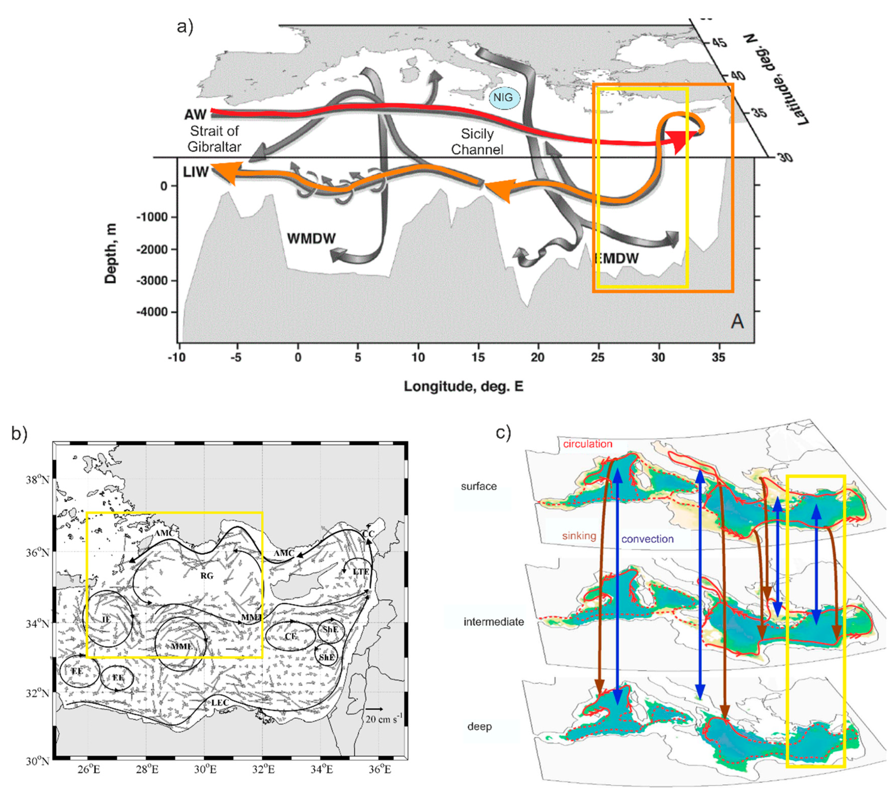
The Mediterranean Sea (Figure 1) is composed of two basins of nearly equal size, the Western and the Eastern Mediterranean Sea, connected by the Sicily Channel. The general circulation of the Mediterranean Sea can be divided into three dominant scales of motion: the basin scale including the thermohaline circulation, the sub-basin scale including permanent and quasipermanent cyclonic and anticyclonic gyres, and the mesoscale with small but energetic temporary eddies [1,2]. All these scales are interacting.
Through the Strait of Gibraltar, the relatively fresh Atlantic water (AW) enters the Western Mediterranean Sea within the upper 100 to 200 m. It is modified flowing eastward, passes the Sicily Channel and the Ionian Sea and enters the easternmost part of the Mediterranean, the Levantine Sea. The salinity of the AW in the Levantine Sea depends on the circulation patterns during its path, mainly influenced by the variability of the circulation of the North Ionian Gyre (NIG) which varies significantly at seasonal and decadal scales ([3,4,5]; Figure 1a).
Due to evaporation and air–sea exchanges, the AW is becoming saltier and warmer when reaching the Levantine Sea. The AW that enters the Levantine Sea is identified by a subsurface minimum of S < 38.6 psu and by a temperature of 14–15 °C. The Levantine intermediate water’s (LIW) properties are defined by salinity values greater than 39 psu, potential temperature values greater than 15 °C and potential density values between 29 and 29.05 kgm−3 while typical ranges for Levantine deep water (LDW) are 13.7–14.5 °C and 38.8–38.9 psu [6].
The strong advective surface salinity preconditioning [7] and buoyancy losses due to heat and freshwater fluxes in winter lead to dense water formation, sinking takes place, and the LIW is formed (Figure 1a). The LIW is characterized by a subsurface salinity maximum and occupies and moves in the intermediate layers between 200 and 600 m throughout the Mediterranean Sea until it reaches the Atlantic Ocean through the Strait of Gibraltar. Therefore, the LIW contributes as an important driver to the thermohaline circulation of the Mediterranean Sea. The specific pathways of the thermohaline circulation depend strongly on where and when the LIW is formed.
According to the prevailing view, the LIW formation takes place within the cyclonic Rhodes Gyre (RG) during the winter months ([1,8], Figure 1a). However, experimental studies showed that the RG is also a place of LDW formation and that the Levantine basin is a site of multiple and different water mass formation processes [6,9,10]. Furthermore, recent theoretical models revealed that no net mean sinking takes place within Mediterranean convection sites such as the RG, while boundary currents undergo net intense sinking ([11,12,13,14,15,16]; mean from 1980 to 2013 for all seasons; Figure 1c). This is due to vorticity dynamics: Only dissipation at the boundary (and bottom friction) can balance the vortex stretching that arises from vertical motions induced by net sinking.
The focus of this study is on the Northwestern Levantine Sea (NWLS; latitude: 33°–37°, longitude: 26°–32°; red rectangle in Figure 1b), the larger area around the RG, including also the area along the Northern coast. The NWLS is characterized by a general cyclonic surface circulation and the presence of the permanent RG, cyclonic and anticyclonic structures (such as Ierapetra (IG) and Mersa-Matruh Eddy (MME)), intense jets (such as the Mid Mediterranean Jet (MMJ); with minimum subsurface salinity values), a strong coastal current along the Northern coastline (the Asia Minor Current (AMC)), and the passage from the Cretan to the Levantine Sea ([17], Figure 1b).
This study aims to describe where and when LIW and LDW formation take place within the NWLS, using Lagrangian Argo float data over a period of 16 years. The results were compared to heat and freshwater fluxes and satellite data (SSH, SST).
Dense water formation processes occur on daily scales and are linked to temperature and salinity extrema which are not represented using climatological data sets or mixed layer depth (MLD) detection algorithms. Therefore, more than 800 Argo float profiles from 2001 to 2017 were analyzed visually to investigate LIW and LDW formation during winter months.
The paper is organized as follows: In Section 2, the data sets and analysis methods are presented. In Section 3, the time evolution of the heat and freshwater fluxes from 2001 to 2017 for the center of the RG are shown to identify periods of extreme heat losses due to outbreaks of strong cold and dry winds leading to dense water formation. Section 3 gives two examples of the LDW formation within the RG and one example of the typical LIW formation along the Northern coastline and characterizes the newly formed water masses. Section 4 gives an overall discussion and summarizes the major results of this work.
2. Datasets and Methods
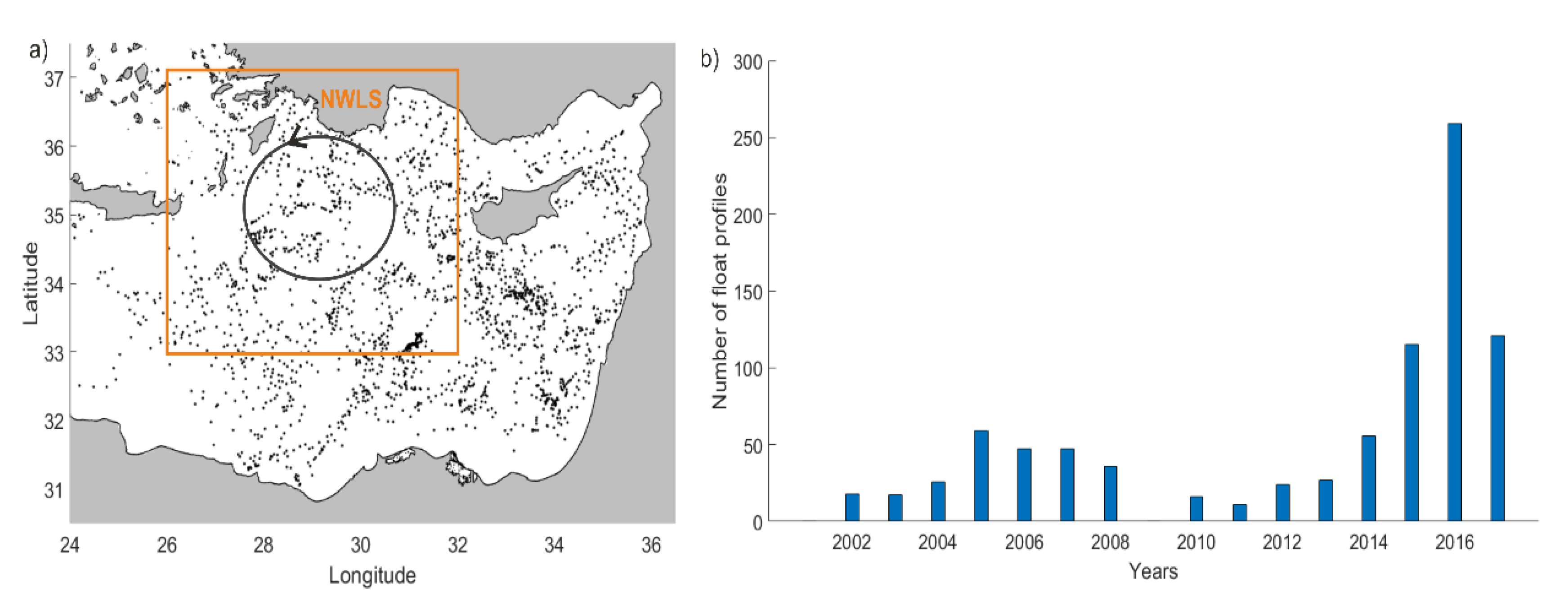
The datasets used for this study are Argo floats vertical profiles of temperature and salinity (T/S) collected in the NWLS during winter months (January, February, March—JFM) between 2001 and 2017. In total 879 T/S profiles from 20 floats were analyzed visually. Figure 2 shows the position of the Argo float profiles and the annual distribution of profiles for JFM between 2001 and 2017 for the area of study.
With the help of an external bladder, the Lagrangian floats descend to a programmed parking depth (350 or 1000 m) where they stay for a specified period (1–10 days, mainly 5 days [18]). Then, they descend to greater depths (up to 2000 m). During their ascent back to the surface, they measure temperature and salinity throughout the water column. At the surface they transmit the data to satellites and descend again. The transmitted data are stored at data assembly centers (DAC) which apply a quality control and provide open access to real time and delayed mode quality controlled data.
Quality controlled Argo float data were downloaded from the Ifremer Data Assembly Center (DAC; ftp://ftp.ifremer.fr/ifremer/argo/dac/coriolis/). For this study, only data with the best quality control (qc=1) were taken into account. Downloaded parameters included float number, position, time, pressure, temperature, and salinity.
Hydrographic properties were expressed as potential temperature, potential density, and salinity according to the practical salinity scale (PSU).
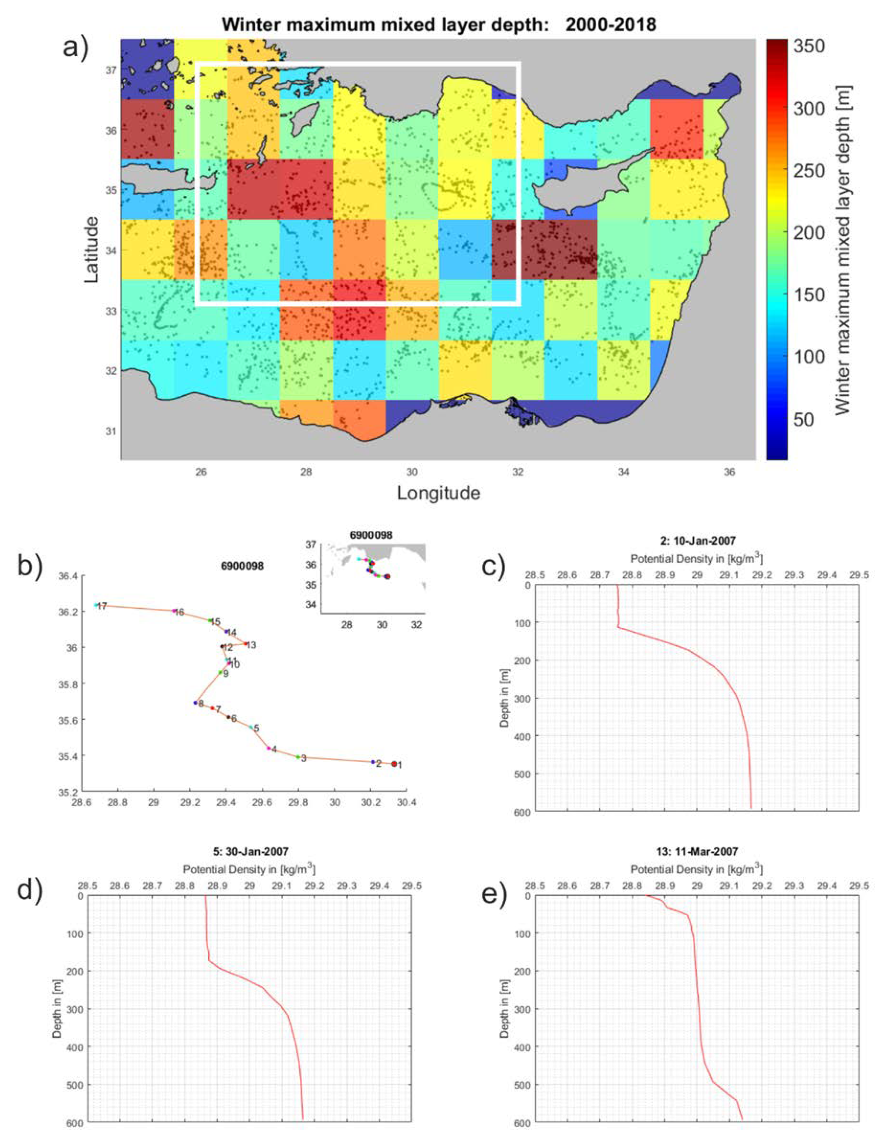
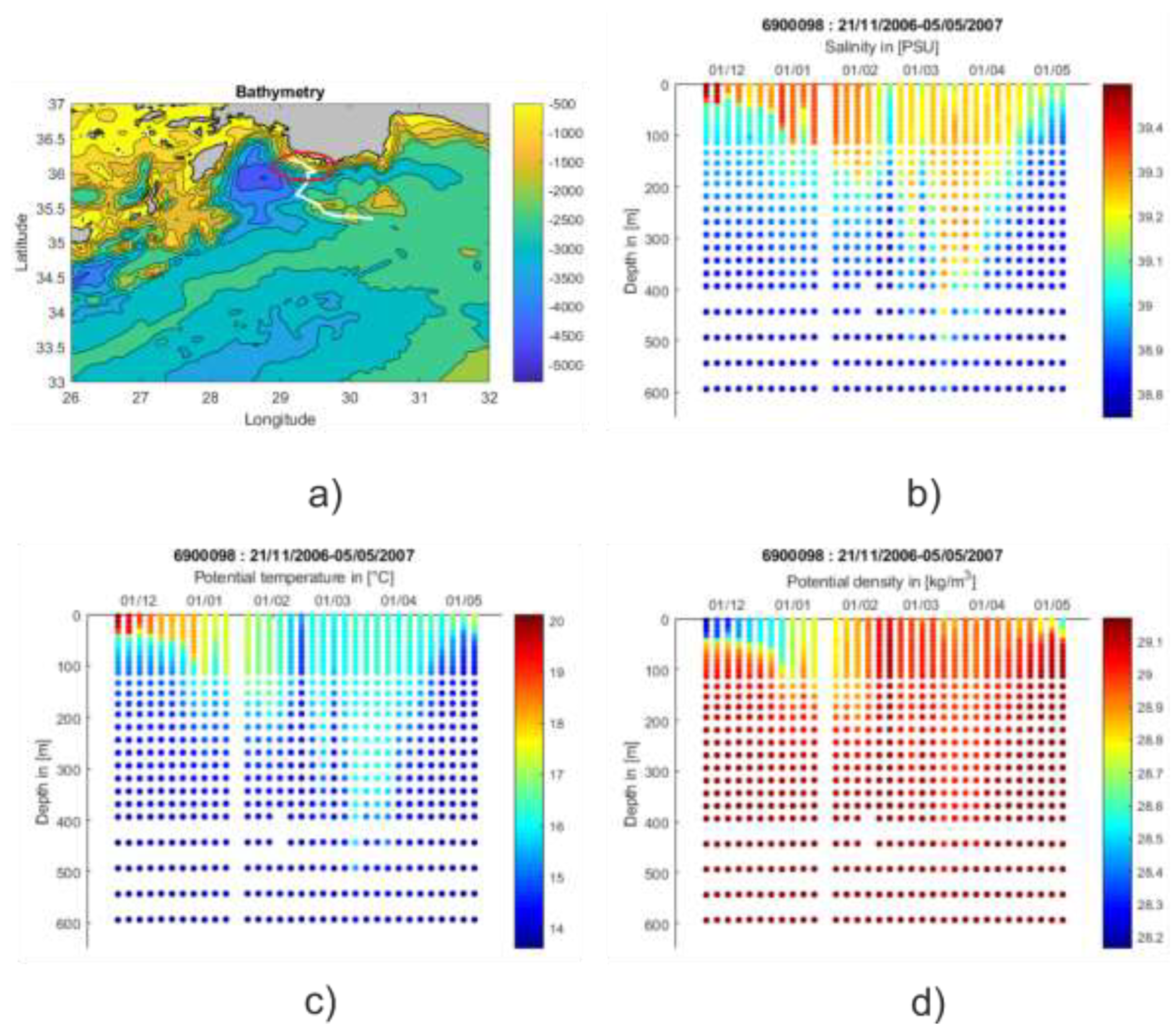
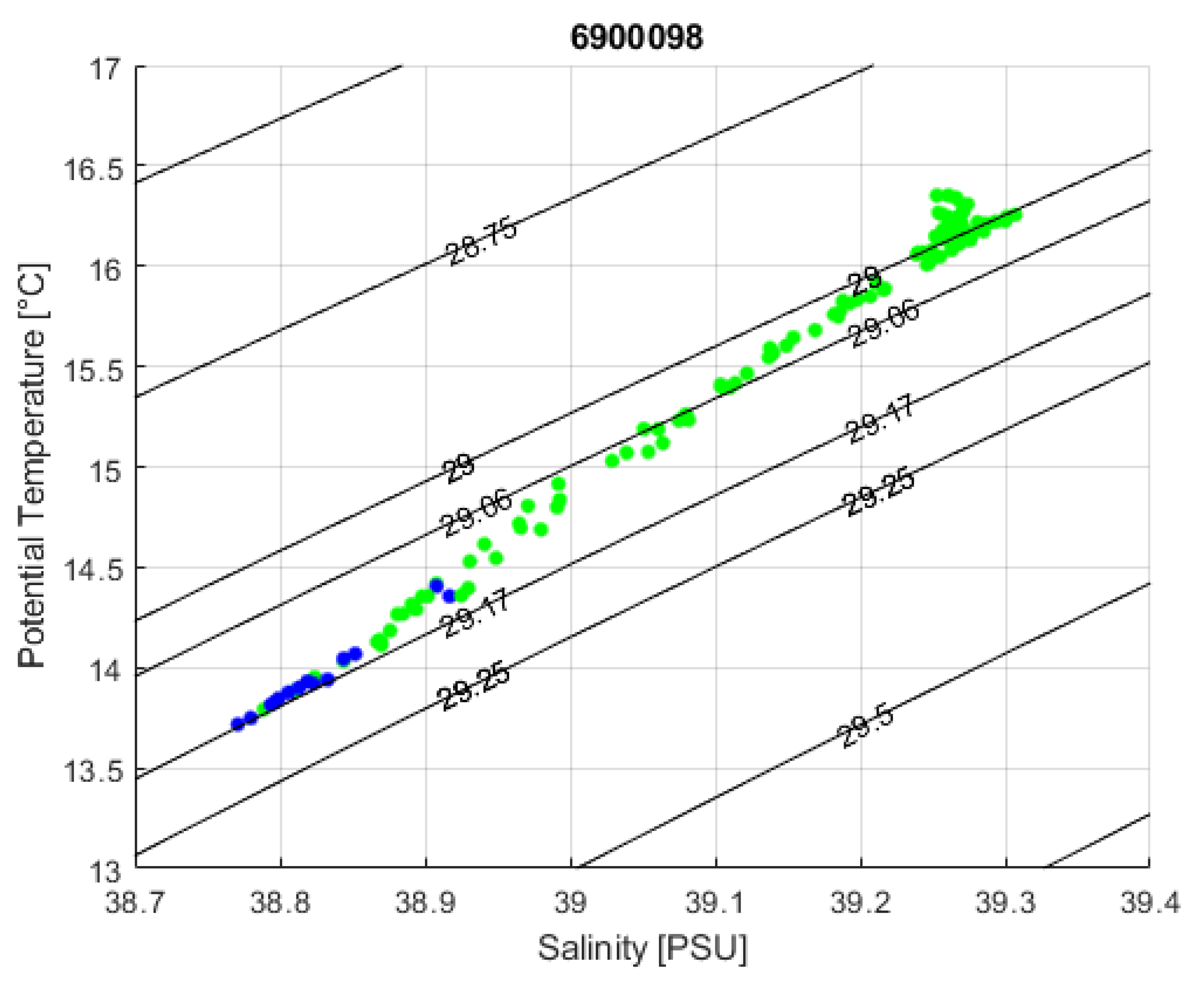
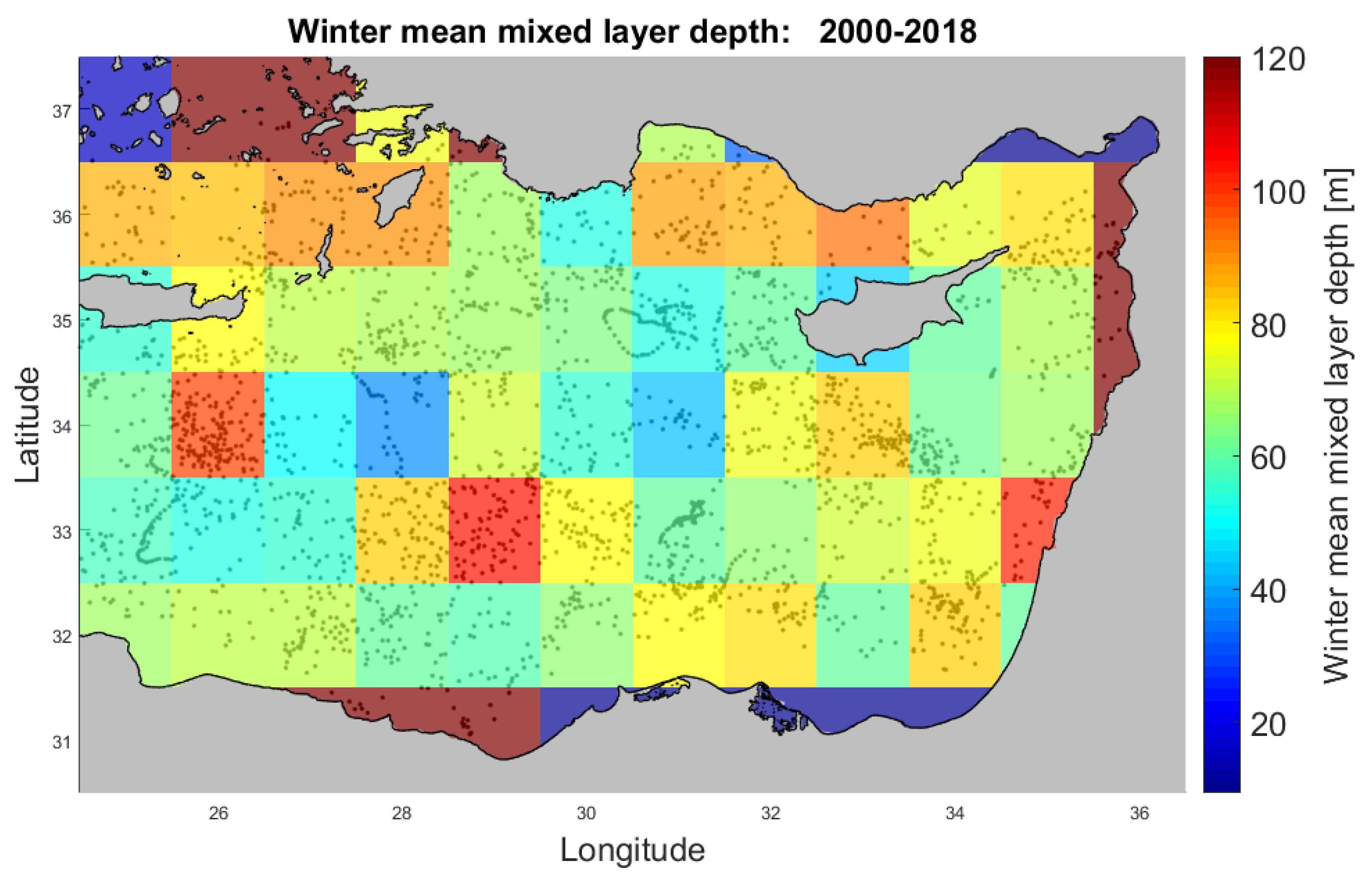
The visual inspection of the Argo float profiles is important due to the fact that the Argo floats may pass an area not exactly during the event of mixing or convection. They can instead sample days or weeks later when the recapping (i.e., a newly formed shallow MLD) already occurred. In such a case, MLD detection algorithms indicate a shallow MLD, but do not give any information about mixing or convection events before the recapping. While at the top, there can be already a newly formed MLD and the convection event can still be visible deeper in the water column. MLD detection statistics rarely give information about deep mixing events while the visual inspection of the form of the profile (potential temperature, salinity, and potential density) reveals clearly such events. Figure 3a shows the climatology of the winter maximum MLD derived from Argo float data and downloaded from [19] in the period 2000 to 2018. The maximum MLD is 225 m along the coastline of the NWLS (Figure 3a). The visual inspection of the Argo profiles in the same region reveals deeper dense water formation events. For example, in winter 2007, the float WMO 6900098 (Figure 3b), moving along the northern coastline of the NWLS, shows the deepening of the winter MLD from 100 m (Figure 3c) to 200 m (Figure 3d) in January. In March, when the maximum MLD is about 550 m, the recapping occurred (due to surface warming) with a newly formed MLD of about 50 m (Figure 3e). In this case, the MLD detention algorithm can fail, indicating the depth of 50 m as maximum MLD.
The SST and sea surface height (SSH) data were downloaded from Copernicus (marine.copernicus.eu). The interpolated SST product (SST_MED_SST_L4_NRT_OBSERVATIONS_010_004_c_V2) has a daily temporal resolution and a spatial resolution of 0.04° × 0.04°. The interpolated SSH product (SST_MED_SST_L4_REP_OBSERVATIONS_010_021) has a daily temporal resolution and a spatial resolution of 0.125° × 0.125°. Monthly means of SST superimposed with the geostrophic currents from SSH were used to describe the negative slope of eddies within the RG during intense convection events.
The freshwater fluxes were derived from ERA-INTERIM (daily) data. The downloaded parameters are evaporation (E) and total precipitation (P). The downloaded data have a time step of 12 hours, i.e., daily data at 00:00:00 and at 12:00:00 and a spatial resolution of 0.25° × 0.25°. The daily freshwater fluxes (FWF) were calculated as the subtraction of the daily means of E and P: FWF=E−P.
The air–sea heat fluxes were derived from ERA-INTERIM (daily) data. The downloaded parameters are: Surface net solar radiation (Qsw), surface net thermal radiation (Qlw), surface sensible heat flux (Qs), and surface latent heat flux (Ql). The heat budget can be expressed as the difference between the net shortwave solar radiation (incoming minus reflected) absorbed by the sea surface, the sum of the longwave back radiation, the sensible, the latent, and the advective heat flux. The advective heat flux (Qadv) was not available at ERA-INTERIM and therefore not considered. The downloaded data have a time step of 12 hours, i.e., daily data at 00:00:00 and at 12:00:00 and a spatial resolution of 0.25° × 0.25°. The daily mean of each parameter as well as the daily net heat fluxes were calculated as the sum of the daily means of each parameter: Qnet = Qsw + Qlw + Ql + Qs. The surface buoyancy flux B, composed by thermal (BT) and haline (BS) components, was calculated according to [20]:
where α is the thermal expansion coefficient, g = 9.8 ms−2 is the gravity acceleration, Cp = 3.9715 × 10⁻³ Jkg−1K−1 is the specific heat capacity of sea water, ρ0 = 1029 kgm−3 is a reference sea water density, β is the haline contraction coefficient and S0 = 38.9 is a reference salinity. α and β were calculated at surface pressure, using monthly mean surface salinity and monthly mean surface temperature, downloaded from Copernicus (MEDSEA_REANALYSIS_PHYS_006_004). B is positive when surface water gets lighter and negative when surface water becomes denser (river inputs as well as horizontal and vertical advection also contribute to density changes, but were not considered due to lack of data).
B = α × g × (Cp × ρ0)−1 × Qnet −β × S0 × g × (ρ0)−1 × (E−P)
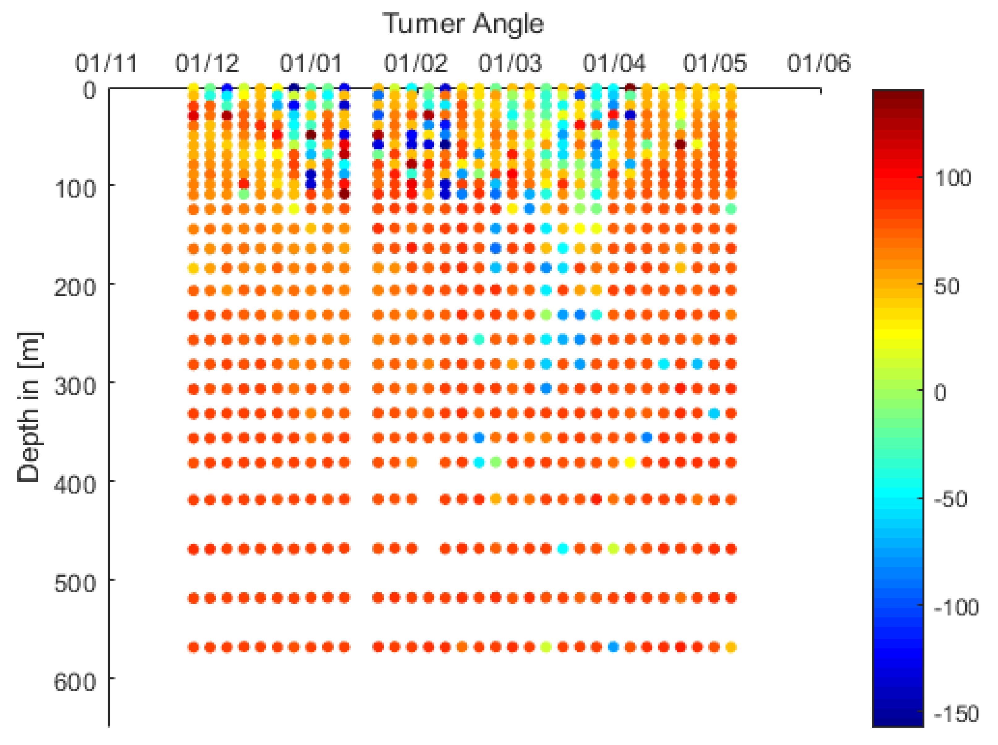
The Turner angle (Tu) was computed to evaluate the relative roles of temperature and salinity gradients on the density gradients. Tu is defined as the four-quadrant arctangent [21], which units are degrees of rotation and was calculated with the Gibbs-SeaWater (GSW) Oceanographic Toolbox [22]. Argo float salinity and temperature were converted to absolute salinity and to conservative temperature, respectively. The conservative temperature represents more accurately the heat content [22].
Tu = 45° indicates that temperature is the only contributor, while Tu = −45° indicates that salinity is the only contributor to density changes; |Tu|< 45° indicates stable stratification and in this condition both temperature and salinity contribute to the density change ; 45° < Tu < 90° shows that salinity is working against temperature and is also called the ‘salt finger regime’ with the strongest activity near 90°; −90° < Tu < −45° is called the ‘diffusive regime’ and shows that temperature is working against salinity, reaching the strongest activity near −90°; |Tu|> 90° characterizes a statically unstable water column (where the Brunt–Vaisalaa frequency N2 < 0).
3. Results
3.1. Heat and Freshwater Fluxes within the Northwestern Levantine Sea
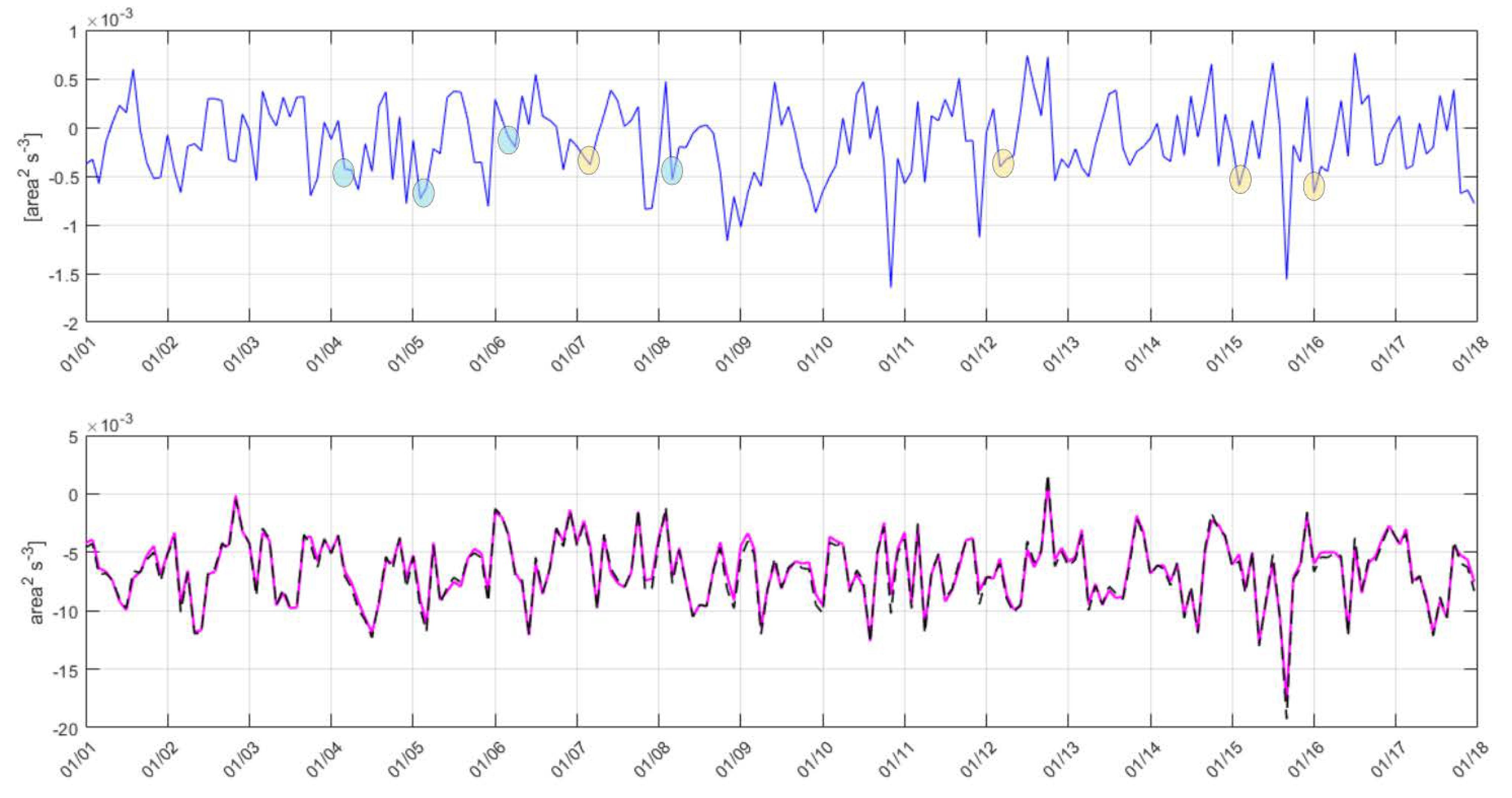
The intensity of the mixing and convection events depends mainly on the surface buoyancy fluxes B, which in turn depend on the heat fluxes through the air–sea interface, scaled by the thermal expansion coefficient α, and the freshwater fluxes, scaled by the haline contraction coefficient β. Monthly surface buoyancy fluxes and their thermal and haline (freshwater) components, integrated over the center of RG (longitude: 28–31°E, latitude: 34–36°N), are shown in Figure 4.
The haline components (BS) dominate the surface buoyancy fluxes (Figure4, Lower Panel), i.e., that intense evaporation, especially during the preconditioning phase (e.g., Figure 8 for winter 2006), controls the surface buoyancy loss. Detected events of pronounced (i.e., with a MLD deeper than 250 m) dense water formation by the Argo float data, are indicated with blue (RG) and yellow (coastline) circles (Table 1).
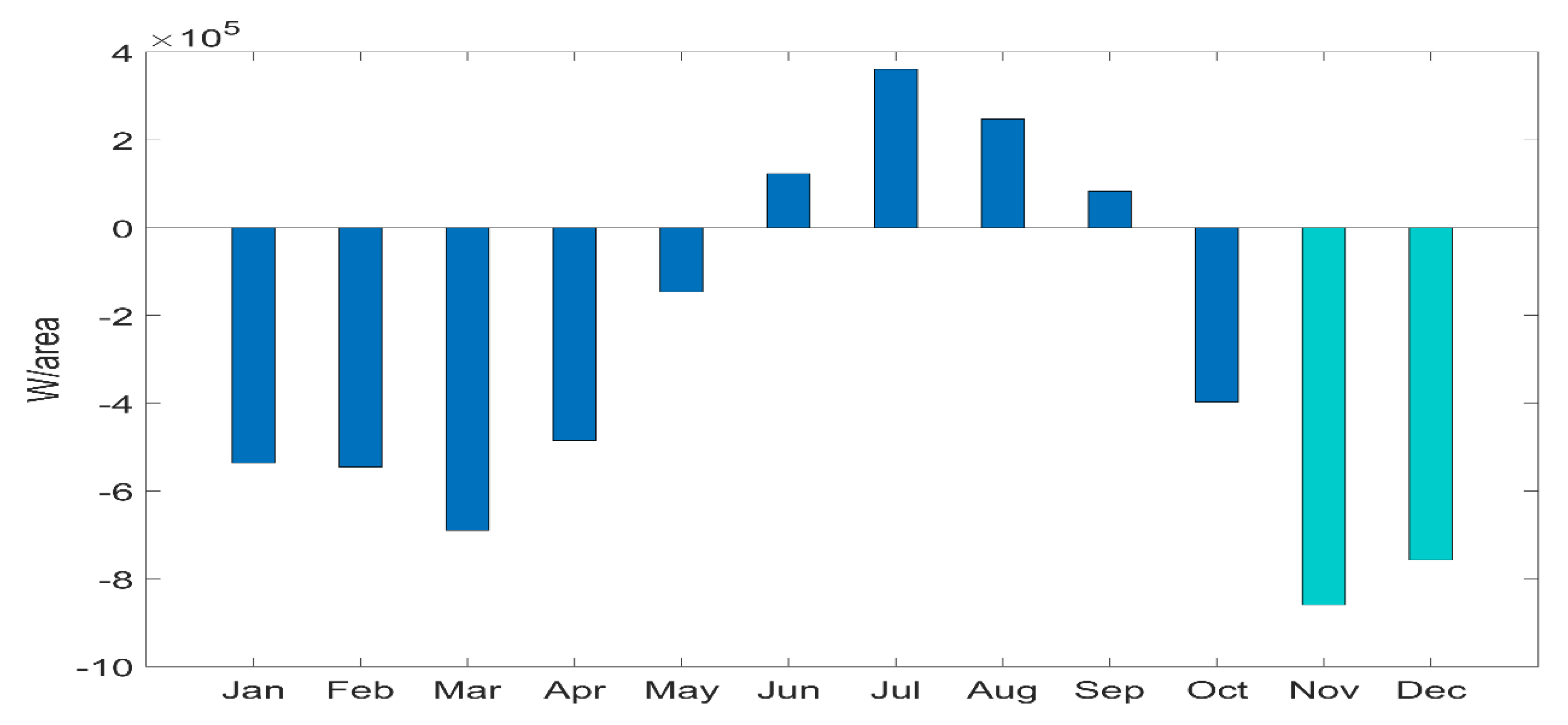
The climatology of monthly heat fluxes Qnet for the center of RG from 2001 to 2017 shows that the largest heat losses which induce the preconditioning phase occurred mainly in November and in December (Figure 5). The subsequent heat losses in JFM induce the formation of dense water and therefore lead to convection and mixing.
3.2. LIW and LDW Formation within the Northwestern Levantine Sea
Intermediate and deep water formation events in the NWLS (latitude: 33–37°N, longitude: 26–32°E) were analyzed during the winter months (JFM) from 2001 to 2017 (879 T/S profiles from 20 floats). Most of the float profiles within the NWLS showed ‘regular’ winter MLDs, i.e., MLDs between 100 and 200 m. Pronounced dense water formation, i.e., with a MLD deeper than 250 m, occurred only within the center of RG, along the Northern coastline and along the Cretan Arch passage. Events of pronounced LDW (13.7 °C < potential temperature < 14.5 °C, 38.8 psu < salinity < 38.9 psu) and ‘lower range’ LIW (potential temperature around 15 °C and salinity around 39 psu) formation were detected within the center of RG in winter 2004, 2005, 2006, and 2008 and events of pronounced LIW formation (potential temperature > 15 °C and salinity > 39 psu) were detected along the Northern coastline in winter 2007, 2012, 2015. and 2016 (Table 1). More than 800 profiles of 20 floats were analyzed, but only four floats (Table 1 and Table 2) captured pronounced dense water formation, being at the right place at the right time. To document the dense water formation events the float had to be either inside or pass later through the area of dense water formation. Float WMO 6900098 had an exceptionally long lifetime of nearly 6 years and therefore it was able to capture one event of pronounced LIW formation along the Northern coastline and four events of pronounced DWF. Unfortunately, it stopped measuring at 600 m depth. The WMO numbers of the Argo floats that found pronounced dense water formation events within the center of RG and along the coastline are listed in Table 2.
3.2.1. LDW formation within the Rhodes Gyre
Two examples of LDW formation within RG are given in this subsection.
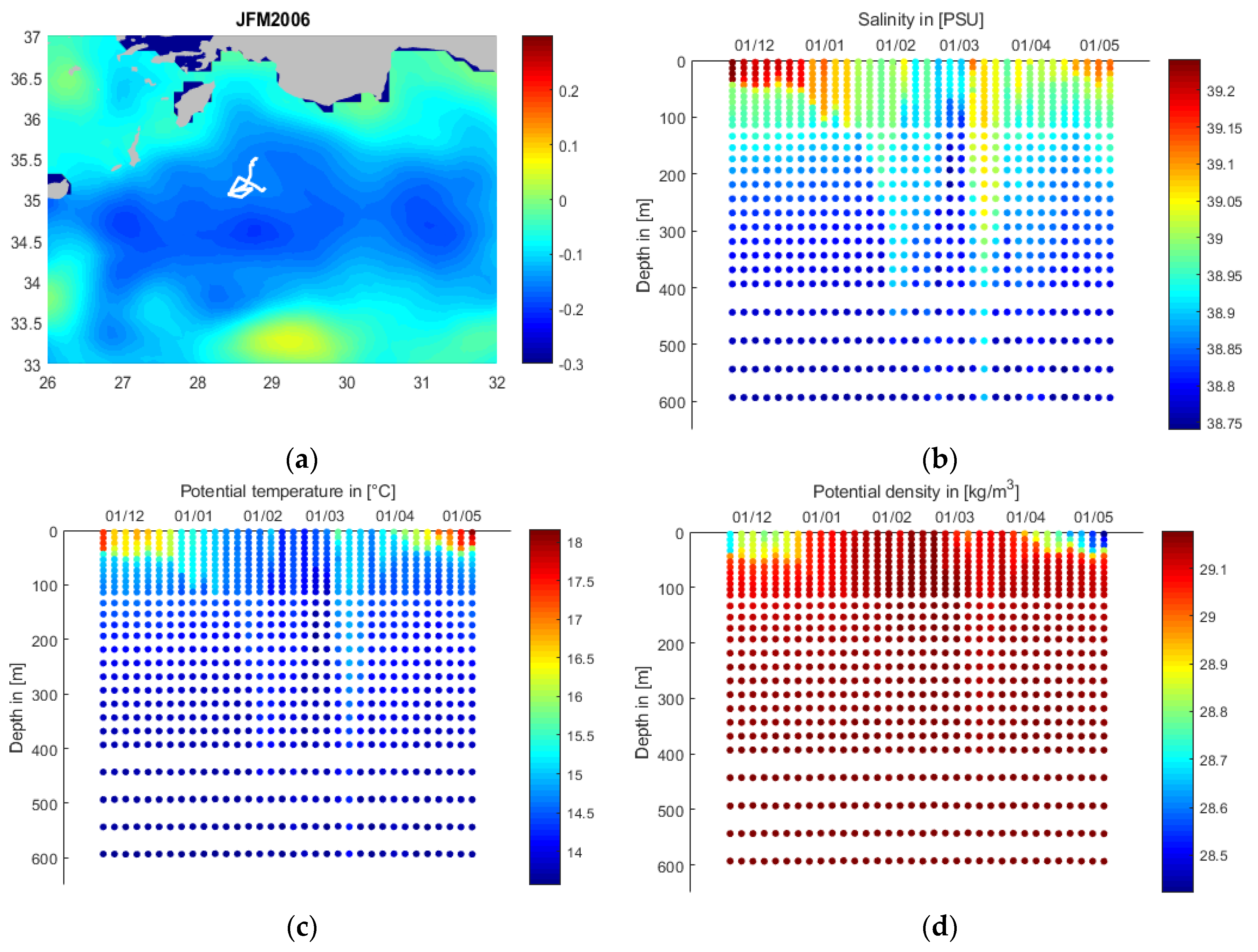
(1) In JFM 2006, float WMO 6900098 was entrapped in the center of RG (Figure 6a). Hoevmueller plots of salinity, potential temperature, and potential density describe two pronounced events of mixing and convection during this winter (Figure 6b–d). The first event occurred by the end of January until mid-February and led to LDW formation (13.7 °C < potential temperature < 14.5 °C, 38.8 psu < salinity < 38.9 psu) while the second event around mid-March led to LDW and ‘lower range’ LIW (temperature about 15°C and salinity about 39 psu) formation.
In December, very high surface salinity values (S > 39.15 psu) were detected in the upper 50 m (Figure 6b). However, mixing and convection is still prevented by relatively high surface temperatures during December. The surface temperature has a decreasing trend from 17.5 °C by the beginning of December to 15.5 °C in early January and reached a minimum of about 14 °C from the end of January to the end of February. From the beginning of March, the surface temperature gradually increased, reaching 15.5 °C during March with a successive increase to 17.5 °C by the end of April.
The MLD deepens from 50 m within December to about 100 m in the beginning of January and the high surface salinity is mixed to intermediate layers.
By the end of January, when lowest surface temperatures (T = 14–14.5 °C) are reached, dense water formation starts to occur. Potential density reaches its highest values (29.1 kg/m3) by the end of January until mid-February and the examination of single profiles shows that deep convection takes place down to at least 600 m during this period.
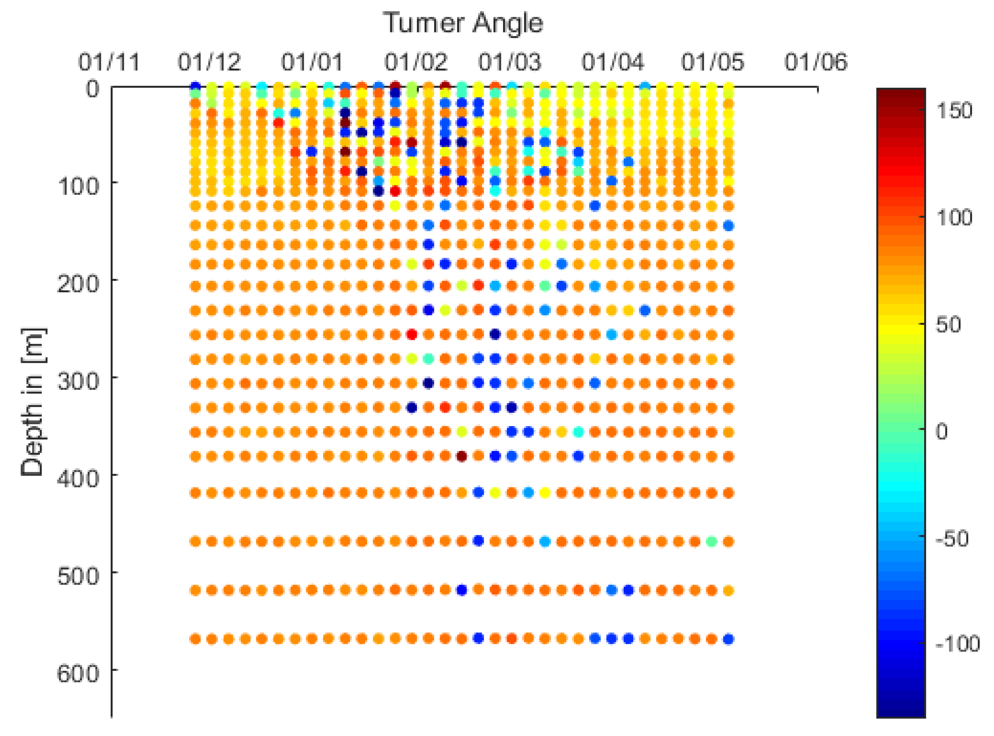
The Hoevmueller plot of the Turner angle (Figure 7) reveals statically unstable conditions (|Tu|> 90°; dark blue and dark red points) from mid-January to the end of March and indicates the deep dense water formation events down to at least 600 m in February and March 2006. The deep dense water formation events are characterized by a stronger contribution of temperature (−45° < Tu < −90°; blue points), while the main contributor to the stable stratification in December and April is mainly the salinity (45° < Tu < 90°; yellow and light orange points).
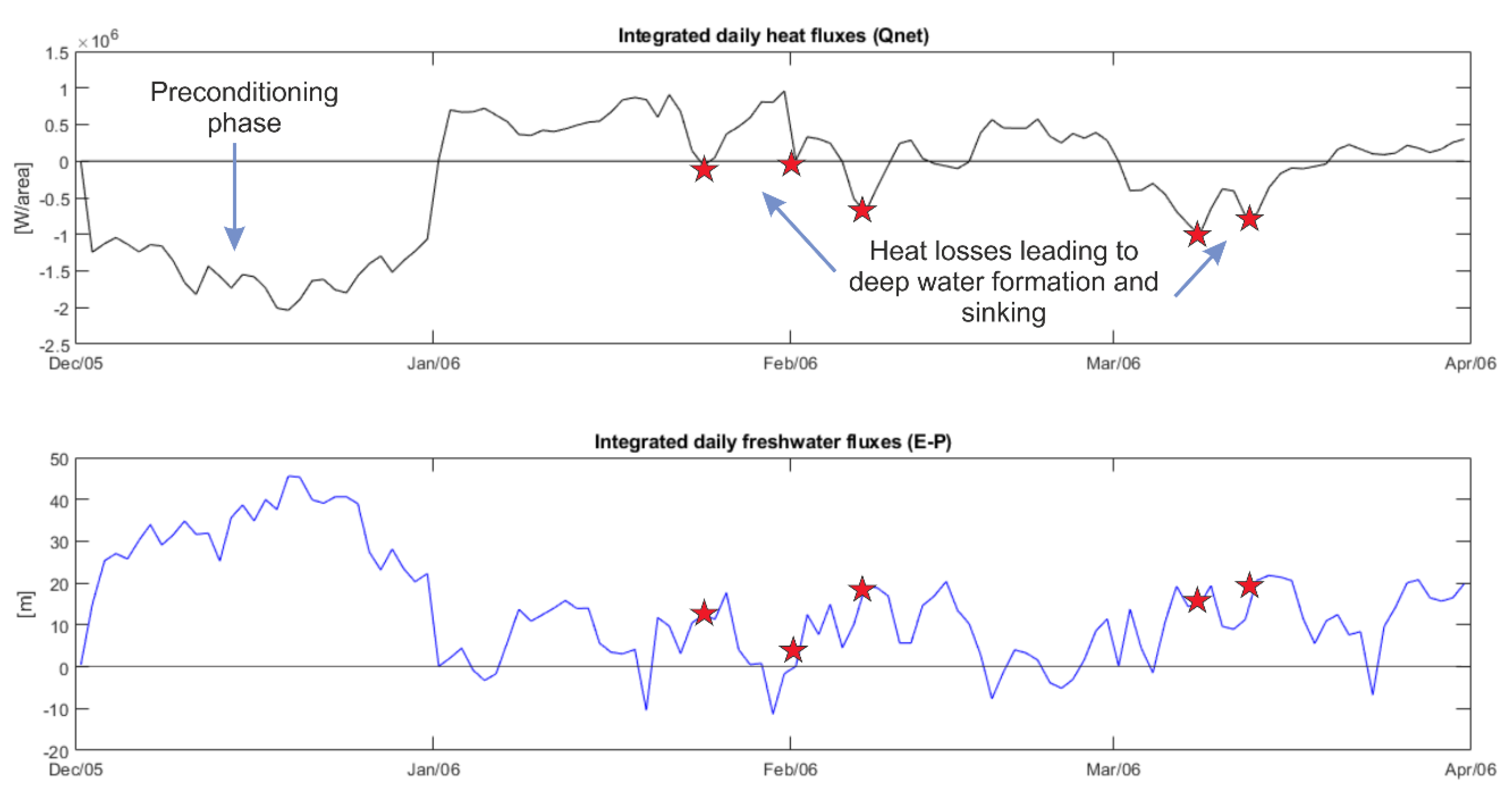
The heat and freshwater fluxes integrated over the center of RG show an intense preconditioning phase during December 2005, due to strong dry and cold winter winds which led to heat losses (Figure 8a) and evaporation (Figure 8b) and consequently to high surface salinity values. Additional heat losses by the end of January and the beginning of February coincide with the LDW formation event within the RG described above. The heat losses in mid-March coincide with the second dense water formation event within RG which led to a mixture of LDW and ‘lower range’ LIW formation.
This deep convection event from the end of January until mid-February coincides with a strong depression of SSH within the RG area during that time, overlapping the exact position of the float (longitude: 28.5–29°E, latitude: 35–35.5°N; Figure 9). Figure 9a shows the float trajectory and mean SSH of January, February, and March 2006 while Figure 9b,c,d show the negative daily SSH and geostrophic currents for three specific days during the period of deep convection event from the end of January to mid-February. The eddy in which the float was trapped, represents the strongest depression (SSH < −0.3 m; about 20 cm below the seasonal mean (Figure 9a)) during winter months reaching a negative maximum during the days of deep water formation (Figure 6b–d).
The mesoscale eddy during that time shows a diameter of about 60 km which is within the typical mesoscale eddy diameter within the Levantine Sea (40–80 km).
Figure 10 shows the monthly means of satellite SST superimposed on the geostrophic currents derived from SSH. The deep convection event occurred by the end of January until mid-February 2006 when the sea surface temperature was lowest. The lowest surface temperatures measured by the Argo float, evidenced within the Hoevmueller plots (Figure 6c), coincide with lowest temperatures by daily satellite SST (Figure 10e,f) and with the strongest depression of SSH (Figure 9b–d) by the end of January until mid-February.
Figure 11 shows the T/S plots for the two events of dense water formation during JFM 2006. Water masses above 100 m were not taken into account for the T/S plot to exclude shallow MLDs and recapping and to capture the events of pronounced intermediate and deep water formation. Water masses from 100 to 500 m are plotted with a green dot while water masses under 500 m are plotted with blue dots.
Figure 11a shows the T/S plot for the first dense water formation event: The potential temperature exhibits values smaller than 14.5 °C, the salinity shows values smaller than 39 psu, and the potential density shows a constant value of about 29.17 kg/m3. The typical ranges for LDW for potential temperature are between 13.7 °C and 14.5 °C and for salinity between 38.8 to 38.9 psu [6,9,10]. The potential density line of 29.17 kgm−3 represents the upper deep-water boundary density for the NWLS, corresponding to approximately 1000 m depth [23]. All potential temperatures and salinity values lay on the line of constant potential density of 29.17 kgm−3, i.e., that the formed water masses sank to at least 1000 m, until the same potential density was reached. Therefore, the T/S plot confirms that LDW took place during the first event by late January until mid-February (Figure 11a).
For the dense water formation event in March 2006, the T/S plot shows potential temperatures smaller than 15 °C, salinities smaller than 39.1 psu, and potential densities between 29.125 kg/m3 and 29.17 kg/m3. By nearly reaching 15 °C and with some salinity values above 39 psu, a part of the water mass reaches the lower range of LIW water mass characteristics (Figure 11b). This indicates a mixture of LDW and ‘lower range’ LIW formation during the second dense water formation event within RG.
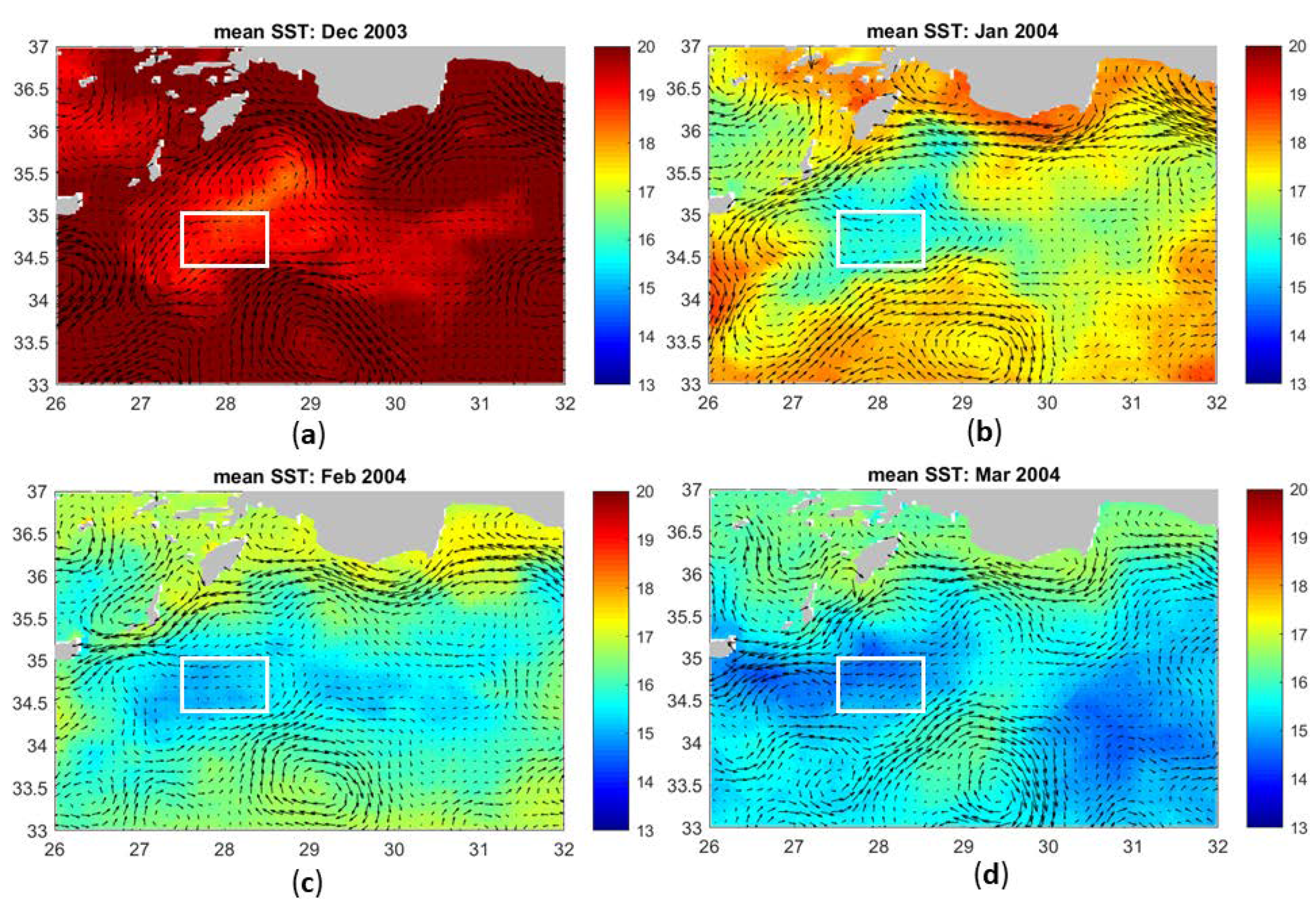
(2) LDW formation took also place from the end of February until mid-March 2004 within another cyclonic mesoscale eddy located in the western part of the RG. Hoevmueller plots for DJFMA for salinity, potential temperature, and potential density are shown in Figure 12. During January and February, the MLD deepens constantly and the event of LDW formation occurs by the end of February until mid of March when the minimum surface temperature was reached. The examination of single profiles shows convection down to at least 600 m.
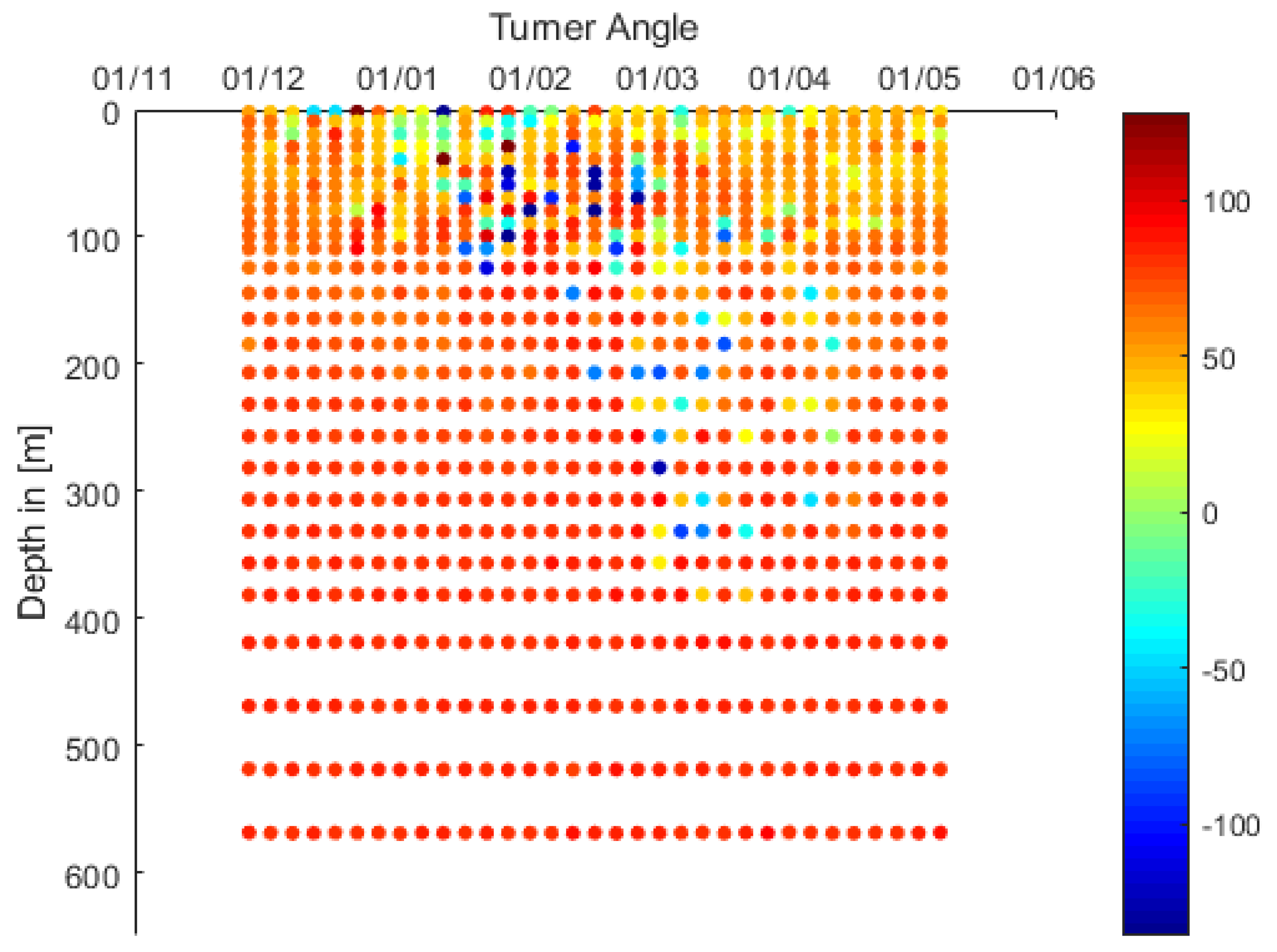
The Hoevmueller plot of the Turner angle (Figure 13) reveals statically unstable conditions (|Tu| > 90°; dark blue and dark red points) and therefore a continuous deepening of the MLD from mid-January to mid-March 2004 and indicates the deep dense water formation events down to 400 m by the end of February and mid-March. The main contributor to the stable stratification in December and April is the salinity (45° < Tu < 90°; yellow and light orange points), while the deep dense water formation events are also characterized by a stronger contribution of temperature gradients (−45° < Tu < −90°; blue points). ‘Salt-fingering’ (45° < Tu < 90°; yellow points) can be noticed at a depth of about 350 m.
The T/S plot of JFM2004 shows mainly LDW formation (Figure 14). Green dots represent water masses between 100 and 500 m while blue dots represent water masses between 500 and 600 m. The water mass characteristics show LDW and ‘lower range’ LIW (potential temperature around 15 °C and 39 psu < salinity < 39.1 psu) formation.
Figure 15 shows: (a) the mean SSH for JFM 2004 and the float trajectory (longitude: 27.5°E–28.5°E, latitude: 34.5°N–35°N) during this period and daily SSH (b) before; (c) during; and (d) after the convection event. A strong powerful structure develops by mid-February with a negative SSH of more than −0.3 m. Analysis of single profiles shows that on 8 March 2004, a MLD down to about 450 m was formed while on the surface recapping already took place (newly formed MLD of about 80 m).
3.2.2. LIW Formation along the Coastline
One example of LIW formation along the coastline is given in this subsection.
While LDW was formed inside RG, typical LIW was instead formed along the Northern Turkish coastline, i.e., along the AMC. The salinity, potential temperature, and potential density values characterize a typical LIW formation event by the end of March (Figure 17).
In December and January, very high surface salinity values (S > 39.3 psu) can be seen in the upper 50 to 100 m (Figure 17b). However, deep mixing and convection is still prevented by relatively high surface temperatures (T > 17 °C) during this period. Surface temperature has a decreasing trend from about 20 °C by the very beginning of December to about 17 °C in March when deep convection occurs. By the end of April, the surface temperature gradually increases reaching 17.5 °C. The observed surface water temperature along the coastline is about 1 °C to 3 °C warmer than in the open sea (Figure 6 and Figure 12).
The MLD deepens gradually from about 50 m within December to about 250 m during February; therefore, the high surface salinity is mixed throughout intermediate layers (Figure 17b).
By the end of March, when lowest surface temperatures are reached (Figure 17c), dense water formation starts to occur. Surface potential density reaches values between 29 and 29.1 kg/m3 during this period. The examination of single profiles shows that the mixing event takes place down to about 550 m.
The Hoevmueller plot of the Turner angle (Figure 18) reveals statically unstable conditions (|Tu|> 90°; dark blue and dark red points) and therefore a continuous deepening of the MLD in January and February 2007. The main contributors to the stratification in December are both temperature and salinity (−45° < Tu < 45°), while in April the main contributor is the salinity (45° < Tu < 90°; yellow and light orange points). The Turner angle indicates the deep LIW formation event down to 550 m in March, which is also characterized by a stronger contribution of temperature gradients (−45° < Tu < −90°; blue points).
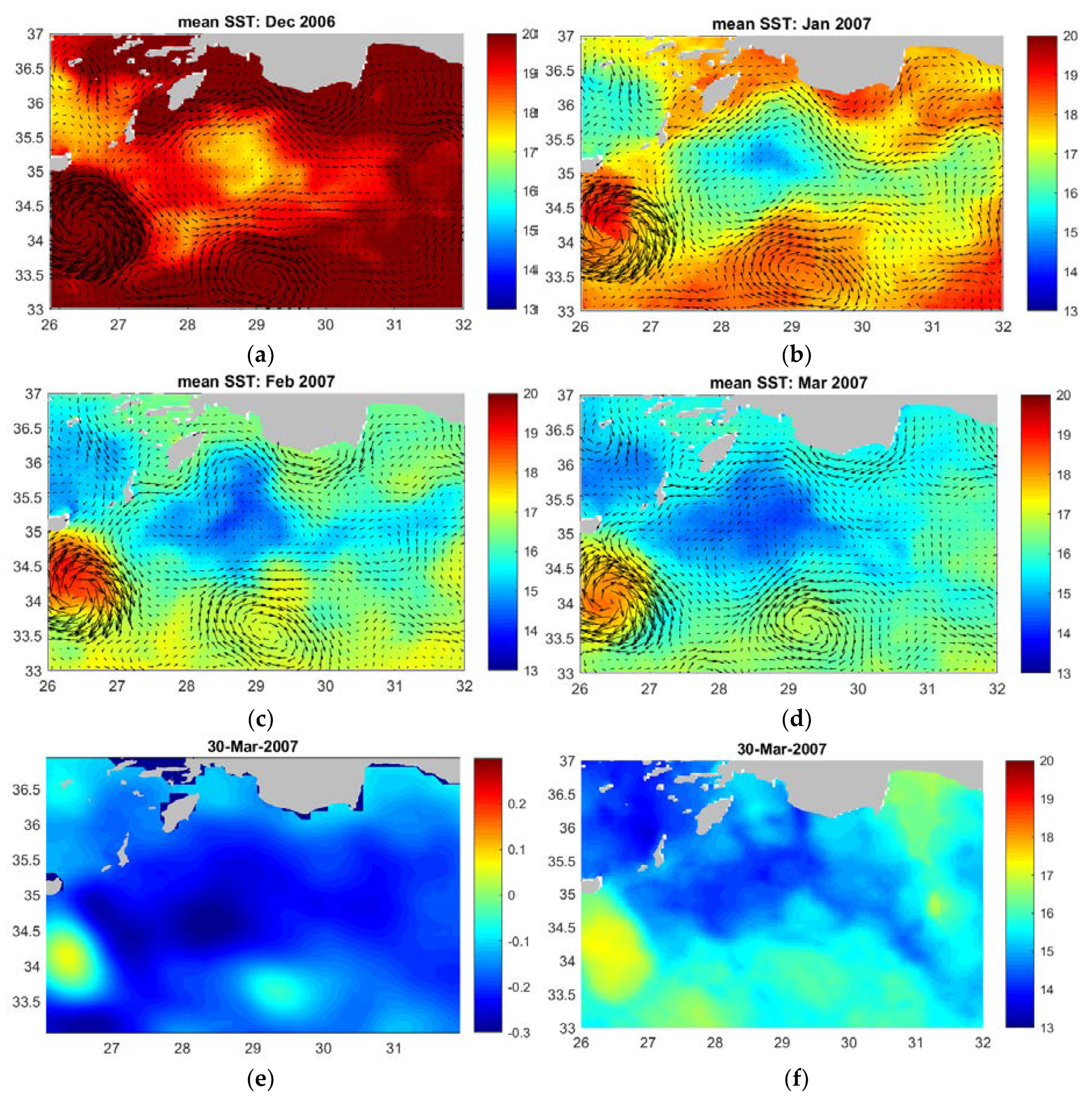
The evolution of monthly mean SST from December 2007 to March 2007 is shown in Figure 19a–d. This deep convection event that was detected by the Argo float by the end of March 2007 coincides with the strongest depression of SSH and lowest surface temperatures along the coastline during winter 2007 (Figure 19a–c).
3.3. Climatology of Winter Mean MLD from 2000 to 2018
The climatology of the winter (JFM) mean MLD from 2000 to 2018 for the Levantine Sea is shown in Figure 21. Within the cyclonic RG, the mean winter MLD is quite shallow (around 70 m). Deeper mean winter MLDs are found within anticyclonic eddies (IE, MME, CE, ShE; see Figure 1b for position of eddies) and along the coastlines, indicating dense water formation along boundary currents.
4. Discussion and Conclusions
The present study is focused on the LIW and LDW formation events in the NWLS (Figure 22a) as detected by Argo float data from 2001 to 2017. The new and most interesting result is that the typical LIW (potential temperature > 15 °C and salinity > 39 psu) formation mainly occurred along the Northern coastline (Figure 18), while ‘lower range’ LIW (potential temperature about 15 °C and salinity about 39 psu) and LDW (13.7 °C < potential temperature < 14.5 °C, 38.8 psu < salinity < 38.9 psu) formation took place within mesoscale eddies located within the center of RG (Figure 22a; Figure 11a, Table 1).
The schematic summary of the results for the winter seasons from 2001 to 2017 is evident in Figure 22b. Blue and brown arrows describe the convection and net sinking areas of the Mediterranean Sea as derived from theoretical models by [15,16]. Red and orange arrows are derived from the results of the present work. Red solid and dashed lines represent the formation of intermediate (200–500 m) and deeper waters (500–600 m) along the Northern coastline. Orange arrows represent the formation of intermediate (200–500 m) and deep waters (about 1000 m) within the RG, respectively. The examination of individual profiles showed dense water formation events reaching down to 550 m depth along the coastline and down to 1000 m depth within the center of RG (Figure 22b).
The specific event of LIW formation, captured by the Argo float data in March 2007 along the coastline, reached a depth of about 550 m. The T/S plot (Figure 20) showed typical LIW formation during this event and the observed surface water temperature along the coastline was about 1°C to 3°C warmer than in the open sea (Figure 6, Figure 12 and Figure 17), in agreement with the results of [24,25]. In January–February 2006, the Argo float data detected the LDW formation in the core of a cyclonic mesoscale structure located in the center of RG. This structure (diameter of about 60 km) shows the typical horizontal scale of convective chimneys. The T/S plot in Figure 11a reveals the LDW characteristics of the convection event. All potential temperatures and salinity values lay on the line of constant potential density of 29.17 kgm−3, revealing the sinking of the formed water masses to at least 1000 m as previously observed [6,9,10].
The intensity of the mixing and convection events depends mainly on the surface buoyancy flux B, which in turn depends on its thermal (BT) and haline (BS) components. The calculation and plot of the surface buoyancy flux and its components revealed that the haline component dominates over the thermal component (Figure 4, lower panel), i.e., intense evaporation (BS < 0) controls the surface buoyancy loss, especially during the preconditioning phase (e.g., Figure 8 for winter 2006). Therefore, the area of the RG is an area of net buoyancy loss, driven by the haline component, as shown by [26].
The influence of salinity and temperature gradients to the density gradients are described in the Hoevmueller diagrams of the Turner angle (Figure 7, Figure 13 and Figure 18). During the preconditioning phase (November, December) and the constant deepening of the MLD in the beginning of January, the influence of the salinity gradient was dominant, while during strong unstable conditions and consequently dense water formation, also the temperature gradient was influential. The Turner angle also approximately indicated the depth of the convection events.
The deep dense water formation events within the area of the RG can be described by the following phases: The whole process is influenced by the cyclonic rotation of the RG leading to the upwelling of cooler waters to the surface. In November and December, the preconditioning phase starts (Figure 4 and Figure 5): the heat losses due to cold and dry winds lead to increased surface salinity (Figure 6, Figure 12 and Figure 17) through the evaporation and to a steady deepening of the MLD. Additional, temporarily outbreaks of strong winds during January, February, or March cause strong heat losses (Figure 5 and Figure 8), which cause further cooling of surface waters. When lowest surface temperatures are reached (Figure 10, Figure 16 and Figure 19), dense water formation starts to occur. Within hours, the newly formed dense water sinks down rapidly to a depth of equal density where it spreads horizontally, forming an anticyclonic circulation due to the influence of the Coriolis force.The convection event also implicates a stretching of the water column leading to a change in vorticity, an increased geostrophic velocity, and a depression of the SSH. In fact, all pronounced dense water formation events documented by the Argo floats were indicated by a strong depression of satellite SSH (Figure 9, Figure 15 and Figure 19) and by lowest SSTs (Figure 10, Figure 16 and Figure 19).
The Argo float data revealed that LDW formation took place within the RG during winter months and showed the key role of the boundary currents for the LIW formation. The climatology of the mean MLDs of the Levantine Sea (Figure 21) reveals that, despite the deep convection events, little to net mean sinking takes place within the center of RG, while the deeper MLDs along the coastline indicate dense water formation occurring along boundary currents. Therefore, the drivers, sources, and main contributors of the Mediterranean thermohaline circulation have to be rethought not only within the Levantine, but also within the Mediterranean Sea. Deployments of additional Argo floats to survey boundary currents and deployment of deep Argo floats within the main Mediterranean convection sites, i.e., the Gulf of Lion, the South Adriatic, and the RG area, will contribute to further understanding of dense water formation processes.
A better understanding of the Mediterranean thermohaline circulation is needed not only for a wider knowledge of the effects of climate change, but also for the impact on the ecology. Newly formed intermediate or deep waters can be polluted (with oil, microplastics, nutrients from extensive agriculture, heat due to global warming etc.), e.g., the Northern Levantine coastline, where pronounced dense water formation occurs, has the highest coastline plastic pollution within the Mediterranean Sea [27]. The newly formed water masses with the above-mentioned water properties and pollutants are transported throughout the Mediterranean to finally reach the Atlantic Ocean. The full impact (in terms of pollution and different water mass characteristics) will only be seen by future generations when these water masses emerge after decades or even centuries at different places within the Mediterranean Sea.
Therefore, it is obvious and evident that scientists and policy makers are obliged to join forces now to support and make commitments towards a real sustainable world that is not threatening, but protecting our ecosystems and lives.
Author Contributions
Conceptualization, E.K., P.-M.P. and E.M.; methodology, E.K., G.N. and M.M.; writing—original draft preparation, E.K.; writing—review and editing, M.M., E.M., P.-M.P. and G.N.; investigation, E.K.; data curation, E.K. and G.N.; supervision, P.-M.P. and E.M.; funding acquisition, P.-M.P.
Funding
The float data were collected and made freely available by the International Argo Program and the national programs that contribute to it (http://argo.jcommops.org). The Argo Program is part of the Global Ocean Observing System.
Acknowledgments
The authors would like to thank the two anonymous reviewers for their constructive comments and all the people who have deployed Argo floats in the Mediterranean Sea. We acknowledge Antonio Bussani and Massimo Pacciaroni for their technical support with the dataset and floats programming. In addition, we thank Vedrana Kovacevic for her suggestions and fruitful discussions.
Conflicts of Interest
The authors declare no conflict of interest.
References
- Tsimplis, M.N.; Zervakis, V.; Josey, S.A.; Peneva, E.L.; Struglia, M.V.; Stanev, E.V.; Theocharis, A.; Lionello, P.; Malanotte-Rizzoli, P.; Artale, V.; et al. Changes in the Oceanography of the Mediterranean Sea and their Link to Climate Variability, in Mediterranean Climate Variability. In Developments in Earth & Environmental Sciences; Lionello, P., Malanotte-Rizzoli, P., Boscolo, R., Eds.; Elsevier: Amsterdam, The Netherlands, 2006; Volume 4, pp. 227–282. [Google Scholar]
- Bergamasco, A.; Malanotte-Rizzoli, P. The circulation of the Mediterranean Sea: A historical review of experimental investigations. Adv. Oceanogr. Limnol. 2010, 1, 11–28. [Google Scholar] [CrossRef]
- Gacic, M.; Civitarese, G.; Eusebi Borzelli, G.L.; Kovacevic, V.; Poulain, P.-M.; Theocharis, A.; Menna, M.; Catucci, A.; Zarokanellos, N. On the relationship between the decadal oscillations of the Northern Ionian Sea and the salinity distributions in the Eastern Mediterranean. J. Geophys. Res. (Ocean.) 2011, 116. [Google Scholar] [CrossRef]
- Gacic, M.; Schroeder, K.; Civitarese, G.; Vetrano, A.; Eusebi Borzelli, G.L. On the relationship among the Adriatic-Ionian Bimodal Oscillating System (BiOS), the Eastern Mediterranean salinity variations and the Western Mediterranean thermohaline cell. Ocean Sci. Discuss. 2012, 9, 2561–2580. [Google Scholar] [CrossRef]
- Menna, M.; Suarez, C.; Civitarese, G.; Gacic, M.; Poulain, P.-M.; Rubino, A. Decadal variations of circulation in the Central Mediterranean and its interactions with mesoscale gyres. Deep Sea Res. Part II Top. Stud. Oceanogr. 2019. [Google Scholar] [CrossRef]
- Malanotte-Rizzoli, P.; Manca, B.; Marullo, S.; Ribera d’Alcala, M.; Roether, W.; Theocharis, A.; Bergamasco, A.; Budillon, G.; Sansone, E.; Civitarese, G.; et al. The Levantine Intermediate Water Experiment (LIWEX) Group: Levantine basin—A laboratory for multiple water mass formation processes. J. Geophys. Res. 2003, 108, 8101. [Google Scholar] [CrossRef]
- Theocharis, A.; Krokos, G.; Velaoras, D.; Korres, G. An Internal Mechanism Driving the Alternation of the Eastern Mediterranean Dense/DeepWater Sources. The Mediterranean Sea: Temporal Variability and Spatial Patterns. In The Mediterranean Sea: Temporal Variability and Spatial Patterns, 1st ed.; Eusebi Borzelli, G.L., Gagic, M., Lionello, P., Malanotte-Rizzoli, P., American Geophysical Union, Eds.; Geophysical Monograph 202; John Wiley & Sons: Hoboken, NJ, USA, 2014; Volume 10, pp. 113–137. [Google Scholar]
- Lionello, P.; Malanotte-Rizzoli, P.; Boscolo, R.; Alpert, P.; Artale, V.; Li, L.; Luterbacher, J.; May, W.; Trigo, R.; Tsimplis, M.; et al. The Mediterranean Climate: An Overview of the Main Characteristics and Issues. Dev. Earth Environ. Sci. 2006, 4, 1–26. [Google Scholar]
- Sur, H.I.; Özsoy, E.; Unluata, U. Simultaneous deep and intermediate depth convection in the Northern Levantine Sea, winter 1992. Oceanol. Acta 1993, 16, 33–43. [Google Scholar]
- Gertman, I.F.; Ovchinnikov, I.M.; Popov, Y.I. Deep convection in the eastern basin of the Medi-terranean Sea. Oceanology 1994, 34, 19–25. [Google Scholar]
- Spall, M.A.; Pickart, R.S. Where does dense water sink? A subpolar gyre example. J. Phys. Oceanogr. 2001, 31, 810–826. [Google Scholar] [CrossRef]
- Spall, M.A. Boundary currents and water mass transformation in marginal seas. J. Phys. Oceanogr. 2004, 34, 1197–1213. [Google Scholar] [CrossRef]
- Spall, M.A. Buoyancy-forced downwelling in boundary currents. J. Phys. Oceanogr. 2008, 38, 2704–2721. [Google Scholar] [CrossRef]
- Spall, M.A. Dynamics of downwelling in an eddy-resolving convective basin. J. Phys. Oceanogr. 2010, 40, 2341–2347. [Google Scholar] [CrossRef]
- Waldman, R.; Brüggemann, N.; Bosse, A.; Spall, M.; Somot, S.; Sevault, F. Overturning the Mediterranean Thermohaline Circulation. Geophys. Res. Lett. 2018. [Google Scholar] [CrossRef]
- Pinardi, N.; Cessi, P.; Borile, F.; Wolfe, C. The Mediterranean Sea Overturning Circulation. J. Phys. Oceanogr. 2019. [Google Scholar] [CrossRef]
- Menna, M.; Poulain, P.-M.; Zodiatis, G.; Gertman, I. On the surface circulation of the Levantine sub-basin derived from Lagrangian drifters and satellite altimetry data. Deep Sea Res. Part I Oceanogr. Res. Pap. 2012, 65, 46–58. [Google Scholar] [CrossRef]
- Poulain, P.-M.; Barbanti, R.; Font, J.; Cruzado, A.; Millot, C.; Gertman, I.; Griffa, A.; Molcard, A.; Rupolo, V.; Le Bras, S.; et al. MedArgo: A drifting profiler program in the Mediterranean Sea. Ocean Sci. 2007, 3, 379–395. [Google Scholar] [CrossRef]
- Holte, J.; Talley, L.D.; Gilson, J.; Roemmich, D. An Argo mixed layer climatology and database. Geophys. Res. Lett. 2017, 44, 5618–5626. [Google Scholar] [CrossRef] [Green Version]
- Zahariev, K.; Garrett, C. An Apparent Surface Buoyancy Flux Associated with the Nonlinearity of the Equation of State. J. Phys. Oceanogr. 1997, 27, 362–368. [Google Scholar] [CrossRef]
- Ruddick, B.R. A practical indicator of the stability of the water column to double-diffusivity activity. Deep Sea Res. Part A 1983, 30, 1105–1107. [Google Scholar] [CrossRef]
- IOC; SCOR; IAPSO. The International Thermodynamic Equation of Seawater—2010: Calculation and Use of Thermodynamic Properties; Intergovernmental Oceanographic Commission, UNESCO (English): Paris, France, 2010; p. 196. [Google Scholar]
- Roether, W.; Klein, B.; Manca, B.B.; Theocharis, A.; Kioroglou, S. Transient Eastern Mediterranean deep waters in response to the massive dense-water output of the Aegean Sea in the 1990’s. Prog. Oceanogr. 2007, 74, 540–571. [Google Scholar] [CrossRef]
- Feliks, Y. Downwelling along the Northeastern Coasts of the Eastern Mediterranean. J. Phys. Oceanogr. 1991, 21, 511–526. [Google Scholar] [CrossRef] [Green Version]
- Feliks, Y.; Ghil, M. Downwelling-front instability and eddy formation in the Eastern Mediterranean. J. Phys. Oceanogr. 1993, 23, 61–78. [Google Scholar] [CrossRef]
- Karstensen, J.; Lorbacher, K. A practical indicator for surface ocean heat and freshwater buoyancy fluxes and its application to the NCEP reanalysis data. Tellus 2011, 63, 338–347. [Google Scholar] [CrossRef] [Green Version]
- WWF Mediterranean Marine Initiative Report. Stop the Flood of Plastic: How Mediterranean Countries Can Save Their Sea. 2019. Available online: http://awsassets.panda.org/downloads/a4_plastics_reg_low.pdf (accessed on 25 June 2019).
Figure 1.
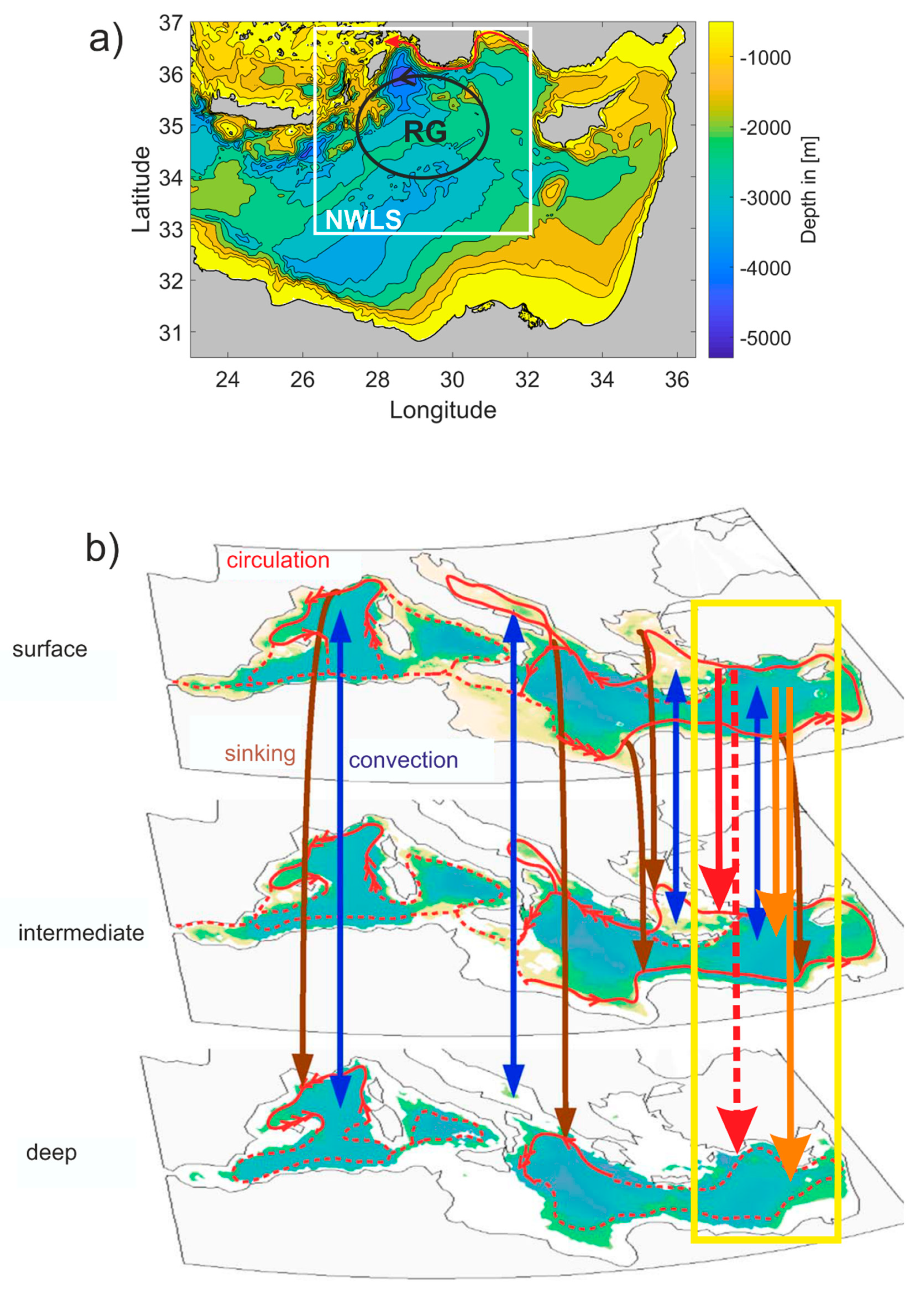
(a) General concept of the thermohaline circulation which, according to the prevailing view, is driven by a few convection sites within the Mediterranean Sea, adapted from [1]. The red arrow shows the entering Atlantic water (AW) while the orange arrow shows the Levantine intermediate water (LIW), which travels throughout the Mediterranean and flows into the Atlantic Ocean. The orange and yellow frames highlight the area of the Levantine Sea and of the Northwestern Levantine Sea (NWLS), respectively. The blue circle indicates the position of the North Ionian Gyre (NIG) the circulation of which is important for the advective salinity preconditioning. (b) Mean surface geostrophic circulation in the Levantine Sea from 1992 to 2010 derived from drifter data. The yellow rectangle indicates the area of study, the NWLS (latitude: 33–37°, longitude: 26–32°). Adapted from [17]. AMC—Asia Minor Current; CC—Cilician Current; CE—Cyprus Eddy; EE—Egyptian Eddies; IE—Ierapetra Eddy; LEC—Libyo-Egyptian Current; LTE—Latakia Eddy; MME—Mersa-Matruh Eddy; MMJ—Mid Mediterranean Jet; ShE—Shikmona Eddy. (c) A model run from 1980 to 2013 [15] showed that little to no net sinking takes place at convection sites (blue arrows; from left to right: Gulf of Lion, South Adriatic, Aegean Sea, Rhodes Gyre (RG)) while boundary layer currents undergo net intense sinking (brown arrows). The yellow rectangle indicates the area of study. Adapted from [15].
Figure 1.
(a) General concept of the thermohaline circulation which, according to the prevailing view, is driven by a few convection sites within the Mediterranean Sea, adapted from [1]. The red arrow shows the entering Atlantic water (AW) while the orange arrow shows the Levantine intermediate water (LIW), which travels throughout the Mediterranean and flows into the Atlantic Ocean. The orange and yellow frames highlight the area of the Levantine Sea and of the Northwestern Levantine Sea (NWLS), respectively. The blue circle indicates the position of the North Ionian Gyre (NIG) the circulation of which is important for the advective salinity preconditioning. (b) Mean surface geostrophic circulation in the Levantine Sea from 1992 to 2010 derived from drifter data. The yellow rectangle indicates the area of study, the NWLS (latitude: 33–37°, longitude: 26–32°). Adapted from [17]. AMC—Asia Minor Current; CC—Cilician Current; CE—Cyprus Eddy; EE—Egyptian Eddies; IE—Ierapetra Eddy; LEC—Libyo-Egyptian Current; LTE—Latakia Eddy; MME—Mersa-Matruh Eddy; MMJ—Mid Mediterranean Jet; ShE—Shikmona Eddy. (c) A model run from 1980 to 2013 [15] showed that little to no net sinking takes place at convection sites (blue arrows; from left to right: Gulf of Lion, South Adriatic, Aegean Sea, Rhodes Gyre (RG)) while boundary layer currents undergo net intense sinking (brown arrows). The yellow rectangle indicates the area of study. Adapted from [15].

Figure 2.
(a) Position of the 879 analyzed float profiles for January, February, and March (JFM) 2001–2017; Orange rectangle defines the area of study (the NWLS), the black ellipse describes the center of RG. (b) Annual distribution of float profiles in the NWLS: JFM 2001–2017.
Figure 2.
(a) Position of the 879 analyzed float profiles for January, February, and March (JFM) 2001–2017; Orange rectangle defines the area of study (the NWLS), the black ellipse describes the center of RG. (b) Annual distribution of float profiles in the NWLS: JFM 2001–2017.

Figure 3.
(a) Climatology of the winter maximum mixed layer depth (colors) and location of float profiles (grey dots) from 2000 to 2018. The white rectangle indicates the area of study, the NWLS. (b) Trajectory of the float WMO 6900098 during JFM 2007; the numbers along the trajectory show the locations of float profiles. Float potential density profiles at cycle 2 (c), 5 (d), and 13 (e).

Figure 4.
Upper panel: Time series of the monthly thermal component (BT) from 2001 to 2017, integrated over the center of RG (longitude: 28–31°E, latitude: 34–36°N). Blue and yellow circles indicate events of pronounced dense water formation detected by the Argo floats within RG and along the coastline, respectively (Table 1). Lower panel: Time series of the monthly haline component (BS; magenta line) and buoyancy fluxes (B; black dotted line).

Figure 5.
Climatology of monthly integrated heat fluxes for the center of RG from 2001 to 2017. Main heat losses generally occur in November and December (turquoise bars) and initiate the preconditioning phase. Subsequent heat losses in January, February, and March induce dense water formation.
Figure 5.
Climatology of monthly integrated heat fluxes for the center of RG from 2001 to 2017. Main heat losses generally occur in November and December (turquoise bars) and initiate the preconditioning phase. Subsequent heat losses in January, February, and March induce dense water formation.

Figure 6.
(a) Mean sea surface height (SSH, m) and float trajectory of float WMO 6900098 for JFM 2006. (b) Salinity (PSU), (c) potential temperature (°C) and (d) potential density (kg/m3) from December 2005 to April 2006.
Figure 6.
(a) Mean sea surface height (SSH, m) and float trajectory of float WMO 6900098 for JFM 2006. (b) Salinity (PSU), (c) potential temperature (°C) and (d) potential density (kg/m3) from December 2005 to April 2006.

Figure 7.
The Turner angle (°) of float WMO 6900098 describes the contribution of salinity and temperature gradients to the density gradient.
Figure 7.
The Turner angle (°) of float WMO 6900098 describes the contribution of salinity and temperature gradients to the density gradient.

Figure 8.
Upper panel: Time series of integrated daily surface heat fluxes from December 2005 to April 2006 for the center of Rhodes Gyre. The heat losses by the end of January and mid-February induced deep convection and formation of Levantine deep water (LDW) while the heat losses in March induced mixing and formation of LDW and ‘lower range’ LIW (see also Figure 6). Lower panel: Time series of integrated daily freshwater fluxes for the same time period as the above panel. The freshwater fluxes in December show a strong evaporation which led to increased surface salinity as shown by the Argo float data (Figure 6b).

Figure 9.
(a) Trajectory of float WMO 6900098 depicted within white rectangle overlaid on mean SSH (m) for JFM 2006 for the NWLS. (b–d) daily SSH (m) during the LDW convection events (from 25 January to 7 February 2006). The mesoscale eddy within the white box has a diameter of about 60 km.
Figure 9.
(a) Trajectory of float WMO 6900098 depicted within white rectangle overlaid on mean SSH (m) for JFM 2006 for the NWLS. (b–d) daily SSH (m) during the LDW convection events (from 25 January to 7 February 2006). The mesoscale eddy within the white box has a diameter of about 60 km.

Figure 10.
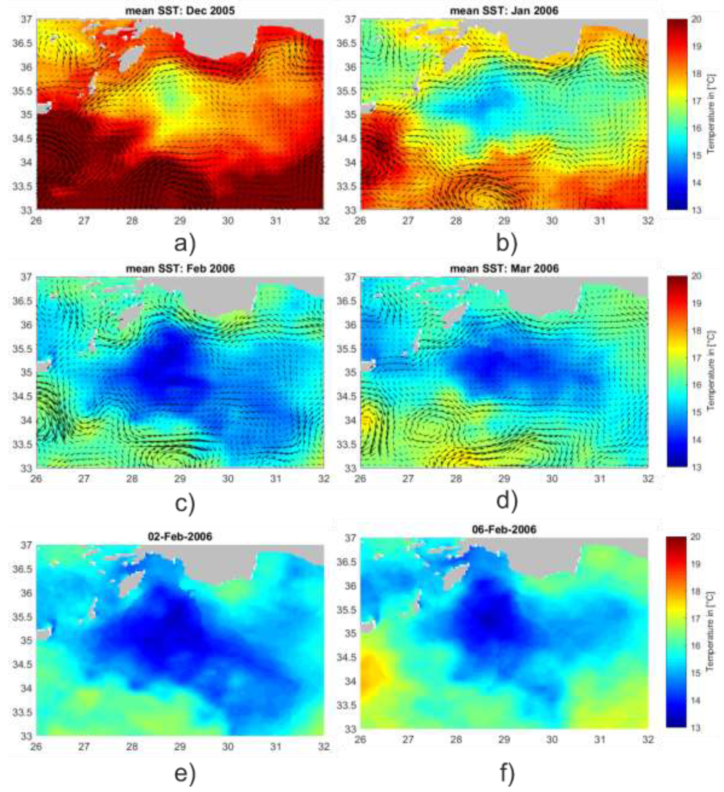
Monthly means of sea surface temperature (SST, °C) and geostrophic currents for (a) December 2005, (b) January, (c) February, and (d) March 2006. Daily SST (°C) of (e) 2 February 2006 and (f) 6 February 2006. Dense water formation and the deep convection event occurred by the end of January until mid-February when SST was lowest.
Figure 10.
Monthly means of sea surface temperature (SST, °C) and geostrophic currents for (a) December 2005, (b) January, (c) February, and (d) March 2006. Daily SST (°C) of (e) 2 February 2006 and (f) 6 February 2006. Dense water formation and the deep convection event occurred by the end of January until mid-February when SST was lowest.

Figure 11.
(a) The temperature and salinity (T/S) plot for float WMO 6900098 from 20 January to 20 February 2006 indicates LDW formation. The additional density line with a potential density value of 29.17 kgm−3 shows the upper deep-water boundary density which corresponds to approximately 1000 m depth for the NWLS [23]. (b) T/S plot for float WMO 6900098 for March 2006 indicates a mixture of LDW and ‘lower range’ LIW formation. Green dots represent depths from 100 to 500 m while blue dots represent depths from 500 to 600 m.

Figure 12.
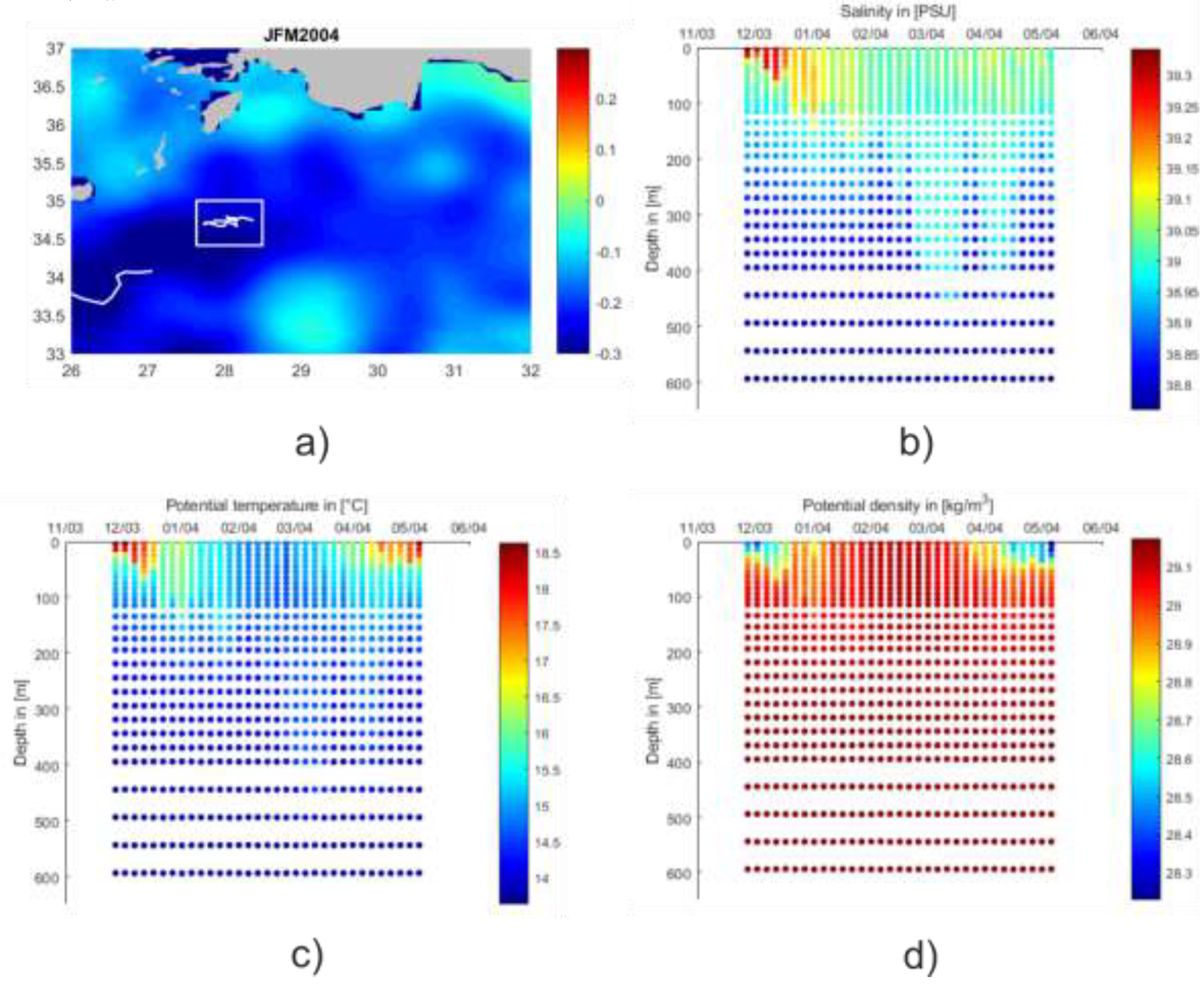
(a) Mean SSH (m) of the Northwestern Levantine Sea and float trajectory of float WMO 6900098 for JFM 2004. (b) Salinity (PSU), (c) potential temperature (°C), and (d) potential density (kgm−3) from December 2003 to April 2004.
Figure 12.
(a) Mean SSH (m) of the Northwestern Levantine Sea and float trajectory of float WMO 6900098 for JFM 2004. (b) Salinity (PSU), (c) potential temperature (°C), and (d) potential density (kgm−3) from December 2003 to April 2004.

Figure 13.
The Turner angle (°) of float WMO 6900098 shows the contribution of salinity and temperature gradients to the density gradient.
Figure 13.
The Turner angle (°) of float WMO 6900098 shows the contribution of salinity and temperature gradients to the density gradient.

Figure 14.
The T/S plot for float WMO 6900098 for JFM 2004 shows LDW and ‘lower range’ LIW formation. Green dots represent depths from 100 to 500 m while blue dots represent depths from 500 to 600 m.
Figure 14.
The T/S plot for float WMO 6900098 for JFM 2004 shows LDW and ‘lower range’ LIW formation. Green dots represent depths from 100 to 500 m while blue dots represent depths from 500 to 600 m.

Figure 15.
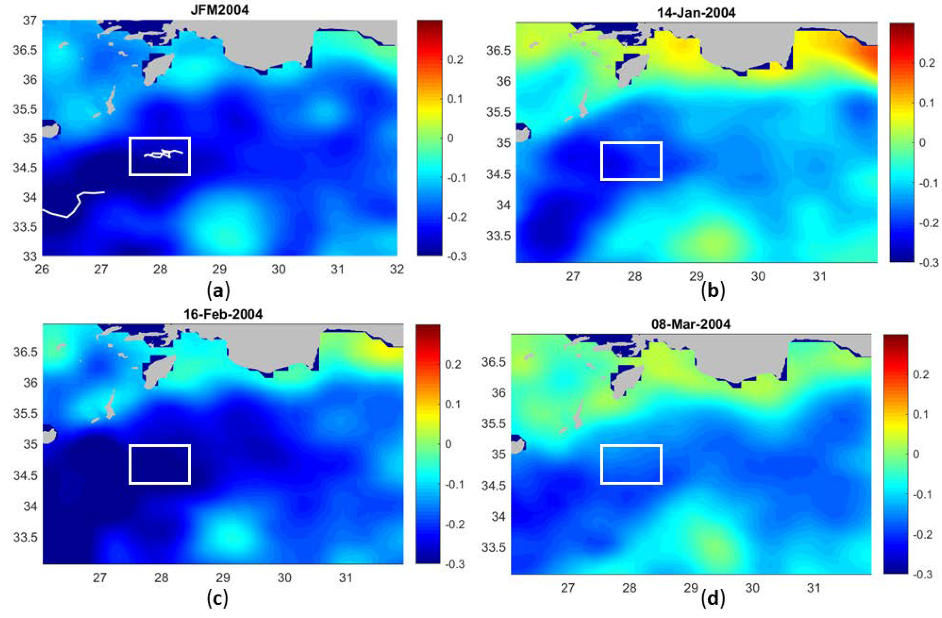
(a) mean SSH (m) for JFM 2004 and float trajectory of float WMO 6900098 (white rectangle). (b) SSH (m) for the 14 January 2004; float profiles show ‘regular’ winter MLDs around 150 m. (c) SSH (m) for the 16 February 2004; float profiles reveal dense water formation to about 350 m; (d) SSH (m) for 8 March 2004; recapping with a newly formed MLD of about 80 m occurred, while the dense water formation event down to 450 m is still captured by the float profile.
Figure 15.
(a) mean SSH (m) for JFM 2004 and float trajectory of float WMO 6900098 (white rectangle). (b) SSH (m) for the 14 January 2004; float profiles show ‘regular’ winter MLDs around 150 m. (c) SSH (m) for the 16 February 2004; float profiles reveal dense water formation to about 350 m; (d) SSH (m) for 8 March 2004; recapping with a newly formed MLD of about 80 m occurred, while the dense water formation event down to 450 m is still captured by the float profile.

Figure 16.
Monthly means of the satellite SST (°C) and absolute geostrophic currents from December 2003 to March 2004. The deep convection event occurred by the end of February and beginning of March 2004 when SST was lowest. The white rectangle shows the position of float WMO 6900098 during JFM 2004.

Figure 17.
(a) Bathymetry of the Northwestern Levantine Sea (m) and float trajectory for float WMO 6900096 during JFM 2007. The red circle indicates the position of the float during March when the deep convection event occurred. Hoevmueller plots of (b) salinity (PSU), (c) potential temperature (°C), and (d) potential density (kgm−3).

Figure 18.
The Turner angle (°) of float WMO 6900098 shows the contribution of salinity and temperature to density change.
Figure 18.
The Turner angle (°) of float WMO 6900098 shows the contribution of salinity and temperature to density change.

Figure 19.
(a–d) Monthly mean of satellite SST (°C) from December 2006 to March 2007. (e) SSH (m) and (f) SST (°C) on 30 March 2007, exhibiting strongest depression of SSH and lowest SST within this area during the whole winter period, coinciding with the deep dense water formation event. The white circle indicates the float position during March 2007.

Figure 20.
T/S plot for float WMO 6900098 for March 2007. Green points indicate depths from 100 to 500 m while blue points indicate depths from 500 to 600 m. The additional density line with a potential density value of 29.17 kgm−3 shows the upper deep-water boundary density while the potential density lines of 29–29.06 × kgm−3 represent the potential density range of typical LIW [6].

Figure 21.
Climatology of the winter (JFM) mean MLD from 2000 to 2018 for the Levantine Sea.

Figure 22.
(a) The white rectangle confines the area of study, the NWLS. Typical LIW formation was found along the Northern coastline (red arrow), while ‘lower range’ LIW and LDW formation was found within submesoscale eddies within the center of RG (black ellipse). (b) This figure, adapted from [15], summarizes the obtained results for winter seasons in the NWLS (yellow rectangle): Dense water formation along the Northern coastline reached intermediate (200–500 m; red line) and deeper layers (500–600 m; dashed red line), while LDW formation within the center of RG reached intermediate and deep layers (at least 1000 m; orange lines).


Table 1.
Pronounced (mixed layer depth (MLD) >250 m) dense water formation events within the center of RG and along the Northern coastline: Area of formation, float WMO, time period, watermass characteristics, and maximum depth during the dense water formation events.
Table 1.
Pronounced (mixed layer depth (MLD) >250 m) dense water formation events within the center of RG and along the Northern coastline: Area of formation, float WMO, time period, watermass characteristics, and maximum depth during the dense water formation events.
| Area of Formation | Float WMO | Time Period | Water Mass Characteristics | Maximum Depth |
|---|---|---|---|---|
| RG | 6900098 | FM 2004 | LDW | At least 600 m, probably 1000 m 1 |
| RG | 6900098 | FM 2005 | LDW | At least 600 m, probably 1000 m 1 |
| RG | 6900098 | JF 2006 | LDW | At least 600 m, probably 1000 m 1 |
| RG | 6900098 | FM 2008 | LDW | At least 600 m, probably 1000 m 1 |
| COAST | 6900098 | M 2007 | LIW | About 550 m |
| COAST | 6900843 | FM 2012 | LIW | About 350 m |
| COAST | 6901824 | FM 2015 | LIW | About 350 m |
| COAST | 6901868 | FM 2016 | LIW | About 300 m |
1 T/S plots show the formation of dense water with a potential density that corresponds to the density of the upper deep boundary layer which is found at approximately 1000 m depth [23].
Table 2.
Argo floats capturing pronounced (MLD >250 m) dense water formation events.
| Float Number | Float Description |
|---|---|
| WMO 6900098 | Apex Profiling Float, Naval Oceanographic Office (NAVO) Alive from 20.07.2003 to 19.04.2009, lifetime approximately 5 years Parking depth (PD)=1000 m; 5 day cycle; |
| WMO 6900843 | Apex Profiling Float, Argomed, Euro-Argo Alive from 03.10.2011 to 31.5.2014, PD=350 m; 5 day cycle; |
| WMO 6901824 | Arvor Profiling Float, Argo Italy, Argomed, Euro-Argo Alive from 04.11.2013 to 03.02.2018, PD=350 m; 5 day cycle; |
| WMO 6901868 | Apex Profiling Float, Argo Italy, Euro-Argo Alive from 01.12.2014 to 29.07.2017. PD=350 m; 5 day cycle; |
© 2019 by the authors. Licensee MDPI, Basel, Switzerland. This article is an open access article distributed under the terms and conditions of the Creative Commons Attribution (CC BY) license (http://creativecommons.org/licenses/by/4.0/).
Share and Cite
MDPI and ACS Style
Kubin, E.; Poulain, P.-M.; Mauri, E.; Menna, M.; Notarstefano, G. Levantine Intermediate and Levantine Deep Water Formation: An Argo Float Study from 2001 to 2017. Water 2019, 11, 1781. https://doi.org/10.3390/w11091781
AMA Style
Kubin E, Poulain P-M, Mauri E, Menna M, Notarstefano G. Levantine Intermediate and Levantine Deep Water Formation: An Argo Float Study from 2001 to 2017. Water. 2019; 11(9):1781. https://doi.org/10.3390/w11091781
Chicago/Turabian StyleKubin, Elisabeth, Pierre-Marie Poulain, Elena Mauri, Milena Menna, and Giulio Notarstefano. 2019. "Levantine Intermediate and Levantine Deep Water Formation: An Argo Float Study from 2001 to 2017" Water 11, no. 9: 1781. https://doi.org/10.3390/w11091781
Note that from the first issue of 2016, this journal uses article numbers instead of page numbers. See further details here.