Estimating the Isotopic Altitude Gradient for Hydrogeological Studies in Mountainous Areas: Are the Low-Yield Springs Suitable? Insights from the Northern Apennines of Italy

 ,
,  , ,
, ,
Abstract
:1. Introduction
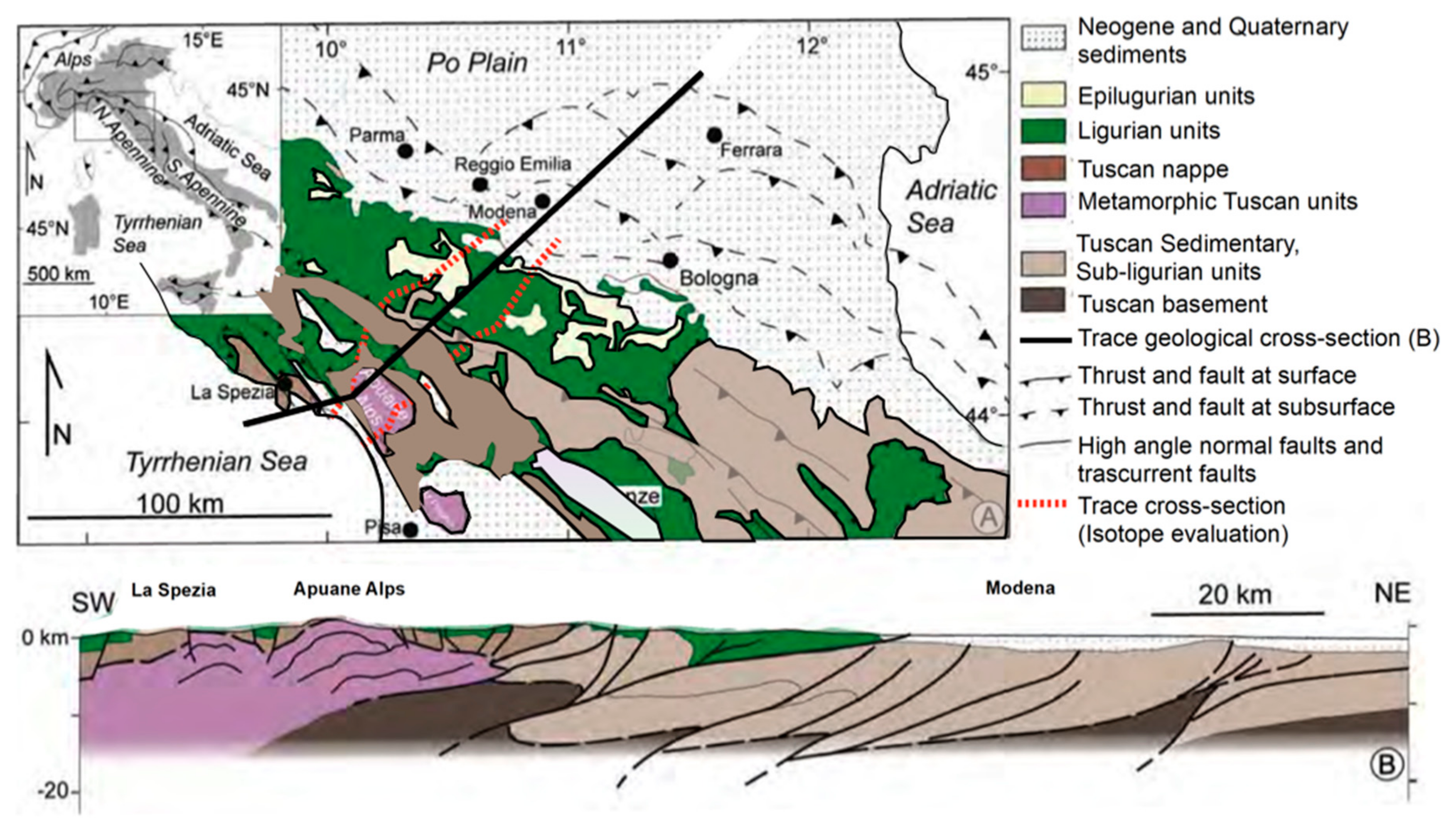
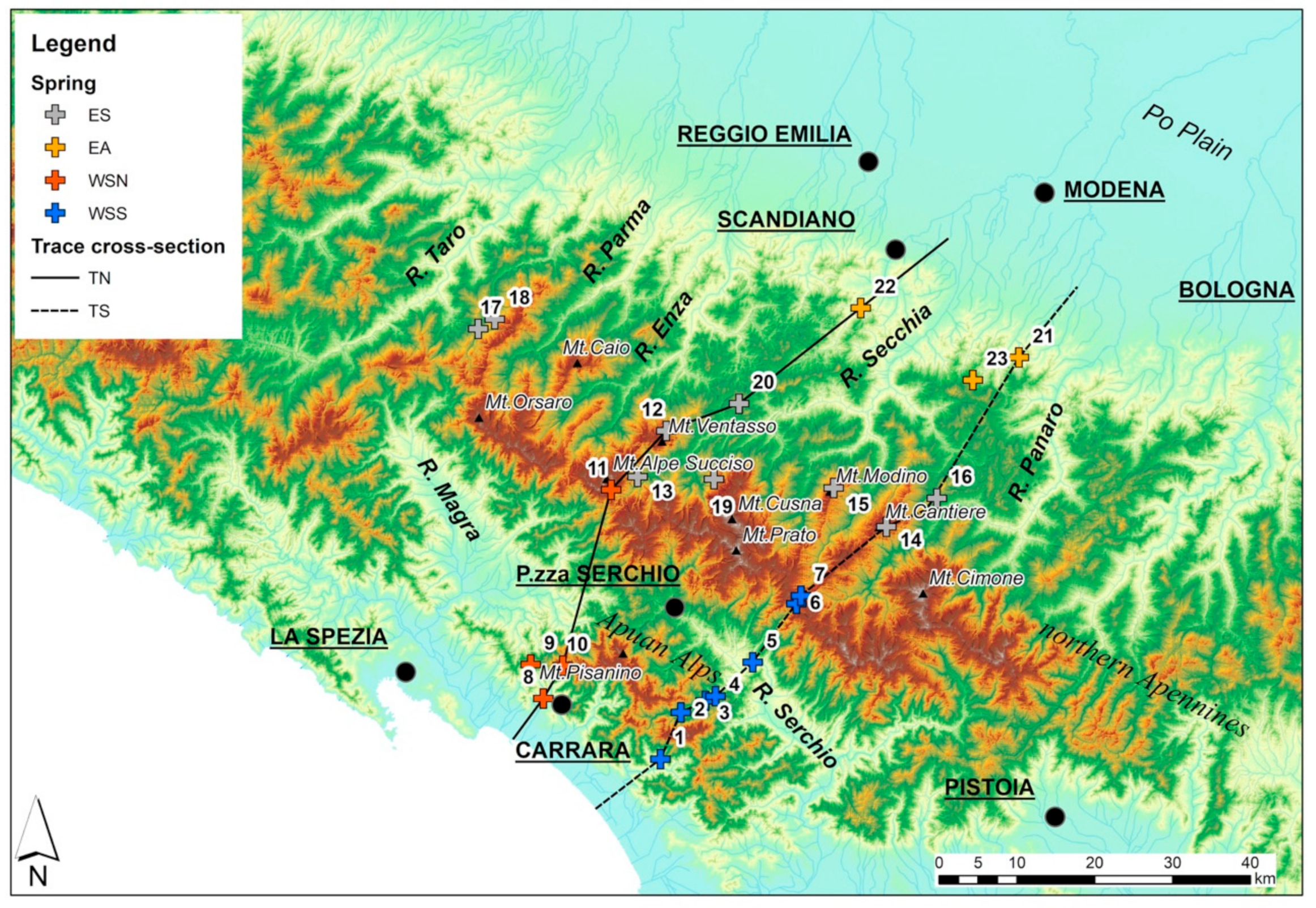
2. Climatic, Geological and Hydrogeological Setting of the Study Area
3. Methods
4. Results
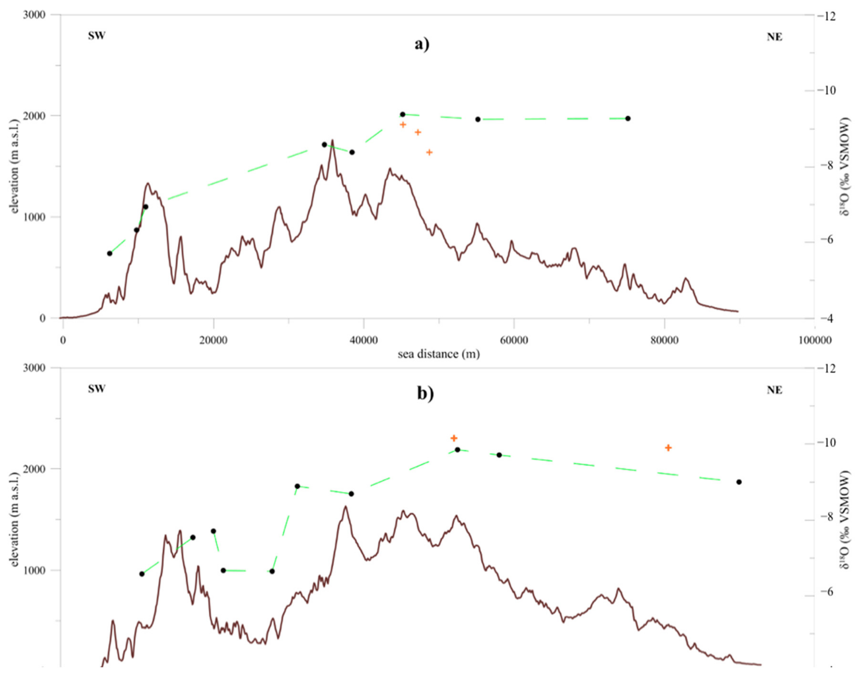
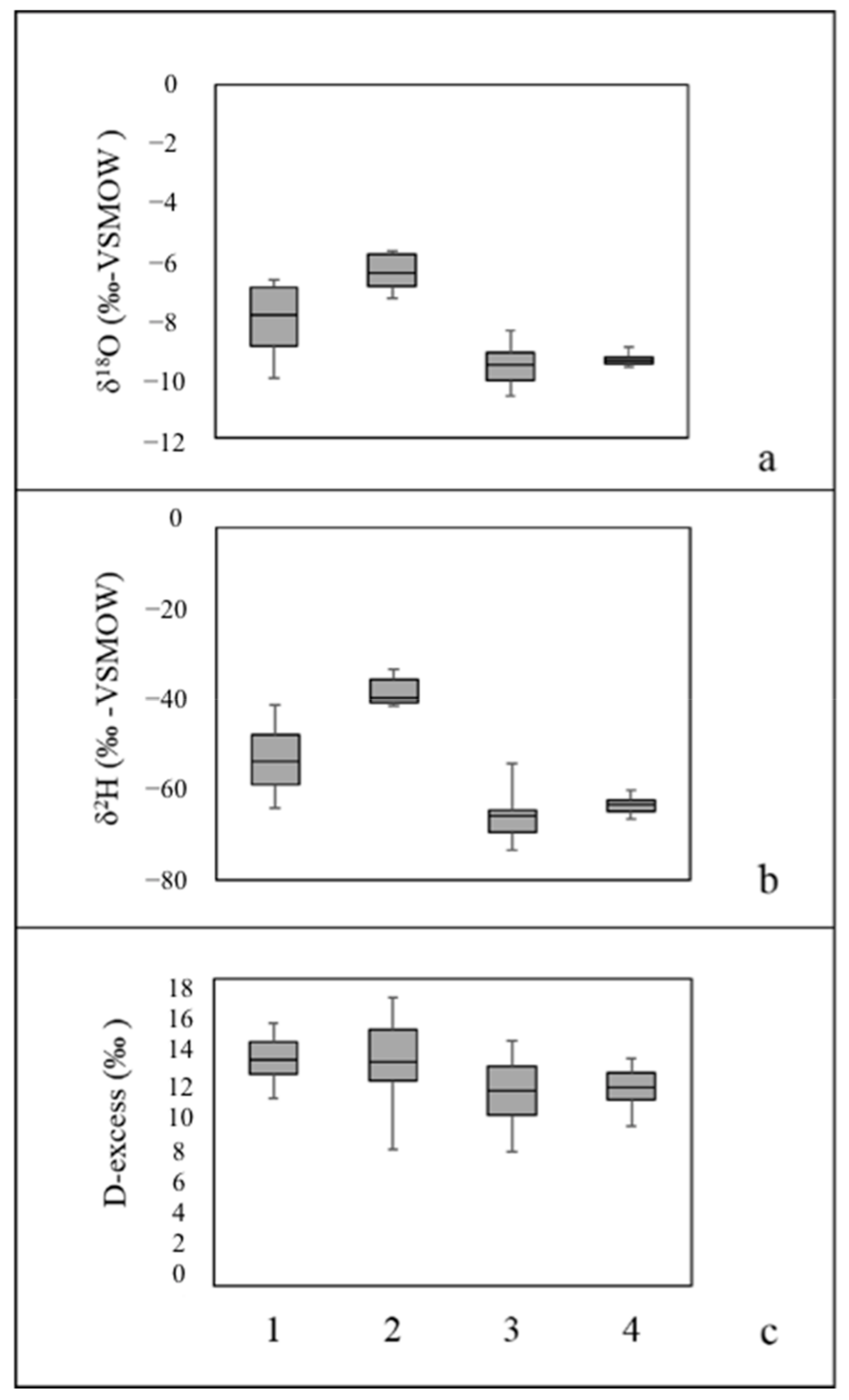
5. Discussion
6. Conclusions
Supplementary Materials
Author Contributions
Funding
Acknowledgments
Conflicts of Interest
References
- Rozanski, K.; Sonntag, C. Vertical distribution of deuterium in atmospheric water vapour. Tellus 1982, 34, 135–141. [Google Scholar] [CrossRef] [Green Version]
- Nanni, T.; Tazioli, A.; Vivalda, P. Problems in the application of environmental isotopes to the hydrogeology of high mountain aquifers. Aqua Mundi 2013, 4, 55–66. [Google Scholar]
- Schemmel, F.; Mikes, T.; Rojay, B.; Mulch, A. The impact of topography on isotopes in precipitation across the Central Anatolian Plateau (Turkey). Am. J. Sci. 2013, 313, 61–80. [Google Scholar] [CrossRef]
- Giustini, F.; Brilli, M.; Patera, A. Mapping oxygen stable isotopes of precipitation in Italy. J. Hydrol. Reg. Stud. 2016, 8, 162–181. [Google Scholar] [CrossRef] [Green Version]
- Le Duy, N.; Heidbüchel, I.; Meyer, H.; Merz, B.; Apel, H. What controls the stable isotope composition of precipitation in the Mekong Delta? A model-based statistical approach. Hydrol. Earth Syst. Sci. 2018, 22, 1239–1262. [Google Scholar] [CrossRef] [Green Version]
- Clark, I.D.; Fritz, P. Environmental Isotopes in Hydrogeology; CRC Press: Boca Raton, FL, USA, 2013; ISBN 978-1-4822-4291-1. [Google Scholar]
- Gat, J.R.; Carmi, I. Evolution of the isotopic composition of atmospheric waters in the Mediterranean Sea area. J. Geophys. Res. 1970, 75, 3039–3048. [Google Scholar] [CrossRef]
- Gonfiantini, R. Chapter 3—Environmental isotopes in lake studies. In The Terrestrial Environment, B; Handbook of Environmental Isotope Geochemistry; Fritz, P., Fontes, J.C., Eds.; Elsevier: Amsterdam, The Netherlands, 1986; pp. 113–168. ISBN 978-0-444-42225-5. [Google Scholar]
- Craig, H. Isotopic Variations in Meteoric Waters. Science 1961, 133, 1702–1703. [Google Scholar] [CrossRef] [PubMed]
- Rozanski, K.; Araguás-Araguá, L.; Gonfiantini, R. Isotopic Patterns in Modern Global Precipitation. In Climate Change in Continental Isotopic Records; Swart, P.K., Lohmann, K.C., McKenzie, J., Savin, S., Eds.; American Geophysical Union (AGU): Washington, DC, USA, 1993; pp. 1–36. ISBN 978-1-118-66402-5. [Google Scholar]
- McGuire, K.; Mcdonnell, J. Stable Isotope Tracers in Watershed Hydrology. In Stable Isotopes in Ecology and Environmental Science, 2nd ed.; Blackwell Publishing: Malden, MA, USA, 2008; pp. 334–374. ISBN 978-0-470-69185-4. [Google Scholar]
- Doveri, M.; Menichini, M.; Cerrina Feroni, A. Gli isotopi stabili dell’acqua come strumento fondamentale nello studio degli acquiferi carsici: Alcuni esempi di applicazione sui complessi carbonatici delle Alpi Apuane (Toscana nw)—Stable water isotope sas fundamental tool in karst aquifer sudies: some results from isotopic applications in the Apuan Alps carbonatic complexes (NW Tuscany, Italy)—IJEGE. Ital. J. Eng. Geol. Environ. 2013, 13, 33–50. [Google Scholar]
- Doveri, M.; Menichini, M.; Scozzari, A. Protection of Groundwater Resources: Worldwide Regulations and Scientific Approaches. In Threats to the Quality of Groundwater Resources: Prevention and Control (The Handbook of Environmental Chemistry); Scozzari, A., Dotsika, E., Eds.; Springer: Berlin/Heidelberg, Germany, 2016; pp. 13–30. ISBN 978-3-662-48596-5. [Google Scholar]
- Montanari, D.; Minissale, A.; Doveri, M.; Gola, G.; Trumpy, E.; Santilano, A.; Manzella, A. Geothermal resources within carbonate reservoirs in western Sicily (Italy): A review. Earth Sci. Rev. 2017, 169, 180–201. [Google Scholar] [CrossRef]
- Tazioli, A. Does the recharge area of a Spring Vary from year to year? Information from the water isotopes. Ital. J. Eng. Geol. Environ. 2017, 2017, 41–56. [Google Scholar]
- Dansgaard, W. Stable isotopes in precipitation. Tellus 1964, 16, 436–468. [Google Scholar] [CrossRef]
- Wassenaar, L.I.; Hendry, M.J.; Chostner, V.L.; Lis, G.P. High Resolution Pore Water δ2H and δ18O Measurements by H2O(liquid)−H2O(vapor) Equilibration Laser Spectroscopy. Environ. Sci. Technol. 2008, 42, 9262–9267. [Google Scholar] [CrossRef] [PubMed]
- Hendry, M.J.; Wassenaar, L.I. Inferring Heterogeneity in Aquitards Using High-Resolution δD and δ18O Profiles. Groundwater 2009, 47, 639–645. [Google Scholar] [CrossRef] [PubMed]
- Stumpp, C.; Hendry, M.J. Spatial and temporal dynamics of water flow and solute transport in a heterogeneous glacial till: The application of high-resolution profiles of δ18O and δ2H in pore waters. J. Hydrol. 2012, 438, 203–214. [Google Scholar] [CrossRef]
- Mussi, M.; Nanni, T.; Tazioli, A.; Vivalda, P.M. The Mt Conero limestone ridge: The contribution of stable isotopes to the identification of the recharge area of aquifers. Ital. J. Geosci. 2017, 136, 186–197. [Google Scholar] [CrossRef]
- Gat, J.R. Oxygen and hydrogen isotopes in the hydrologic cycle. Annu. Rev. Earth Planet. Sci. 1996, 24, 225–262. [Google Scholar] [CrossRef]
- Doveri, M.; Mussi, M. Water Isotopes as Environmental Tracers for Conceptual Understanding of Groundwater Flow: An Application for Fractured Aquifer Systems in the “Scansano-Magliano in Toscana” Area (Southern Tuscany, Italy). Water 2014, 6, 2255–2277. [Google Scholar] [CrossRef]
- Cervi, F.; Corsini, A.; Doveri, M.; Mussi, M.; Ronchetti, F.; Tazioli, A. Characterizing the recharge of fractured aquifers: A case study in a flysch rock mass of the northern apennines (italy). In Engineering Geology for Society and Territory—Volume 3: River Basins, Reservoir Sedimentation and Water Resources; Springer, Cham: Basel, Switzerland, 2015; pp. 563–567. [Google Scholar]
- Vespasiano, G.; Apollaro, C.; De Rosa, R.; Muto, F.; Larosa, S.; Fiebig, J.; Mulch, A.; Marini, L. The Small Spring Method (SSM) for the definition of stable isotope—Elevation relationships in Northern Calabria (Southern Italy). Appl. Geochem. 2015, 63, 333–346. [Google Scholar] [CrossRef]
- Deiana, M.; Cervi, F.; Pennisi, M.; Mussi, M.; Bertrand, C.; Tazioli, A.; Corsini, A.; Ronchetti, F. Chemical and isotopic investigations (δ18O, δ2H, 3H, 87Sr/86Sr) to define groundwater processes occurring in a deep-seated landslide in flysch. Hydrogeol. J. 2018, 26, 2669–2691. [Google Scholar] [CrossRef]
- Longinelli, A.; Selmo, E. Isotopic composition of precipitation in Italy: A first overall map. J. Hydrol. 2003, 270, 75–88. [Google Scholar]
- Zuppi, G.M.; Fontes, J.C.; Letolle, R. Isotopes du milieu et circolations d’eaux sulfureès dans le Latium. In Proceedings of the Isot. Techn. in Groundwater Hydrology; IAEA: Vienna, Austria, 1974; Volume 1, pp. 341–361. [Google Scholar]
- Barbieri, M.; Boschetti, T.; Petitta, M.; Tallini, M. Stable isotope (2H, 18O and 87Sr/86Sr) and hydrochemistry monitoring for groundwater hydrodynamics analysis in a karst aquifer (Gran Sasso, Central Italy). Appl. Geochem. 2005, 20, 2063–2081. [Google Scholar] [CrossRef]
- Conversini, P.; Tazioli, G.S. Indagini idrogeologiche nella media e alta valle del fiume Menotre, Umbria orientale. Atti Tic. Sci. Terra 1993, 36, 153–164. [Google Scholar]
- Tazioli, A.; Mosca, M.; Tazioli, G.S. Location of recharge area of Gorgovivo Spring, Central Italy. A contribution from isotope hydrology. In Proceedings of the International Symposium “Advances in Isotope Hydrology and Its Role in Sustainable Water Resources Management (IHS-2007)”; IAEA: Vienna, Austria, 2007; pp. 27–35. [Google Scholar]
- Tazioli, A.; Conversini, P.; Peccerillo, A. Hydrogeological and geochemical characterisation of the Rock of Orvieto. Environ. Earth Sci. 2012, 66, 55–65. [Google Scholar] [CrossRef]
- Deiana, M.; Mussi, M.; Ronchetti, F. Discharge and environmental isotope behaviours of adjacent fractured and porous aquifers. Environ. Earth Sci. 2017, 76, 595. [Google Scholar] [CrossRef]
- Cervi, F.; Ronchetti, F.; Doveri, M.; Mussi, M.; Marcaccio, M.; Tazioli, A. The use of stable water isotopes from rain gauges network to define the recharge areas of springs: Problems and possible solutions from case studies in the northern Apennines. Geoing. Ambient. Min. 2016, 149, 19–26. [Google Scholar]
- Molli, G. Northern Apennine—Corsica orogenic system: An updated overview. Geol. Soc. Lond. Spec. Publ. 2008, 298, 413–442. [Google Scholar] [CrossRef]
- Civita, M.; Forti, P.; Marini, P.; Meccheri, M.; Micheli, L.; Piccini, L.; Pranzini, G. Note Illustrative Della Carta Della Vulnerabilità All’inquinamento Degli Acquiferi Delle Alpi Apuane—Pollution Vulnerability Map for the Aquifers of the Apuane Alps a Brief Guide; SELCA: Firenze, Italy, 1991. [Google Scholar]
- Baldacci, F.; Cecchini, S.; Lopane, G.; Raggi, G. Le risorse idriche del bacino del Fiume Serchio ed il loro contributo all’alimentazione dei bacini idrografici adiacenti. Mem. Della Soc. Geol. Ital. 1993, 49, 365–391. [Google Scholar]
- Antolini, G.; Pavan, V.; Tomozeiu, R.; Marletto, V. Atlante climatico dell’Emilia-Romagna. Casma Tipolito srl–Bologna, Italy, 1961–2015. Available online: https://www.arpae.it/cms3/documenti/_cerca_doc/meteo/clima/Atlante_climatico_1961-2015.pdf (accessed on 23 August 2019).
- Longinelli, A.; Anglesio, E.; Flora, O.; Iacumin, P.; Selmo, E. Isotopic composition of precipitation in Northern Italy: Reverse effect of anomalous climatic events. J. Hydrol. 2006, 329, 471–476. [Google Scholar] [CrossRef]
- Zuppi, G.M.; Bortolami, G. Hydrogeology: A privileged field for environmental stable isotopes applications. Some Italian examples. Rend. Della Soc. Ital. Mineral. Petrol. 1983, 38, 1197–1212. [Google Scholar]
- Boccaletti, M.; Elter, P.; Guazzone, G. Polarita strutturali delle Alpi e dell’Appennino settentrionale in rapporto all’inversione di una zona di subduzione nord-tirrenica. Mem. Della Soc. Geol. Ital. 1971, 10, 371–378. [Google Scholar]
- Carmignani, L.; Kligfield, R. Crustal extension in the Northern Apennines: The transition from compression to extension in the Alpi Apuane Core Complex. Tectonics 1990, 9, 1275–1303. [Google Scholar] [CrossRef]
- Molli, G.; Cortecci, G.; Vaselli, L.; Ottria, G.; Cortopassi, A.; Dinelli, E.; Mussi, M.; Barbieri, M. Fault zone structure and fluid—Rock interaction of a high angle normal fault in Carrara marble (NW Tuscany, Italy). J. Struct. Geol. 2010, 32, 1334–1348. [Google Scholar] [CrossRef]
- Corsini, A.; Cervi, F.; Ronchetti, F. Weight of evidence and artificial neural networks for potential groundwater spring mapping: An application to the Mt. Modino area (Northern Apennines, Italy). Geomorphology 2009, 111, 79–87. [Google Scholar] [CrossRef]
- Gargini, A.; De Nardo, M.T.; Piccinini, L.; Segadelli, S.; Vincenzi, V. Spring discharge and groundwater flow systems in sedimentary and ophiolitic hard rock aquifers: Experiences from Northern Apennines (Italy). In Fractured Rock Hydrogeology; IAH—Selected Papers on Hydrogeology; Sharp, J.M., Ed.; CRC Press: Boca Raton, FL, USA, 2014; pp. 129–145. ISBN 978-1-138-00159-6. [Google Scholar]
- Molli, G.; Doveri, M.; Manzella, A.; Bonini, L.; Botti, F.; Menichini, M.; Montanari, D.; Trumpy, E.; Ungari, A.; Vaselli, L. Surface-subsurface structural architecture and groundwater flow of the Equi Terme hydrothermal area, northern Tuscany Italy. Ital. J. Geosci. 2015, 134, 442–457. [Google Scholar] [CrossRef]
- Doveri, M.; Piccini, L.; Menichini, M. Hydrodynamic and Geochemical Features of Metamorphic Carbonate Aquifers and Implications for Water Management: The Apuan Alps (NW Tuscany, Italy) Case Study. In Karst Water Environment; The handbook of environmental chemistry; Younos, T., Schreiber, M., Kosič Ficco, C., Eds.; Springer, Cham: Basel, Switzerland, 2019; ISBN 978-3-319-77368-1. [Google Scholar]
- Chiesi, M.; De Waele, J.; Forti, P. Origin and evolution of a salty gypsum/anhydrite karst spring: The case of Poiano (Northern Apennines, Italy). Hydrogeol. J. 2010, 18, 1111–1124. [Google Scholar] [CrossRef]
- Gargini, A.; Vincenzi, V.; Piccinini, L.; Zuppi, G.M.; Canuti, P. Groundwater flow systems in turbidites of the Northern Apennines (Italy): Natural discharge and high speed railway tunnel drainage. Hydrogeol. J. 2008, 16, 1577–1599. [Google Scholar] [CrossRef]
- Cervi, F.; Borgatti, L.; Dreossi, G.; Marcato, G.; Michelini, M.; Stenni, B. Isotopic features of precipitation and groundwater from the Eastern Alps of Italy: Results from the Mt. Tinisa hydrogeological system. Environ. Earth Sci. 2017, 76, 410. [Google Scholar] [CrossRef]
- Ronchetti, F.; Borgatti, L.; Cervi, F.; Gorgoni, C.; Piccinini, L.; Vincenzi, V.; Corsini, A. Groundwater processes in a complex landslide, northern Apennines, Italy. Nat. Hazards Earth Syst. Sci. 2009, 9, 895–904. [Google Scholar] [CrossRef] [Green Version]
- Freeze, R.A.; Cherry, J.A. Groundwater; Prentice-Hall: Englewood cliffs, NJ, USA, 1979; ISBN 978-0-13-365312-0. [Google Scholar]
- Cervi, F.; Borgatti, L.; Martinelli, G.; Ronchetti, F. Evidence of deep-water inflow in a tectonic window of the northern Apennines (Italy). Environ. Earth Sci. 2014, 72, 2389–2409. [Google Scholar] [CrossRef]
- Epstein, S.; Mayeda, T. Variation of O18 content of waters from natural sources. Geochim. Cosmochim. Acta 1953, 4, 213–224. [Google Scholar] [CrossRef]
- Coleman, M.L.; Shepherd, T.; Durham, J.J.; Rouse, J.E.; Moore, G.R. Reduction of water with zinc for hydrogen isotope analysis. Anal. Chem. 1982, 54, 993–995. [Google Scholar] [CrossRef]
- Mussi, M.; Leone, G.; Nardi, I. Isotopic geochemistry of natural waters from the Alpi Apuane—Garfagnana area, Northern Tuscany, Italy. Mineral. Petrogr. Acta 1998, 41, 163–178. [Google Scholar]
- Guan, H.; Simmons, C.T.; Love, A.J. Orographic controls on rain water isotope distribution in the Mount Lofty Ranges of South Australia. J. Hydrol. 2009, 374, 255–264. [Google Scholar] [CrossRef]
- Doveri, M.; Stenni, B.; Petrini, R.; Giannecchini, R.; Dreossi, G.; Menichini, M.; Ghezzi, L. Oxygen and hydrogen isotopic composition of waters in a past-mining area of southern Apuan Alps (Italy): Hydrogeological characterization and implications on the fate of potentially toxic elements. J. Geochem. Explor. 2019, 205, 106338. [Google Scholar] [CrossRef]


| No. on Map | Name of the Spring | Number of Values | Emerging Altitude | Mean Altitude of the Watershed | Oxygen-18 (Low Flow Value) | +/− | Deuterium (Low Flow Value) | +/− | d-excess |
|---|---|---|---|---|---|---|---|---|---|
| 1 | km 14.6 | 8 | 475 | 700 | −6.58 | 0.16 | −40.6 | 12.04 | |
| 2 | km 29.2 | 7 | 600 | 800 | −7.54 | 0.05 | −47.4 | 0.23 | 12.92 |
| 3 | km 32.6 | 6 | 425 | 800 | −7.71 | 0.09 | −49.5 | 0.6 | 12.18 |
| 4 | km 35.4 | 8 | 370 | 400 | −6.67 | 0.11 | −44.2 | 0.5 | 9.16 |
| 5 | S. francesco | 9 | 490 | 510 | −6.65 | 0.05 | −41.4 | 0.3 | 11.8 |
| 6 | La fredda | 9 | 1540 | 1650 | −8.89 | 0.13 | −56.2 | 0.3 | 14.92 |
| 7 | Imbrancamento | 14 | 1350 | 1480 | −8.69 | 0.26 | −55.3 | 0.7 | 14.22 |
| 8 | Fontana fredda | 17 | 150 | 300 | −5.7 | 0.06 | −36.2 | 0.7 | 9.4 |
| 9 | Maestà | 10 | 800 | 810 | −6.32 | 0.29 | −35.6 | 0.5 | 14.96 |
| 10 | Acqua sparta | 10 | 1275 | 1350 | −6.93 | 0.23 | −43.3 | 0.4 | 12.14 |
| 11 | Secchia springs | 2 | 1500 | 1700 | −8.57 | 0.11 | −56.4 | 0.2 | 12.16 |
| 12 | Cadoniche | 1 | 1325 | 1350 | −9.37 | ||||
| 13 | Collagna | 7 | 850 | 960 | −8.37 | 0.13 | −53.7 | 1.6 | 13.26 |
| 14 | Mt Cantiere | 8 | 1170 | 1450 | −9.85 | 0.08 | −65.6 | 0.8 | 13.2 |
| 15 | Venano | 7 | 1180 | 1280 | −10.15 | 0.1 | −67.07 | 1.5 | 14.13 |
| 16 | Borra | 1 | 900 | 1100 | −9.71 | ||||
| 17 | Fugazzolo | 1 | 1017 | 1000 | −8.9 | ||||
| 18 | Berceto | 13 | 825 | 880 | −8.37 | 0.21 | −53.3 | 0.3 | 13.66 |
| 19 | Montecagno | 22 | 1050 | 1100 | −9.10 | 0.05 | −62.96 | 0.3 | 9.84 |
| 20 | Bismantova | 14 | 800 | 920 | −9.24 | 0.38 | −61.9 | 0.6 | 12.02 |
| 21 | M. di Puianello | 2 | 350 | 375 | −9.00 | 0.18 | −60.2 | 0.4 | 11.8 |
| 22 | Lusino | 7 | 325 | 440 | −9.26 | 0.11 | −64.7 | 0.5 | 9.38 |
| 23 | La fontanina | 1 | 650 | 725 | −9.9 | 0.12 |
© 2019 by the authors. Licensee MDPI, Basel, Switzerland. This article is an open access article distributed under the terms and conditions of the Creative Commons Attribution (CC BY) license (http://creativecommons.org/licenses/by/4.0/).
Share and Cite
Tazioli, A.; Cervi, F.; Doveri, M.; Mussi, M.; Deiana, M.; Ronchetti, F. Estimating the Isotopic Altitude Gradient for Hydrogeological Studies in Mountainous Areas: Are the Low-Yield Springs Suitable? Insights from the Northern Apennines of Italy. Water 2019, 11, 1764. https://doi.org/10.3390/w11091764
Tazioli A, Cervi F, Doveri M, Mussi M, Deiana M, Ronchetti F. Estimating the Isotopic Altitude Gradient for Hydrogeological Studies in Mountainous Areas: Are the Low-Yield Springs Suitable? Insights from the Northern Apennines of Italy. Water. 2019; 11(9):1764. https://doi.org/10.3390/w11091764
Chicago/Turabian StyleTazioli, Alberto, Federico Cervi, Marco Doveri, Mario Mussi, Manuela Deiana, and Francesco Ronchetti. 2019. "Estimating the Isotopic Altitude Gradient for Hydrogeological Studies in Mountainous Areas: Are the Low-Yield Springs Suitable? Insights from the Northern Apennines of Italy" Water 11, no. 9: 1764. https://doi.org/10.3390/w11091764