Using Soil, Plant, Topographic and Remotely Sensed Data to Determine the Best Method for Defining Aflatoxin Contamination Risk Zones within Fields for Precision Management

Abstract

Contamination of crops by aflatoxins (AFs) is a real risk in the South-Eastern USA. Contamination risk at the county level based on soil type and weather in different years has been investigated. However, defining AFs contamination risk zones within fields has not yet been attempted. Drought conditions, particularly within the month of June have been linked to high levels of AFs contamination at the county level. Soil characteristics and topography are the factors influencing drought status that vary most within fields. Here, soil, plant, topography and remotely sensed information are used to define AFs contamination risk zones within two fields using different approaches. Normalized difference vegetation index (NDVI) data were used to indicate potential droughty areas and thermal IR data from LandSat imagery were used to identify hot areas. Topographic variables were also computed. Comparison tests showed that a combination of regression analysis of soil, plant and imagery data and bi-variate local Moran’s I analysis of NDVI and Thermal IR data from several years was the best way to define zones for mean and maximum AFs levels. An approach based on principal components analysis of soil, plant and imagery data from 2010, a high-risk year, was best for defining zones for minimum AFs levels. Analysis of imagery from several years suggested that the zones are likely to be relatively stable in time and could be defined using only freely available sensor, topographic and soil series data. Once defined, such zones can be managed to increase profitability and reduce waste.

1. Introduction

Aflatoxins (AFs) are mycotoxins produced by Aspergillus flavus and Aspergillus parasiticus fungi [1] which can contaminate corn [2] and other staple crops like millet, rice, sorghum and wheat [1,3,4,5]. They can cause liver cancer in humans and animals [6,7] so strict legislative limits on the levels allowed in grain exist [8,9]. Globally, Liu and Wu [10] estimated that there are 16–31 times higher liver cancer mortality rates in less-developed countries that can be attributed, at least in part to AFs contamination of food. In the USA, the United States Federal Food and Drug Administration (FDA) has two general limits of 20 ppb and 100 ppb for total AFs in animal feed and 200 ppb and 300 ppb limits for animals of particular species, age and use [11]. The 20 ppb limit restricts the use of corn, peanut products and cottonseed meal to feeds for dairy or immature animals [11]. The 100 ppb limit restricts the use of corn and peanut products for breeding beef cattle, swine, or mature poultry [11]. The 200 ppb limit restricts the use of corn and peanut products to finishing swine of 100 lbs or more [11] and the 300 ppb limit restricts the use of these products to finishing beef cattle [11]. While the safety of food products is dictated by such thresholds, AFs are expensive to measure [12] so levels are usually measured at harvest and the whole crop is accepted or rejected based on the average concentration of a bulked sample [13,14] leading to large quantities of wasted grain and decreased profits for farmers.

Contamination by AFs of crops in the field has been shown to be driven by high temperatures and drought conditions [15]. Summer corn crops in the southern states of the USA can be particularly susceptible to AFs contamination due to rainfall variability, light-textured soils and lack of irrigation infrastructure [16]. Salvacion et al. [17] showed that in southern Georgia (GA), USA, the rainfall (RF) and maximum temperatures (TMax) in June, the key mid-silk growth period in corn, were particularly important to contamination risk. The work of Kerry et al. [18] and Yoo et al. [19] also suggested that June RF, June TMax and soil drainage characteristics are key to contamination levels in southern GA. The increased AFs contamination risk under hot, dry conditions suggests that high risk areas are likely to expand under future climate change scenarios. Indeed, this has been shown for Europe [20] and the State of GA, USA [21]. Rising temperatures are also important to AFs contamination risk in stored grain with increased insect infestations likely as temperatures rise [22]. There is a need for improved forecasting of AFs contamination to improve management strategies of crops within seasons [23].

Using a 30-year survey of corn AFs levels for southern GA, Kerry et al. [18] investigated the total level of contamination risk at the county scale looking at the following risk factors: June TMax [17], June RF [17], percentage of well- and excessively-drained soils [24,25] and the percentage of county area in corn production. Yoo et al. [19] used profile regression to determine the relative importance of each risk factor and to determine if satellite imagery data were likely to be useful for determining risk. Normalized difference vegetation index (NDVI) data from aerial imagery and satellites have been used to indicate yield and plant health response to drought conditions [26,27] and thermal infrared (IR) data have also been used to indicate locations with drought stress [28,29]. Low NDVI values indicate low chlorophyll levels which can indicate drought or nitrogen deficiency. Yoo et al. [19] found that at the county level, NDVI and Thermal IR data behaved as expected with low NDVI levels corresponding to areas with low June RF and high thermal IR values corresponding to areas with high temperatures. Kerry et al. [30] used weather data with NDVI and thermal IR data from satellite imagery for corn growing pixels to identify the highest risk areas within counties of southern Georgia over several of years. Pixels with low NDVI (low June RF) and high thermal IR (high June TMax) values were shown to be at greater risk of AFs contamination and areas that exceeded the 20 ppb and 100 ppb thresholds in the most years showed the highest frequency of years with low NDVI and high Thermal IR. Yoo et al. [19] also showed that the risk of breaching the 100 ppb FDA threshold was increased where there were larger percentages of excessively drained soils in hot dry years.

This study aims to build on previous research that has identified key factors that influence AFs contamination and examine how these vary spatially within individual fields in relation to AFs contamination for an individual high-risk year. The aim is to identify drought prone areas that are at risk of AFs contamination using expensive and free or inexpensive data to show that both types of data can identify similar zones. With inexpensive methods for farmers to define zones, they can then reduce waste and increase their profit. Identification of zones with different contamination risk can lead to differential crop management strategies. At planting, lower planting densities could be employed in high-risk zones and varieties more resistant to Aspergillus infection and more drought resistant could be planted [19]. During the season, more irrigation and targeted fungicide application could take place in the higher risk areas and at harvest, grain from different risk zones could be harvested and stored separately as micro batches so that the average concentrations of most micro batches of grain does not exceed legislative limits and therefore the whole crop would not be rejected or have to be diverted to a less lucrative use.

Given the expense of determining the level of AFs in samples [12] and the cost of soil and plant analysis, dense spatial and temporal studies at the field scale are prohibitively expensive for individual farmers. It is necessary to determine if the same factors that determine risk at the county level are relevant at the field scale and if freely available remotely sensed data can be used to identify risk zones. AFs Contamination risk at the field scale has not been investigated previously and much AFs research is lab-based determining the optimal conditions for fungal growth and toxin production.

Weather conditions in terms of June TMax and June RF are relatively constant within farmer’s fields, although there may be differences in maximum temperatures that are associated with topographic attributes such as aspect. There are also differences in soil moisture related to degree or slope, topographic position and soil texture. Greater contamination risk within fields is likely in areas with light-textured soil, shedding topographic positions and aspects with the greatest evapotranspiration potential. These are relatively permanent features of fields thus patterns of AFs contamination risk are likely to be stable in time and consistent with the most drought-prone areas in the field. As soil survey and field observation are expensive, field observations were made in one high-risk season: 2010 and free remotely sensed, DEM and soil survey data were used to determine if the risk zones were likely to be stable in time. This study investigates the spatial variation in the relative risk of AFs contamination within two non-irrigated fields in south-eastern Alabama (AL), USA. The aims of this work are to compare different methods of identifying AFs risk zones based on field and imagery data from 2010, and to determine if those zones are likely to be stable in time based on imagery from 2006 to 2011 and 2019. If AFs contamination risk zones can be successfully defined within fields they have the potential to allow farmers to get a higher price for their crop and result in less wasted grain in areas, like the South-Eastern USA, that are at high risk of AFs contamination in some years.

2. Materials and Methods

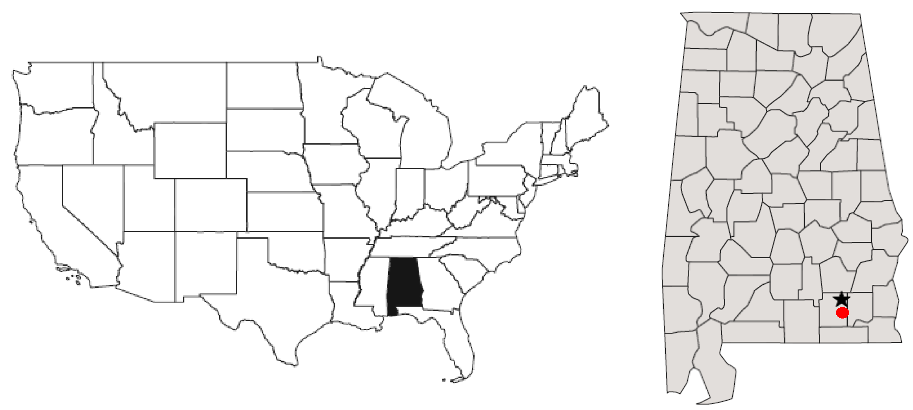
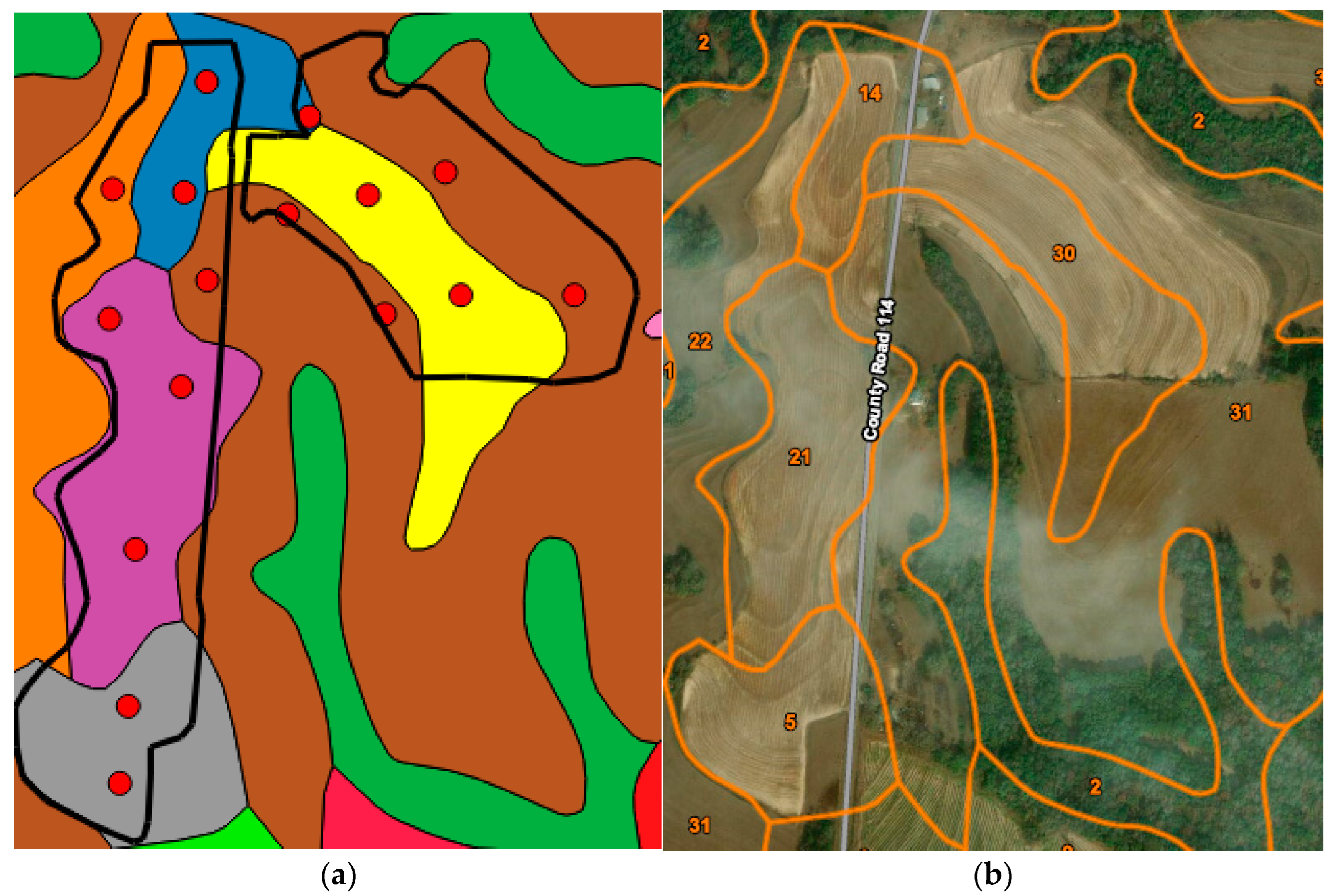
2.1. Field Observations

Total AFs concentrations (ppb) were measured in two non-irrigated corn fields in South-Eastern Alabama (AL), USA (31.530504° N and −85.871256° W) at harvest in the 2010 growing season, a high-risk season for AFs contamination. The fields were located in Coffee County about 23 km north of Enterprise, AL (Figure 1). Each 13-hectare field was divided into zones based on soil type and elevation (Figure 2) and two locations within each zone (a total of 16 locations where samples were taken) were assessed for AFs with three replicates measured at each location. For each location, the ten upper-most corn ears were hand-harvested at maturity from the center rows. Ears were machine shelled. The grain from the 10 ears collected at each location was then manually mixed and a sub-sample (250 g) was obtained for AFs assessment [31,32]. The 250 g sub-sample was ground to <2 mm with a Thomas-Wiley Laboratory Mill, model 4 (Swedesboro, NJ, USA). Total AFs quantitative assessment was done on 10 g of ground corn per treatment using the Veratox test (Neogen Corp., Lansing, MI, USA). The detection limit and quantitation range of the Veratox test is equal to 1.4 and 5 to 50 µg kg⁻¹, respectively. Duplicates were run for approximately 10% of the samples to verify AFs concentration [32].

Figure 2b shows the soil series present in each field and

Table 1. Summary details of soil series at the field site.

Soil Series Number	Name	Slope (%)	Drainage Class	Landform	Profile—Horizon Depths (cm) and USDA Textural Class	Prime Farmland?
5	Bonifay LS	1–5	Well-drained	Ridges	H1—0–115 cm: LS H2—115–180 cm: SCL	No
14	Fuquay LS	0–5	Well-drained	Interfluves	Ap—0–25 cm: LS E1—25–56 cm: LS E2—56–70 cm: LS Bt1—70–90 cm: SCL Bt2—90–110 cm: SCL Btv—110–165 cm: SCL	No
21	Orangeburg SL	2–5	Well-drained	Ridges	A—0–20 cm: SL Bt1—20–150 cm: SCL Bt2—150–200 cm: SCL	Yes
22	Orangeburg SL	5–8	Well-drained	Ridges	A—0–20 cm: SL Bt1—20–150 cm: SCL Bt2—150–200 cm: SCL	Yes
30	Troup LS	1–5	Somewhat excessively drained	Ridges	H1—0–145 cm: LS H2—145–215 cm: SL	No
31	Troup LS	5–8	Somewhat excessively drained	Hillslopes, Ridges	Ap—0–8 cm: LS E—8–130 cm: LS Bt—130–200 cm: SCL	No

SCL—Sandy Clay Loam, SC—Sandy Clay, LS—Loamy Sand.

gives the details of the soil series by corresponding number.

On 21 July 2010, soil samples were collected at 10, 20, 30, 40, 60 and 100 cm depth at each sample location. Gravimetric water content of the soil was determined by drying at 105 °C until consistent weights were reached. Gravimetric water contents were converted to volumetric water content (VWC) using soil bulk density values and then the VWC values for the top three depths were averaged to give Top-soil VWC (0–30 cm) and the three deeper depths were averaged to produce sub-soil VWC (40–100 cm). Soil type was extracted from a soil survey map (https://websoilsurvey.nrcs.usda.gov/app/WebSoilSurvey.aspx accessed on 14 August 2022).

The soil plant analysis development (SPAD) chlorophyll meter is one of the most commonly used diagnostic tools to measure crop greenness on the ground within fields. Leaf chlorophyll has been used to infer moisture status of a plant but, perhaps more commonly, it has been used to indicate leaf nitrogen status [33]. There is thus, an inability to determine if a plant is less green due to lack of water or lack of nitrogen, but dry conditions can reduce plant nitrogen uptake [34]. Leaf chlorophyll (SPAD) was measured for the leaves of four plants at each sample location on 21 July 2010 and averaged to give an indication of drought status of plants.

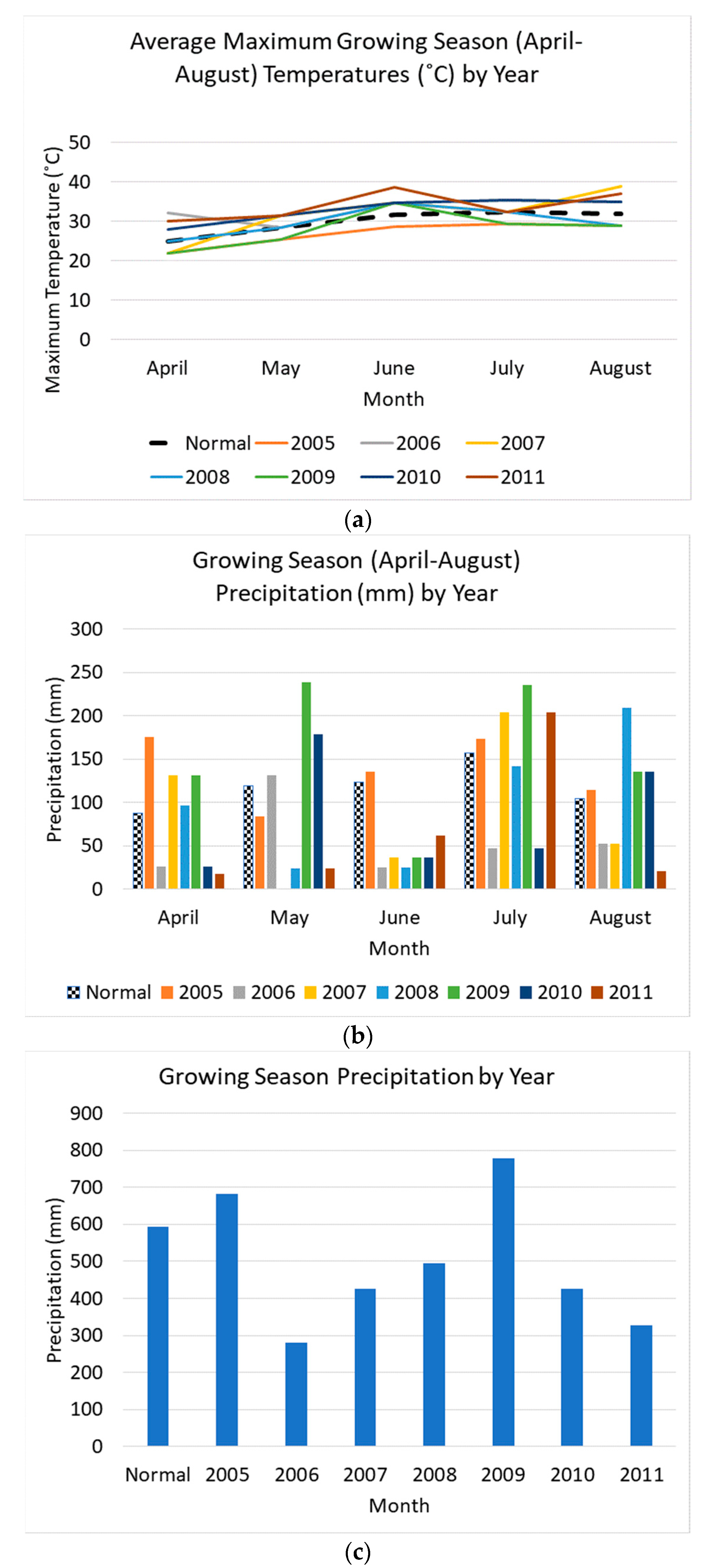
2.2. Weather, Topography and Remotely Sensed Data

The 30-year climate normals of average maximum monthly temperatures and precipitation totals for the nearest weather station with sufficient data, Enterprise, AL (Figure 1) were obtained from http://www.sercc.com/cgi-bin/sercc/cliMAIN.pl?al2675 (accessed on 14 August 2022). There was a lot of missing data for this weather station and nearby stations for the 2005–2012 study period, so monthly values were extracted from gridded data at https://prism.oregonstate.edu/recent/monthly.php (accessed on 14 August 2022). Values were extracted from monthly contour maps of average Tmax and total RF. As the data were extracted from contour maps there is an upper and lower bound to each contour resulting in some uncertainty in the weather data. For monthly Tmax, the uncertainty was a maximum of 2.5 °C and for monthly RF the uncertainty was at a maximum of 50 mm. Figure 3 shows the monthly Tmax and RF values extracted in this way for the 2005–2011 growing seasons (April–August) and the 30 year normal for Enterprise, AL.

A freely available, 30 m digital elevation model (DEM), AW3D30 v3.1 [35] produced by the Japan Aerospace Exploration Agency (JAXA) (https://www.eorc.jaxa.jp/ALOS/en/aw3d30/index.htm accessed on 14 August 2022) was used to calculate the wetness index [36] and a topographic wetness index (TWI) [37]. SAGA GIS software [38] was used for these calculations and included other outputs such as the modified catchment area (MCA).

LandSat 5 (30 m) data for all cloud-free dates in the 2006 to 2011 growing seasons (April-August) for all pixels within the field boundaries were obtained from USGS EarthExplorer (https://earthexplorer.usgs.gov/ accessed on 14 August 2022). The imagery was processed to generate surface reflectances which were then used to calculate NDVI and thermal IR. Sentinel-2 NDVI (10 m) and normalized difference red edge (NDRE) data were also extracted and calculated from an image taken on 14 June 2019 to determine if the increased spatial, and spectral resolution of the Sentinel data could be helpful in identifying within-field drought-prone areas.

2.3. Statistical Analysis

Based on the three replicate values at each sample location, minimum (MIN), maximum (MAX) and mean (MEAN) AFs values were determined for each sampling point and were kriged to a 30 m grid (Figure 4a–c). Kriging is usually not possible with so few data points, especially if collected on a grid as the variograms can be a pure nugget or very erratic [39] (Figure 5). Kerry and Oliver [40] however, showed how sparse, spatially structured data could be kriged with variograms from more densely sampled, related data. Kerry and Oliver [40] used standardized variograms to krige such data. However, the variance of a data set can be used to determine the variogram sill and thus the data can be kriged with a model and proportion of nugget variance derived from dense data without standardization of the data. Soil VWC and SPAD measurements were also kriged from the sample locations to a 30 m grid.

Pearson correlations between kriged field data and remotely sensed data were examined. Three best subset regressions were performed using MIN, MEAN and MAX AFs as dependent variables and June/July 2010 imagery, soil survey, DEM and field data as potential independent variables. This analysis was done using SpaceStat [41].

NDVI and thermal IR data were used for bivariate local Moran’s I (LMI) analysis. The Moran’s I statistic determines if there is positive spatial autocorrelation or clustering in a dataset as a whole or if there is negative spatial autocorrelation and therefore dispersion. The univariate LMI statistic computes the Moran’s I statistic for a moving window to determine if certain observations of a variable are part of clusters (HH or LL, high values surrounded by high values or low values surrounded by low values) or are spatial outliers (LH or HL, low surrounded by high or high surrounded by low values). This is done by comparing each observation to its neighbors. Here, the nearest 8 points, or first order queen neighbors were used as the neighbors. The bivariate LMI was used here to indicate if clusters in two variables (NDVI and thermal IR used here) are collocated by using the z-score values of the second variable as the neighbors for each point (z-scores) of the first variable. This means that HH and LL clusters are significant clusters with high or low values, respectively of both variables and HL or LH clusters indicate significant clusters of high values in the first variable and low values in the second variable, or low values in the first and high values in the second variable. To determine the p-value of the LMI statistic of each observation, 999 realizations were used in Monte Carlo simulation. Due to the moving window approach, the number of tests is large and each data point is used in several tests so the risk of false positives is increased. To correct for this, the Simes correction [41] for multiple testing was used.

Kriged MIN, MEAN and MAX AFs values were classified into two zones by K-means. Z-scores of Thermal IR and NDVI imagery data were classified into two zones by K-means classification. Z-scores need to be used when computing K-means with more than one variable (i.e., NDVI and Thermal IR from a given date) if the range of values in the variables is orders of magnitude different otherwise one variable will dominate the K-means classification. The Kappa statistic and percent agreement for classifications based on AFs values and imagery was calculated. This analysis was done using SPSS 25 [42].

Principal components analysis (PCA) was performed for soil, crop and remotely sensed data for 2010 using SpaceStat [41] to try and gain greater understanding of the interactions between variables and to summarize the data in a multi-variate way as the basis for classifying different risk zones.

Kruskal–Wallis H comparison tests were used to determine if there were significant differences in MIN, MEAN and MAX AFs values between the three risk zones developed using the above approaches. Significant differences between the zones would suggest that risk of AFs contamination has been well-characterized by the zones.

3. Results and Discussion

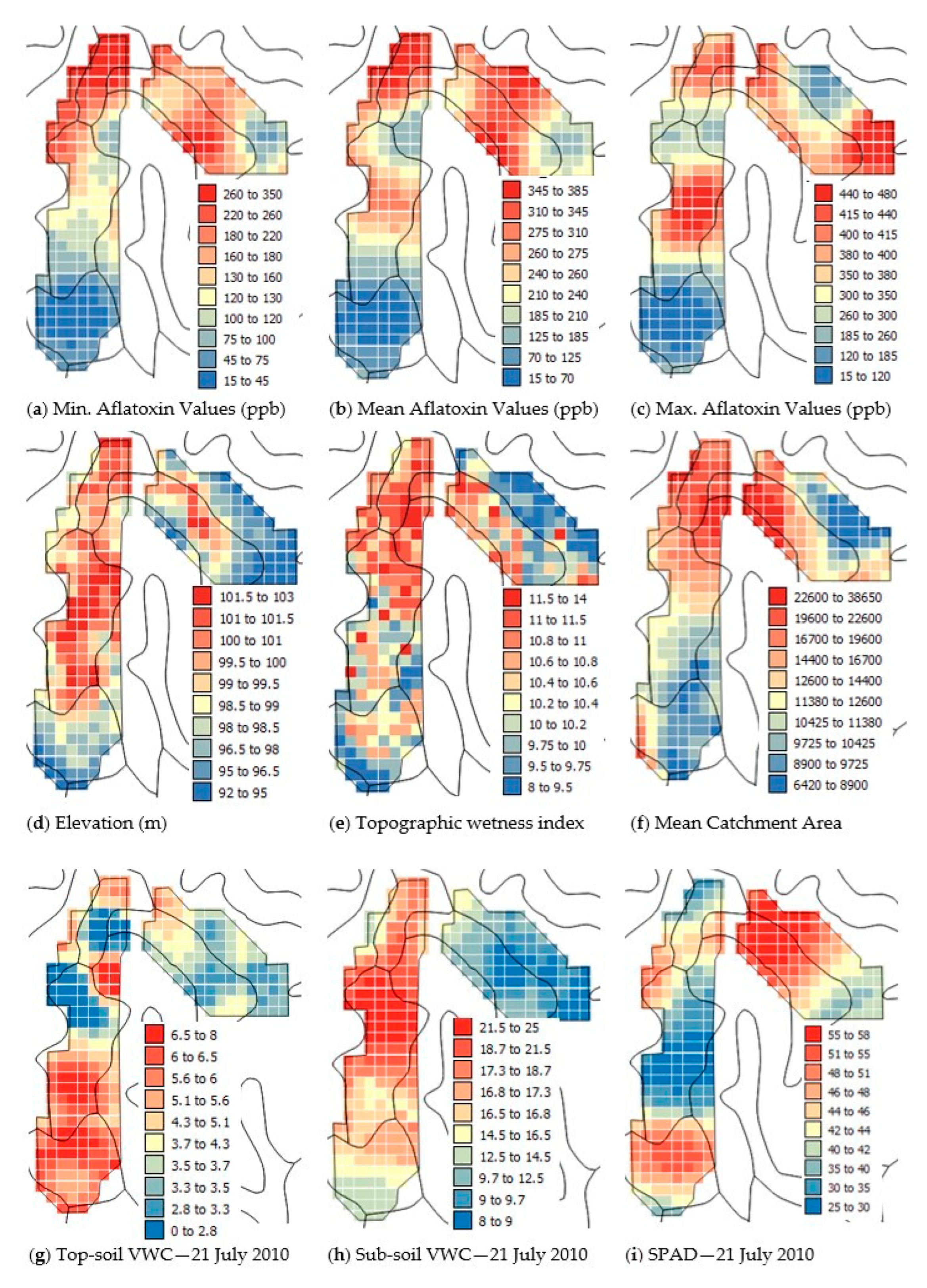
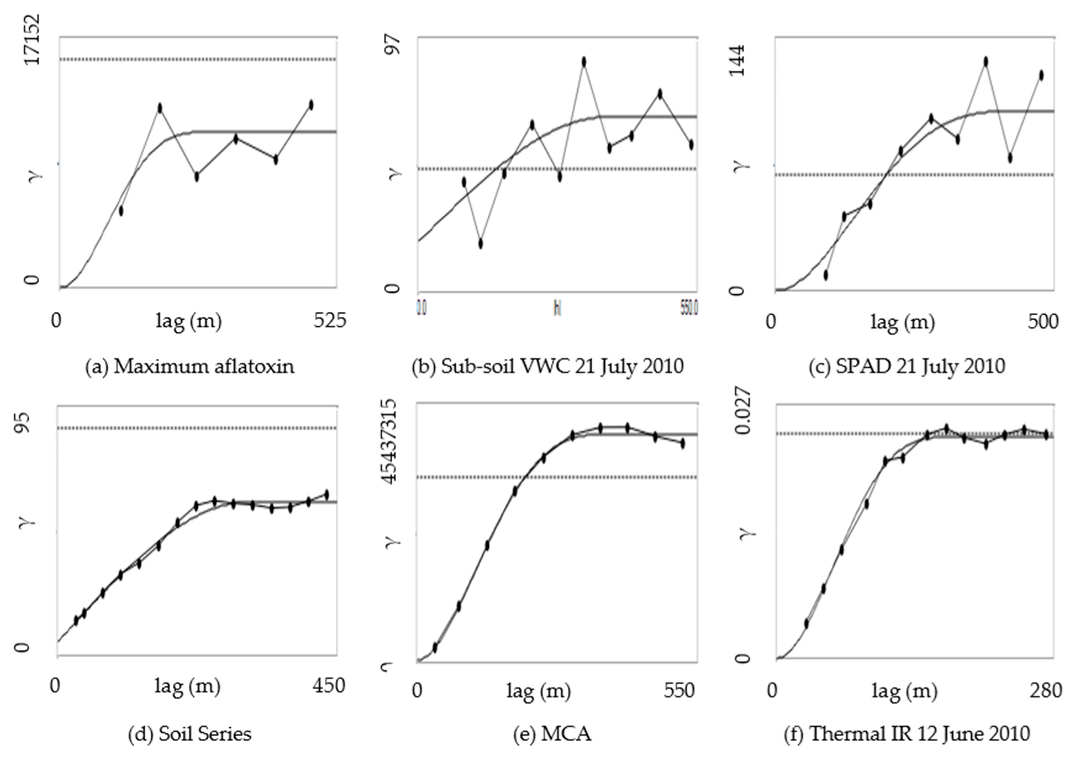
3.1. Spatial Patterns and Correlation Analysis for 2010

The results for the 2010 growing season will be analyzed first as this was when AFs samples and field observations were collected. Figure 3a shows that average MAX growing season temperatures were 2–3 °C above normal for all months (April–August) in the 2010 growing season. Figure 3b shows that precipitation totals were particularly low compared to normal in April, June and July 2010, but the rainfall was higher than normal in May and August. For the 2010 growing season as a whole, however, the rainfall was about two thirds of normal levels (Figure 3c). The rainfall for June 2010, the key mid-silk period for corn grown as a summer crop in the southern US, which has been shown to be important to AFs build-up [16,17], was about one quarter of normal levels (Figure 3b). The above normal growing season temperatures and the reduced rainfall, particularly in June 2010 make 2010 a high-risk year for AFs contamination.

Due to expense, minimal soil, crop and AFs measurements were made. Some interpolation of these values to a denser grid is necessary to see the spatial patterns in the variation of the variables. Kriging interpolation relies on having a reliable variogram to characterize the spatial variation in a property. Variograms can be erratic when based on few data [32], especially when measured on a grid or by random sampling. However, as samples were targeted within soil series with at least two samples per soil series, it is more likely that variograms may show some structure even with the small sample size. Figure 5a–c show example variograms from AFs, soil and crop variables and Figure 5d–f show example variograms from denser, freely available data from soil survey, DEM and remote sensing. The variograms for the data collected in the field are more erratic in form than those for the remotely sensed data as they are based on far fewer samples, however, they still show spatial structure with some similar variogram ranges to the variograms for remotely sensed data (

Table 2. Variogram parameters used for kriging field observation data and parameters of variograms for selected imagery data.

Variable	Model	Nugget (c0)	Sill (c1)	Range (m)
Minimum aflatoxin	Spherical	0	8175.46	194.64
Mean aflatoxin	Cubic	0	6435.14	273.37
Maximum aflatoxin	Cubic	0	10,713.10	293.61
Top-soil VWC (21 July 2010)	Cubic	0	5.93	190.86
Sub-soil VWC (21 July 2010)	Spherical	19.25	47.57	371.67
SPAD (21 July 2010)	Cubic	0	102.72	464.86
Soil series	Spherical	5.41	53.62	306.64
MCA	Cubic	0	3572.44	401.31
NDVI (12 June 2010)	Spherical	0.00014	0.0013	104.68
Thermal IR (12 June 2010)	Cubic	0	0.0237	185.08
NDVI (19 June 2010)	Spherical	0	0.0022	114.54
Thermal IR (19 June 2010)	Spherical	0	0.0070	186.02

). MIN AFs, top-soil VWC and thermal IR from two different dates all have variogram ranges of approximately 200 m. MEAN and MAX AFs and soil series have variogram ranges of approximately 300 m and sub-soil VWC, SPAD and MCA had variograms ranges of approximately 400 m. The similarity in the variogram ranges for the plant and soil variables and those from denser data made it possible to use a modified approach to kriging similar to that of Kerry and Oliver [33]; however, the variance of the data was used to determine the sill of the variogram so it was not necessary to convert the soil data to standardized z-scores before kriging. The maps resulting from this approach (Figure 4) can be seen as a reasonable spatial representation of the patterns of the variables measured in the field.

Figure 4a–c show the spatial patterns of MIN, MEAN and MAX AFs values, respectively. There are some similarities in their patterns, with all variables showing lower values for soil series 5 and some areas of soil series 31 (Table 1). For MIN and MEAN AFs, the southern portions for soil series 21 in the western field also have lower values of contamination. Series 5 has the lowest elevations so is in a receiving position hydrologically and series 21 has less light-textured soil and a clay enriched sandy clay loam (SCL) horizon that starts at just 20 cm depth. In contrast, soil series 14 and 30, tend to have the highest values of AFs (Figure 4a–c). Soil series 14 has steeper slopes (5–8%) and series 30 has a light LS texture down to 145 cm in depth and is listed as somewhat excessively drained, suggesting less available water for roots. Both soil series are also designated as not prime farmland. Soil series 31 might also be expected to have higher AFs levels given that it is designated as somewhat excessively drained, but the soil at depth in this soil series is heavier (SCL). The obvious differences in AFs levels between soil types is shown in

Table 3. Correlation and regression coefficients for Aflatoxin, field and remotely sensed data.

	Pearson Correlation			Regression
Variable	Min. Aflatoxin	Mean Aflatoxin	Max. Aflatoxin	Min. Aflatoxin		Mean Aflatoxin		Max. Aflatoxin
R2	-	-	-	0.659		0.688		0.809
				Estimate	p-Value	Estimate	p-Value	Estimate	p-Value
Intercept	-	-	-	1,514,279	0.00 *	1,752,835	0.00 *	497,332	0.00 *
MCA	0.49	0.38	0.31	NA	NA	NA	NA	0.013	0.00 *
MUSYM	0.33	0.46	0.46	−4.61	0.00 *	−5.34	0.00 *	−1.54	0.012 *
MUKEY	−0.60	−0.59	−0.52	1.14	0.002 *	3.14	0.00 *	1.46	0.0007 *
SPAD 21 July 2010	0.11	−0.07	−0.47	1.23	0.015 *	NA	NA	−10.51	0.00 *
VWC 21 July 2010	−0.56	−0.59	−0.41	−11.6	0.00 *	NA	NA	−12.82	0.00 *
logNDVI 12 June 2010	−0.01	−0.01	0.05	247	0.001 *	126.1	0.074	244.4	0.007 *
logNDVI 19 June 2010	−0.06	−0.06	−0.02	NA	NA	NA	NA	NA	NA
logNDVI 14 July 2010	−0.20	−0.13	−0.08	NA	NA	NA	NA	−615.7	0.0004 *
logNDVI 21 July 2010	−0.27	−0.17	−0.14	−333.3	0.009 *	NA	NA	NA	NA
logNDVI 30 July 2010	−0.07	−0.08	−0.21	NA	NA	NA	NA	115.07	0.1132
Thermal 12 June 2010	−0.14	−0.21	−0.18	−6.57	0.011 *	NA	NA	−20.71	0.00 *
Thermal 19 June 2010	−0.35	−0.28	0.04	−6.22	0.141	NA	NA	29.62	0.00 *
Thermal 14 July 2010	0.23	0.31	0.01	6.4	0.028 *	27.58	0.00 *	31.12	0.00 *
Thermal 21 July 2010	0.42	0.26	0.19	6.4	0.028 *	NA	NA	8.29	0.0012 *
Thermal 30 July 2010	0.30	0.27	0.27	NA	NA	14.03	0.00 *	19.67	0.00 *
logNDVI 28 May 2008	−0.70	−0.62	−0.33	-	-	-	-	-	-
logNDVI 30 May 2011	0.61	0.74	0.73	-	-	-	-	-	-
Thermal 24 June 2006	−0.54	−0.36	−0.30	-	-	-	-	-	-
Thermal 5 May 2008	0.63	0.73	0.64	-	-	-	-	-	-
Thermal 28 May 2008	−0.62	−0.63	−0.48	-	-	-	-	-	-
Thermal 25 June 2009	0.64	0.53	0.57	-	-	-	-	-	-
Thermal 30 May 2011	0.74	0.70	0.54	-	-	-	-	-	-
NDRE June 2019	−0.48	−0.65	−0.64	-	-	-	-	-	-

Correlation coefficients > 0.5 are bold, p-values with * are significant at the 0.05 level, NA means variable not included in best subset regression model—means variable not used in regression analysis.

by the relatively strong correlations between AFs values and musym, mukey, two variables that relate to soil type. Correlations are stronger for the latter and strongest with MIN AFs (r = −0.6).

As soil series delineations are heavily dependent on topography (Table 2), it is not surprising to see that elevation, TWI and MCA (Figure 4d–f) all show low values in the eastern side of the eastern field which correspond almost exactly with the boundary for soil series 31. Like MAX AFs levels, elevation values show high values throughout soil series 21 whereas MIN and MEAN AFs levels and TWI and MCA only show high values for the northern end of soil series 21. Each of these topographic variables (elevation, TWI and MCA) showed the strongest correlations with MIN AFs and weakest correlations with MAX AFs (Table 3 shows the correlations with MCA, the correlations for elevation and TWI were weaker so are not shown). Figure 4g and h show that VWC in the top- and sub-soil is lower in the eastern field, but the patterns in top-soil moisture content show greater similarity to the patterns in AFs contamination. The patterns suggest that the expected negative relationship between VWC and AFs exists, especially for the top-soil. The strongest negative correlation (r = −0.59) with top-soil VWC was for MEAN AFs levels (Table 3). Correlations with sub-soil VWC were weaker so were not included. Finally, SPAD measurements showed almost the reverse patterns of variation to MAX AFs levels (compare Figure 4c,i). The correlations in Table 3 confirmed this observation with the strongest negative relationship between SPAD and AFs being for the MAX values (r = −0.47). A negative correlation between SPAD and AFs would be expected with less green (less healthy) plants having higher AFs levels.

3.2. Regression Analysis for 2010 Growing Season

Following correlation analysis best sub-set regression was performed using the most strongly correlated field data and NDVI and thermal IR data from imagery for dates in June and July 2010. Three regressions were performed with MIN, MEAN and MAX AFs values as the dependent variables. Table 3 shows that the R² value for regression was highest for MAX AFs (R² = 0.809) and least for MIN AFs (R² = 0.659). All field variables were included in the MAX AFs regression, as well as all but two NDVI variables. Similarly, many variables were included in the MIN AFs regression, but the MEAN AFs regression only included soil series, NDVI from 12 June 2010 and thermal IR from 14 July 2010 and 30 July 2010. NDVI from 12 June 2010 was included in all three regressions but the estimates were positive in each case rather than negative as might be expected. There were low values of NDVI in this image for soil series 5, 14 and 30. Knowing the spatial patterns of soil moisture (Figure 4g), this suggests that a factor other than water may have been limiting crop greenness for soil series 5 as this point in time. Table 1 shows that soil series 5 is not considered prime farmland but does not state the reasons why. Based on the regression analysis, there were two distinct groups of points in the observed vs. predicted scatter plots (not shown). These largely corresponded with a low-risk zone for soil series 5 and a high-risk zone for all other soil series.

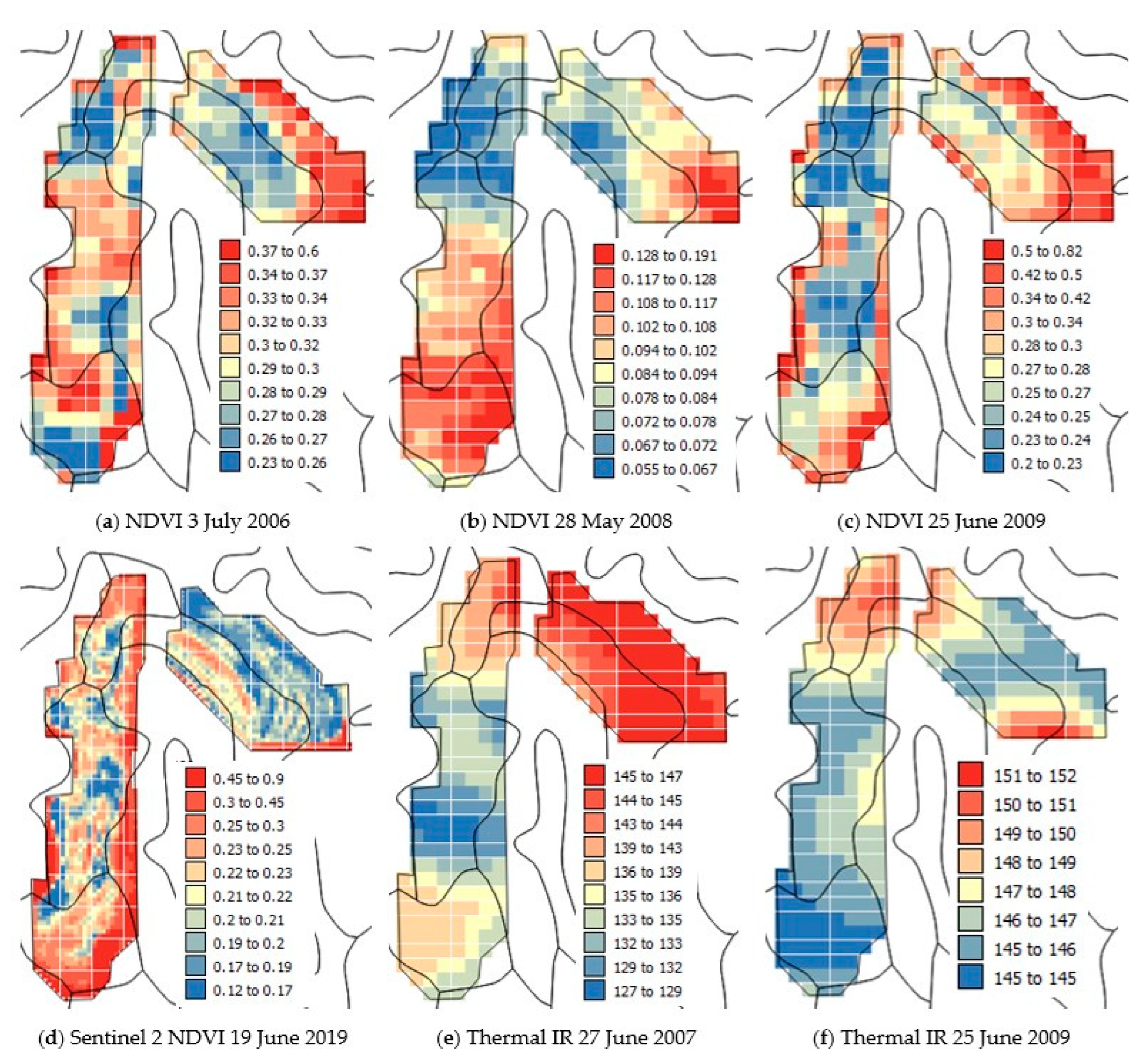
3.3. Imagery Data for the 2006–2011 and 2019 Growing Seasons

Following the development of 2 risk zones for 2010 based on regression, imagery data for other years was analyzed in relation to the patterns of AFs contamination for 2010. Figure 6 shows some NDVI and thermal IR data for the field site for different years and months. There are some similarities in the distribution of values between months and years. Soil series 14 and 30 (Figure 2 and Table 1) tend to show low values of NDVI and higher values of thermal IR. These are the soil series which also had the highest AFs levels (Figure 4a–c). AFs levels have been shown to be greatest in locations that have a combination of drought and high temperatures. It seems that NDVI patterns are reflecting lack of water (see Figure 4g) and thermal IR is reflecting patterns of high temperatures, as might be expected. Where both of these conditions coincide, the AFs values are greatest. Table 3 shows that in most cases NDVI is negatively correlated with AFs variables and AFs are positively correlated with thermal IR. While 2019 NDRE and NDVI were well-correlated with AFs (Table 3 and Figure 6d) there did not seem to be a major advantage to the greater spatial and spectral resolution provided by these data. Indeed, the greater spatial resolution shown in the 2019 NDVI data would result in smaller less consistent risk zones being determined.

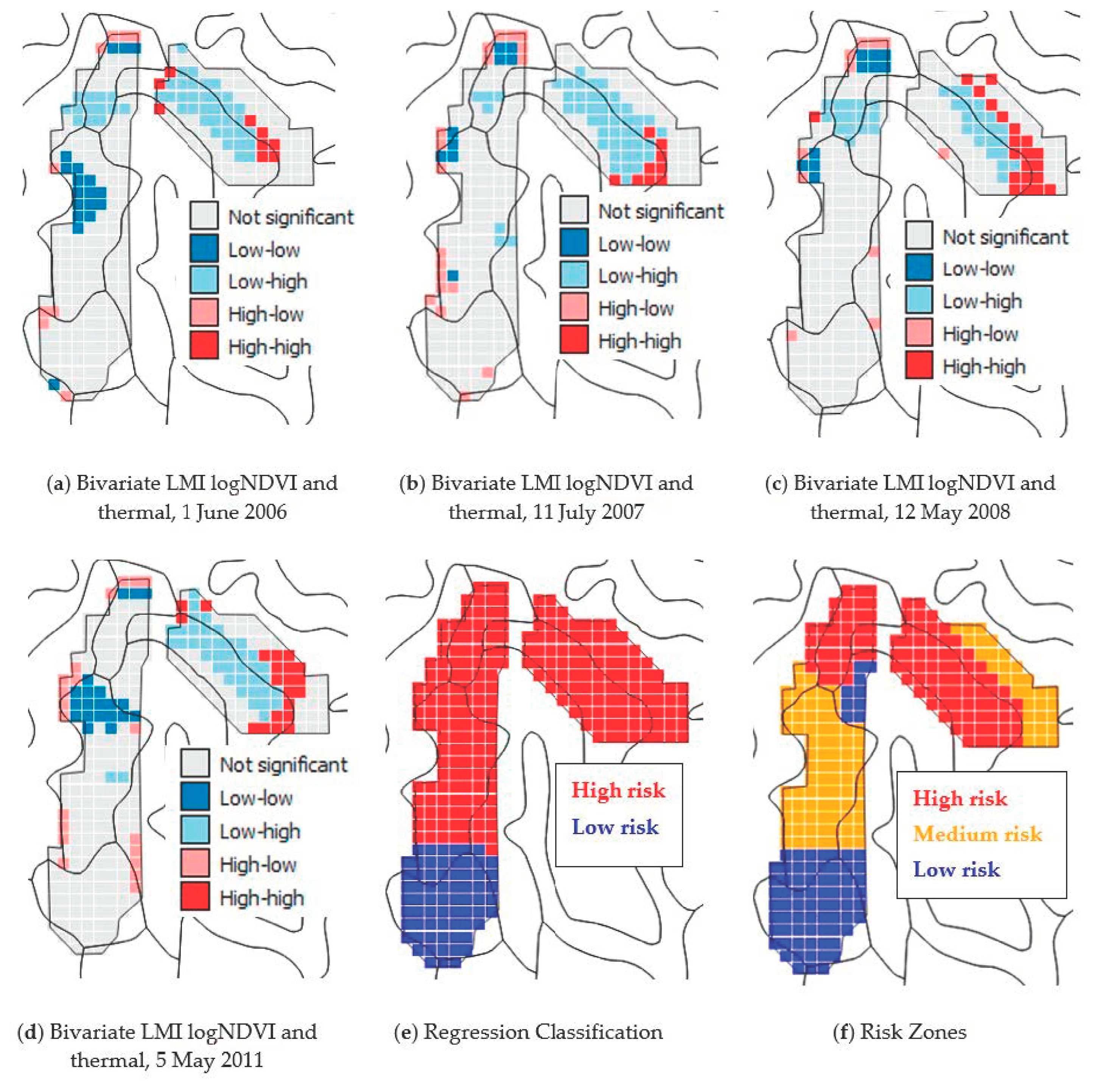
3.4. Local Moran’s I Analysis

Figure 7a–d shows pixel maps for bivariate LMI between log¹⁰ NDVI and thermal IR data for some dates. Each shows a significant (p = 0.05) cluster of low-high points that corresponds with soil series 14 and 30 and this was also common on other dates. This means that these clusters have significantly lower NDVI values and significantly higher thermal IR values than their neighbors. These two soil series both have westerly aspects, whereas series 31 in the eastern side of both fields faces north to north-east. Westerly aspects receive direct sunlight at hotter times of the day than north and north-easterly facing slopes which would lead to greater evapotranspiration and therefore drought in the areas that face west.

Figure 7f shows a risk zone map with 3 zones developed from a combination of the two zones from regression (Figure 7e) and the definition of the highest risk zone defined by soil series 14 and 30 identified with LMI. Kruskal–Wallis H tests were used to compare the differences in AFs (

Table 4. Summary of Kruskal–Wallis H tests to determine the best method for defining aflatoxin risk zones and Pearson correlations between PC1 and PC2 and the aflatoxin variables.

	Kruskal–Wallis H Test Statistic Values				Pearson Correlation
	Regression and LMI	PC1	PC2	PC1 and PC2	PC1	PC2
Minimum aflatoxin	150.9	74.5	137.8	172.1	0.54	0.71
Mean aflatoxin	192.3	68.5	138.3	167.6	0.55	0.72
Maximum aflatoxin	204.8	25.5	113.5	125.9	0.39	0.65

p-value for all tests < 0.0001.

, first column). The p-value for all three tests was <0.0001 and the mean rank values of AFs in each class showed the expected order in terms of magnitude that one would expect for high, medium and low risk zones, respectively. The values of the H statistic, however, show that the classification of zones using the combination of regression and the bi-variate LMI is best for MAX AFs levels. Other Kruskal–Wallis H tests (results not shown) also showed that risk zones represented expected significant (p < 0.05) differences in top-soil VWC and 75% of the imagery data. Differences between zones were less significant for April imagery and months with less drought (Figure 3).

3.5. K-Means Classification of Imagery

Imagery from a range of months and years was used to develop two-class K-means classifications using standardized data for NDVI and thermal IR. Two-class K-means classifications were also developed for MIN, MEAN and MAX AFs values and the Kappa statistic was computed to compare classifications and percent agreement between classifications was calculated (

Table 5. Kappa statistic and percent agreement results for comparison of K-means classifications based on kriged minimum, mean and maximum aflatoxin values and imagery (NDVI and Thermal IR) from various months in 2006–2011.

Variable or Imagery Date	Minimum Aflatoxin			Mean Aflatoxin			Maximum Aflatoxin
	Kappa Statistic	p-Value	% Agreement	Kappa Statistic	p-Value	% Agreement	Kappa Statistic	p-Value	% Agreement
5 April 2006	0.059	0.26	50.7	−1.330	0.021	48.6	−0.067	0.250	51.0
24 June 2006	0.184	0.001	61.8	−0.205	0	55.1	0.213	0	56.1
27 June 2007	0.530	0	77.0	0.431	0	70.3	0.343	0	65.9
28 May 2008	0.402	0	67.6	0.661	0	85.8	0.410	0	74.7
8 July 2008	0.024	0.474	44.3	−0.070	0.157	61.1	−0.100	0.037	58.1
25 June 2009	0.313	0	73.3	0.298	0	50.4	0.327	0	53.4
2 July 2009	0.223	0	59.4	0.115	0.045	59.4	0.133	0.022	59.8
9 April 2010	−0.044	0.419	45.9	−0.147	0.01	46.6	−0.129	0.025	46.9
12 June 2010	0.023	0.063	42.2	0.071	0.001	69.9	0.064	0.002	67.6
19 June 2010	0.049	0.401	51.7	0.138	0.009	58.4	0.083	0.124	55.4
14 July 2010	0.169	0.002	56.8	0.076	0.187	57.4	0.050	0.391	55.7
21 July 2010	0.404	0	70.3	0.220	0.000	60.8	0.172	0.002	58.4
30 July 2010	0.138	0.002	52.7	0.102	0.074	63.5	0.136	0.016	63.9
30 May 2011	0.563	0	83.0	0.521	0	85.8	0.416	0	78.7
6 June 2011	0.049	0.189	46.3	0.163	0.002	68.6	0.103	0.045	64.9
15 June 2011	−0.014	0.699	42.6	0.091	0.078	66.2	0.087	0.086	64.5

). Scree plots (not shown) for K-means classifications of the three AFs variables with different numbers of classes suggested that classifications with 3–4 classes would be most appropriate for the AFs data, however, comparisons between two-class classifications were investigated to represent a simplified case. Kappa values tended to be largest and most significant (p < 0.05) when there were larger percentage agreements in the two-class classifications based on AFs levels and those for the imagery data. The Kappa statistic values, however, take into account whether the percentage agreement was likely to occur by chance so there are some moderate agreements in Table 5 which have low Kappa values because they were more likely to occur due to chance.

For MIN AFs, the greatest percentage agreements were with imagery from 30 May 2011, 27 June 2007, 25 June 2009, 21 July 2010, 28 May 2008 and 28 June 2006. Each of the months associated with these images had markedly less than their normal monthly precipitation (Figure 3b) and each of these years apart from 2009 had markedly less precipitation than normal throughout the growing season (Figure 3c). Furthermore, each of these months, apart from May 2008, had higher than normal monthly Tmax values. For the two-class MEAN AFs classification the imagery-based classification for seven months showed percentage agreements > 60% and three of these months were the same months as showed the highest percentage agreement with MIN AFs values (Table 5). The highest percentage agreements (both 85.8%) were for 28 May 2008 and 30 May 2011, respectively. The former of these dates also showed the highest Kappa value in Table 5. Both of these months showed precipitation levels that were about one fifth of their normal levels (Figure 3b) and temperatures were around normal in May 2008, but a couple of degrees above normal in May 2011 (Figure 3a). The two-class MAX AFs classification and the imagery-based classifications showed percentage agreements > 60% for the same seven months as the MEAN AFs classification. The highest percentage agreements (74.7 and 78.7%) were for the same dates as those in the MEAN AFs classification, 28 May 2008 and 30 May 2011, respectively. These results seem to suggest that imagery-based classifications are more sensitive to drought early rather than late in the growing season. The similarity in the dates with the greatest percent agreements between classifications for MEAN and MAX AFs suggests that imagery is better at reflecting differences in these variables than MIN AFs. This is desirable as farmers want to manage for MEAN or MAX AFs levels.

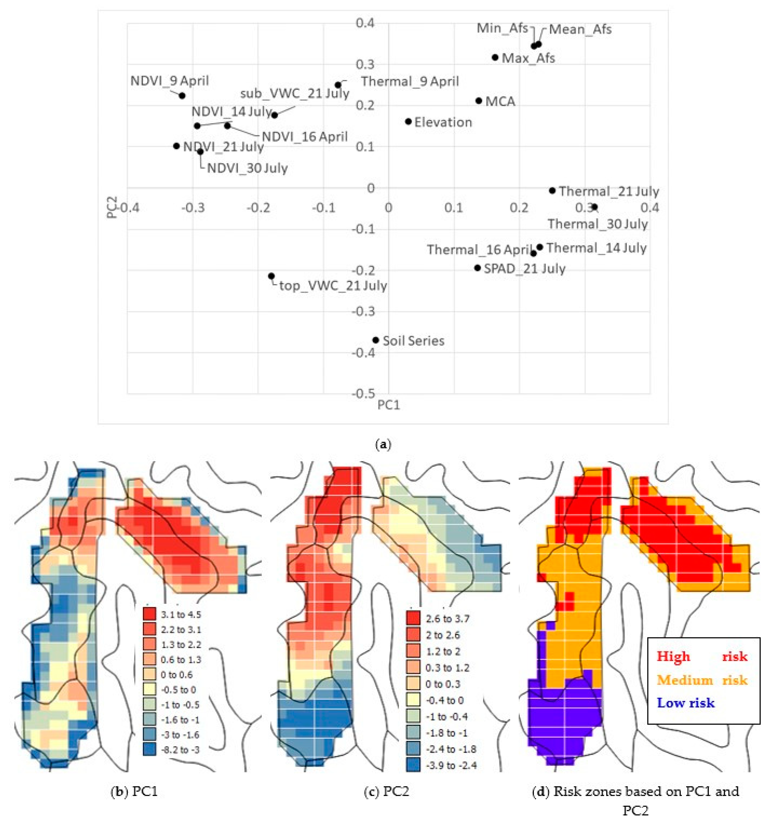
3.6. Principal Components Analysis

Principal components (PC) analysis was used to gain greater understanding of the correlation between field and remotely sensed variables for 2010 and to identify the locations that were most similar in a multi-variate sense. A total of 20 variables with values at 296 locations on a 30 m grid were used for PCA. PC1 and PC2 accounted for variation equivalent to 29% and 22% of the variation in the original dataset, respectively. Figure 8a plots the variables used in terms of PC1 and PC2. The AFs measurements plot in the top right quadrant of the graph along with MCA and elevation, but MCA plots closer to AFs values showing a stronger positive relation to them. Top-soil VWC and soil series plot in the bottom left quadrant being the greatest distance from the AFs values and suggesting the strongest negative relationship with AFs. NDVI for all dates plots in the top left quadrant along with sub-soil VWC. The NDVI values also show a negative correlation with AFs. All thermal IR variables plot in the lower right quadrant along with SPAD measurements, apart from the thermal IR values for 9 April 2010. The thermal IR variables show a negative association with AFs values in terms of PC2.

Figure 8b and c show the PC1 and PC2 scores of each of the 296 sampling points. There are higher values of PC1 for soil series 14 and 30 (Figure 2 and Table 1). For PC2, the values are lowest for soil series 5 and 31 and highest for soil series 14 and 21 (Figure 2 and Table 1). Three-class classifications were developed for PC1, PC2 and both PCs based on natural classes in the PC histograms. Figure 8d shows the classification based on both PCs. It is very similar to the classification based on the regression and LMI results but most of the eastern field is identified as high risk rather than just soil series 30. Table 4 shows the Kruskal–Wallis H test results when MIN, MEAN and MAX AFs values are compared between zones developed using PC1, PC2 and both PCs. All tests showed highly significant (p < 0.0001) differences which showed the expected order of values relating to risk, so the best classification approach had to be judged based on the H statistic values. These were higher for PC2 than PC1 and highest for PC1 and PC2 together suggesting that information from more variables rather than fewer is desirable in defining risk zones. Pearson correlation values showed that PC2 was actually more strongly correlated with AFs values than PC1. The Kruskal–Wallis H test results (Table 4) show that overall, the best approach for defining management zones for MAX and MEAN AFs was the combined regression and LMI approach. However, for MIN AFs, the two PCs approach was the best.

Based on the 2010 AFs values shown in Figure 4a–c, all values would exceed the FDA 20 ppb limit and most areas would also exceed the 100 ppb limit. The only area that would not exceed the 100 ppb limit would be soil series 5 which was identified as the low risk zone by regression and the both PCs classification. Therefore, in high-risk years this soil series could be harvested separately to avoid all grain being rejected for more general animal consumption. Figure 4b shows that there are some quite large areas corresponding largely with the medium risk zones (Figure 7f and Figure 8d) where the mean concentrations are less than 300 ppb so the grain from these areas could be used for mature finishing beef cattle [10]. Based on Figure 4b, it is likely that in high-risk years like 2010, only the grain from the highest risk zone (Figure 7f and Figure 8d) would need to be completely rejected. This shows the importance of harvesting the different risk zones separately and storing the grain as micro-batches so that the whole crop is not rejected. It also suggests that, if mitigation strategies, like irrigation or pesticide application, were employed in the highest risk zone, the grain from this zone may not need to be rejected in high-risk years.

Data on the spatial variation of AFs values within these fields from a low-risk year where RF is higher than normal and TMax is lower than normal are needed to determine what are the best strategies for AFs mitigation in this field. If the AFs values are above FDA thresholds for soil series 14 and 31 even in low-risk years then the farmer should consider not growing corn in these fields, or planting more resistant varieties at lower densities in the soil series most at risk of contamination. They should also consider installing irrigation infrastructure and soil moisture sensors in each risk zone so that the crop does not experience drought. One would expect the values of AFs to be generally lower in low-risk years, so in these years it would be useful to harvest and store the grain separately from the three zones identified by the regression and LMI approach rather than just two zones to maximize the potential income from corn sold for different uses.

4. Conclusions

This work investigated the spatial variation in key variables that can indicate drought status within a field to identify zones with different risk of AFs contamination in a cost-effective manner for a high-risk year (2010). Correlations between expensive and time-consuming measurements of AFs and field observations and free data namely: topography, soil type, and NDVI and thermal IR for 2010 showed the expected signs and relative strengths. Regression and PCA analysis showed the importance of soil series and top-soil VWC to AFs values. The former identified a soil series (5) with lower AFs values than others. This allowed the development of AFs risk zones which showed highly significant differences in AFs level. This showed that drought status at the field scale is important to AFs contamination just as previous research has shown it is important at the county and within county scale.

When remotely sensed data for other years was considered to determine if zones were likely to be consistent in time, bi-variate LMI analysis consistently identified clusters of significantly lower NDVI and higher thermal IR values for two soil series (14 and 30). Correlation analysis and comparison of K-means classifications of imagery from different months and years showed the largest correlations and percent agreements when precipitation was markedly lower and Tmax higher than normal, namely when drought was strongest. This was particularly the case when drought occurred early in the growing season (April or May).

As suspected, the main drivers of drought within fields relate to soil type/texture and topography. While weather determines if a year is low or high risk and was most important at the county scale in previous studies (ie June TMax and June RF), it does not vary markedly within fields. This work has shown that within a given season, NDVI and thermal IR from imagery are most indicative of the spatial variation of drought conditions within a field when the monthly weather conditions are droughty. As suspected, the temporal analysis of the imagery data suggests that AFs risk zones seem somewhat stable in time and farmers could potentially identify these risk zones using only free imagery, weather, topography and soil series information. Imagery from several dates is needed to identify patterns in relation to weather conditions and soil series and farmers should select imagery from the most droughty growing season months in the past. Once established, farmers can at the very least, harvest and store grain from the different risk zones separately. However, it may be prudent for fields like those in this study, where levels are generally above the two more general use FDA thresholds, to install soil moisture sensors and variable rate irrigation infrastructure so that water can be applied to relieve drought in the higher risk zones and whole batches or even several separated micro-batches of grain are not rejected or can only be used for very specific purposes and thus generate less income.

References

1. Patriarca, A.; Medina, A.; Pinto, V.F.; Magan, N. Temperature and water stress impacts on growth and production of altetoxin-II by strains of Alternaria tenuissima from Argentinean wheat. World Mycotoxin J. 2014, 7, 329–334. [Google Scholar] [CrossRef]
2. Payne, G.A. Aflatoxin in maize. CRC Crit. Rev. Plant Sci. 1992, 10, 423–440. [Google Scholar] [CrossRef]
3. Wilson, J.P.; Hanna, W.W.; Wilson, D.M.; Beaver, R.W.; Casper, H.H. Fungal and mycotoxin contamination of pearl-millet grain in response to environmental conditions in Georgia. Plant Dis. 1993, 77, 121–124. [Google Scholar] [CrossRef]
4. Abbas, H.K.; Weaver, M.A.; Zablotowicz, R.M.; Horn, B.W.; Shier, W.T. Relationships between aflatoxin production and sclerotia formation among isolates of Aspergillus section Flavi from the Mississippi Delta. Eur. J. Plant Pathol. 2005, 112, 283–287. [Google Scholar] [CrossRef]
5. Adegoke, G.O.; Otumu, E.J.; Akanni, A.O. Influence of grain quality, heat, and processing time on the reduction of aflatoxin b-1 levels in tuwo and ogi—2 cereal-based products. Plant Foods Hum. Nutr. 1994, 45, 113–117. [Google Scholar] [CrossRef] [PubMed]
6. Barrett, J.R. Liver cancer and aflatoxin: New information from the Kenyan outbreak. Environ. Health Persp. 2005, 113, A837–A838. [Google Scholar] [CrossRef] [Green Version]
7. FDA. Bad Bug Book, Foodborne Pathogenic Microorganisms and Natural Toxins, 2nd ed.; Food and Drug Administration: Laurel, MD, USA, 2012. Available online: http://www.fda.gov/downloads/Food/FoodborneIllnessContaminants/UCM297627.pdf (accessed on 12 October 2022).
8. FDA. Sec. 683.100 Action Levels for Aflatoxins in Animal Food Compliance Policy Guide. Guidance for FDA Staff; FDA: Rockville, MD, USA, 2019.
9. EU. Commission Regulation (EC) No 1881/2006 of 19 December 2006 Setting Maximum Levels for Certain Contaminants in Foodstuffs; EU: Maastricht, The Netherlands, 2006. [Google Scholar]
10. Liu, Y.; Wu, F. Global burden of aflatoxin-induced hepatocellular carcinoma: A risk assessment. Environ. Health Perspect. 2010, 118, 818–824. [Google Scholar] [CrossRef] [PubMed] [Green Version]
11. FDA. Available online: http://www.fda.gov/ICECI/ComplianceManuals/CompliancePolicyGuidanceManual/ucm074703.htm (accessed on 18 August 2022).
12. Papadoyannis, I.N. HPLC in Clinical Chemistry (Chromatographic Science Series), 1st ed.; Marcel Dekker: New York, NY, USA, 2008; p. 504. [Google Scholar]
13. EU. Commission Regulation (EC) No 401/2006 of 23 February 2006 Laying Down the Methods of Sampling and Analysis for the Official Control of the Levels of Mycotoxins in Foodstuffs. 2006. Available online: https://eur-lex.europa.eu/legal-content/EN/ALL/?uri=CELEX%3A32006R0401 (accessed on 14 August 2022).
14. Maestroni, B.; Cannavan, A. Sampling Strategies to Control Mycotoxins, Joint FAO/IAEA Division of Nuclear Techniques in Food and Agriculture; International Atomic Energy Agency (IAEA): Vienna, Austria, 2011. [Google Scholar]
15. Horn, B.W.; Sorensen, R.B.; Lamb, M.C.; Sobolev, V.S.; Olarte, R.A.; Worthington, C.J.; Carbone, I. Sexual reproduction in Aspergillus flavus sclerotia naturally produced in corn. Phytopathology 2014, 104, 75–85. [Google Scholar] [CrossRef] [PubMed] [Green Version]
16. Brenneman, T.B.; Wilson, D.M.; Beaver, R.W. Effects of diniconazole on Aspergillus populations and aflatoxin formation in peanut under irrigated and non-irrigated conditions. Plant Dis. 1993, 77, 608–612. [Google Scholar] [CrossRef]
17. Salvacion, A.; Ortiz, B.V.; Scully, B.; Wilson, D.M.; Hoogenboom, G.; Lee, D. Effect of rainfall and maximum temperature on corn aflatoxin in the Southeastern U.S. coastal plain. In Proceedings of the Climate Information for Managing Risks, Orlando, FA, USA, 24–27 May 2011. [Google Scholar]
18. Kerry, R.; Ortiz, B.V.; Ingram, B.R.; Scully, B.T. A Spatio-Temporal investigation of risk factors for aflatoxin contamination of corn in southern Georgia, USA using geostatistical methods. Crop Prot. 2017, 94, 144–158. [Google Scholar] [CrossRef]
19. Yoo, E.; Kerry, R.; Ingram, B.R.; Ortiz, B.; Scully, B. Defining and Characterizing Aflatoxin Contamination Risk Areas for Corn in Georgia, USA: Adjusting for Collinearity and Spatial Correlation. Spat. Stat. 2018, 28, 84–104. [Google Scholar] [CrossRef] [Green Version]
20. Battilani, P.; Toscano, P.; Van der Fels-Klerx, H.J.; Moretti, A.; Camardo Leggieri, M.; Brera, C.; Rortais, A.; Goumperis, T.; Robinson, T. Aflatoxin B1 contamination in maize in Europe increases due to climate change. Sci. Rep. 2016, 6, 24328. [Google Scholar] [CrossRef] [PubMed] [Green Version]
21. Kerry, R.; Ingram, B.; Garcia-Cela, E.; Magan, N.; Ortiz, B.V.; Scully, B. Determining Future aflatoxin contamination risk scenarios for corn in Southern Georgia, USA using spatio-temporal modelling and future climate simulations. Sci. Rep. 2021, 11, 13522. [Google Scholar] [CrossRef]
22. Hell, K.; Cardwell, K.F.; Setamou, M.; Schulthess, F. Influence of insect infestation on aflatoxin contamination of stored maize in four agroecological regions in Benin. Entomol. Afr. Entomol. 2000, 8, 169–177. [Google Scholar]
23. Liu, N.; Liu, C.; Dudaš, T.N.; Loc, M.Č.; Bagi, F.F.; Van der Fels-Klerx, H.J. Improved aflatoxins and fumonisins forecasting models for maize (PREMA and PREFUM), using combined mechanistic and Bayesian Network modeling—Serbia as a case study. Front. Microbiol. 2021, 12, 643604. [Google Scholar] [CrossRef] [PubMed]
24. Palumbo, J.D.; O’Keeffe, T.L.; Kattan, A.; Abbas, H.K.; Johnson, B.J. Inhibition of aspergillus flavus in soil by antagonistic pseudomonas strains reduces the potential for airborne spore dispersal. Phytopathology 2010, 100, 532–538. [Google Scholar] [CrossRef] [PubMed] [Green Version]
25. Damianidis, D.; Ortiz, B.; Windham, G.; Scully, B.; Woli, P. Predicting pre-harvest Aflatoxin corn contamination risk with a rought index. In Precision Agriculture’15; Wageningen Academic Publishers: Wageningen, The Netherlands, 2015; pp. 788–809. [Google Scholar]
26. Hatfield, J.L.; Prueger, J.H. Value of using different vegetative indices to quantify agricultural crop characteristics at different growth stages under varying management practices. Remote Sens. 2010, 2, 562–578. [Google Scholar] [CrossRef] [Green Version]
27. Wang, R.; Cherkauer, K.; Bowling, L. Corn response to climate stress detected with satellite-based NDVI time series. Remote Sens. 2016, 8, 269. [Google Scholar] [CrossRef] [Green Version]
28. Jones, H.G.; Serraj, R.; Loveys, B.R.; Xiong, L.; Wheaton, A.; Price, A.H. Thermal infrared imaging of crop canopies for the remote diagnosis and quantification of plant responses to water stress in the field. Funct. Plant Biol. 2009, 36, 978–989. [Google Scholar] [CrossRef] [Green Version]
29. Sepúlveda-Reyes, D.; Ingram, B.; Bardeen, M.; Zúñiga, M.; Ortega-Farías, S.; Poblete-Echeverría, C. Selecting canopy zones and thresholding approaches to assess grapevine water status by using aerial and ground-based thermal imaging. Remote Sens. 2016, 8, 822. [Google Scholar] [CrossRef] [Green Version]
30. Kerry, R.; Ingram, B.; Orellana, M.; Ortiz, B.V.; Scully, B.T. Development of a method to assess the risk of aflatoxin contamination of corn within counties in southern Georgia, USA using remotely sensed data. Smart Agric. Technol. 2022, 3, 100124. [Google Scholar] [CrossRef]
31. Jaime-Garcia, R.; Cotty, P.J. Aflatoxin contamination of commercial cottonseed in south Texas. Phytopathology 2003, 93, 1190–1200. [Google Scholar] [CrossRef] [PubMed] [Green Version]
32. Damianidis, D.; Ortiz, B.V.; Bowen, K.L.; Windham, G.L.; Hoogenboom, G.; Hagan, A.; Knappenberger, T.; Abbas, H.K.; Scully, B.T.; Mourtzinis, S. Minimum Temperature, Rainfall, and Agronomic Management Impacts on Corn Grain Aflatoxin Contamination. Agron. Soils Environ. Qual. 2018, 110, 1697–1708. [Google Scholar] [CrossRef] [Green Version]
33. Xiong, D.; Chen, J.; Yu, T.; Gao, W.; Ling, X.; Li, Y.; Peng, S.; Huang, J. SPAD-based leaf nitrogen estimation is impacted by environmental factors and crop leaf characteristics. Sci. Rep.-UK. 2015, 5, 13389. [Google Scholar] [CrossRef] [Green Version]
34. Bista, D.R.; Heckathorn, S.A.; Jayawardena, D.M.; Mishra, S.; Boldt, J.K. Effects of Drought on Nutrient Uptake and the Levels of Nutrient-Uptake Proteins in Roots of Drought-Sensitive and -Tolerant Grasses. Plants 2018, 7, 28. [Google Scholar] [CrossRef] [Green Version]
35. Tadono, T.; Ishida, H.; Oda, F.; Naito, S.; Minakawa, K.; Iwamoto, H. Precise Global DEM Generation by ALOS PRISM, ISPRS. J. Photogramm. Remote Sens. 2014, 2, 71–76. [Google Scholar]
36. Boehner, J.; Selige, T. Spatial prediction of soil attributes using terrain analysis and climate regionalisation. In SAGA-Analyses and Modelling Applications; Boehner, J., McCloy, K.R., Strobl, J., Eds.; Goettinger Geographische Abhandlungen: Goettingen, Germany, 2006; pp. 13–28. [Google Scholar]
37. Beven, K.J.; Kirkby, M.J. A physically based, variable contributing area model of basin hydrology/Un modèle à base physique de zone d’appel variable de l’hydrologie du bassin versant. Hydrol. Sci. J. 1979, 24, 43–69. [Google Scholar] [CrossRef] [Green Version]
38. Conrad, O.; Bechtel, B.; Bock, M.; Dietrich, H.; Fischer, E.; Gerlitz, L.; Wehberg, J.; Wichmann, V.; Böhner, J. System for Automated Geoscientific Analyses (SAGA) v. 2.1.4. Geosci. Model Dev. 2015, 8, 1991–2007. [Google Scholar] [CrossRef] [Green Version]
39. Webster, R.; Oliver, M.A. Sample adequately to estimate variograms of soil properties. J. Soil Sci. 1992, 43, 177–192. [Google Scholar] [CrossRef]
40. Kerry, R.; Oliver, M.A. Determining nugget: Sill ratios of standardized variograms from aerial photographs to krige sparse soil data. Precis. Agric. 2008, 9, 33–56. [Google Scholar] [CrossRef]
41. Jacquez, G.M.; Goovaerts, P.; Kaufmann, A.; Rommel, R. SpaceStat 4.0 User Manual: Software for the Space-Time Analysis of Dynamic Complex Systems, 4th ed.; BioMedware: Ann Arbor, MI, USA, 2014. [Google Scholar]
42. IBM Corp. IBM SPSS Statistics for Windows, Version 25.0; IBM Corp: Armonk, NY, USA, 2017. [Google Scholar]
Figure 1. Location map showing location of the field site (star) (31.53° N and 85.87° W) and Enterprise, AL, weather station (circle) (31.33° N 85.85° W).
Agronomy 12 02524 g001
Figure 2. Map (a) showing field observation locations (red dots), field boundaries (black lines) and soil series (colors). (b) Aerial photo showing soil series boundaries (orange lines) and numbers, details of soil series based on numbers in https://websoilsurvey.nrcs.usda.gov/app/WebSoilSurvey.aspx (accessed on 14 August 2022) given in Table 1.
Agronomy 12 02524 g002
Figure 3. Graphs showing normal and growing season (April–August) (a) maximum temperatures (Tmax, °C) (accuracy ± 2 °C), (b) monthly precipitation (mm) (±50 mm) and (c) growing season precipitation (mm) for Enterprise, AL in 2005–2011.
Agronomy 12 02524 g003
Figure 4. Pixel maps (30 m) of (a) minimum, (b) mean and (c) maximum kriged aflatoxin, (d) elevation, (e) topographic wetness index, (f) mean catchment area, (g) Top-soil VWC for 21 July 2010, (h) Sub-soil VWC for 21 July 2010 and (i) crop SPAD measurements for 21 July 2010. Black lines show soil series boundaries.
Agronomy 12 02524 g004
Figure 5. Sample variograms for (af).
Agronomy 12 02524 g005
Figure 6. Pixel maps (30 m) of NDVI (ad) and thermal IR (ef) from LandSat (ac,ef) and Sentinel 2 (d) imagery on selected dates. Black lines show soil series boundaries.
Agronomy 12 02524 g006
Figure 7. Pixel maps (30 m) of bivariate local Moran’s I (LMI) of NDVI and Thermal IR (ad) and risk zones based on two (e) or three (f) classes. Black lines show soil series boundaries.
Agronomy 12 02524 g007
Figure 8. (a) PCA plot of 2010 soil and remotely sensed variables in terms of PC1 and PC2 which account for 51% of variation in the data set. Plots of PC1 (b) and PC2 scores (c) on a 30 m grid and (d) a classification based on soil and sensed data for 2010. Black lines show soil series boundaries.
Agronomy 12 02524 g008