Offshore Spreading of a Supercritical Plume Under Upwelling Wind Forcing: A Case Study of the Winyah Bay Outflow

Introduction

Estuarine buoyant outflows are frequently modulated by tides, and run off on the continental shelf as energetic ebbing currents, sometimes further amplified by natural or artificial lateral constraints (e.g., jetties) at the mouth. Upon entering the shelf, the buoyant discharge detaches from the sloping bottom (a lift-off zone) and spreads laterally as a thin buoyant layer (e.g., Wright and Coleman, 1971; Garvine, 1974; MacDonald and Geyer, 2005; Branch et al., 2020). The lift-off renders the buoyant layer supercritical, that is, F_i > 1, where $F_i=U_s/\sqrt{g^{\prime }h}$ is the internal Froude number, U_s is the surface velocity, h is the buoyant layer thickness, g′ = g△ρ/ρ₀ is the reduced gravity, g is the acceleration due to gravity, Δρ is the buoyant layer density anomaly, and ρ₀ is the ambient seawater density. The lift-off depth depends on the flow characteristics in the estuarine channel and is inversely proportional to the outflow Froude number (where flow characteristics are taken at the mouth; e.g., Atkinson, 1993; Wang et al., 2015). Supercritical outflows undergo rapid lateral spreading, vigorous entrainment, and mixing until the buoyant layer transitions into subcritical regime (e.g., Hetland, 2005, 2010). After that, circulation in the plume is shaped by the Earth’s rotation, leading to the formation of an anticyclonic bulge. Newly discharged water can recirculate around the bulge multiple times (feeding its growth) or can exit it and continue along the coast as a coastal buoyancy driven current (also referred to as a far field plume; e.g., Fong and Geyer, 2002; Horner-Devine et al., 2009). The natural propagation of the coastal current is in the direction of a Kelvin wave propagation (hereinafter referred to as downstream), but it can be reversed either by wind stress or by ambient shelf circulation (which in itself is frequently wind-driven). For instance, the Columbia River plume exhibits a bi-modal structure: it propagates to the north (downstream) during downwelling-favorable or light winds, and to the south (or upstream) during the upwelling season (e.g., Hickey et al., 1998, 2009).

In this study, we address the response of supercritical, tidally modulated estuarine outflow to upwelling favorable wind. Our study area is on the South Atlantic Bight (SAB) shelf, a shallow and broad continental shelf off the United States east coast with the shelf break lying more than 100 km offshore. Within this region, the largest buoyant outflow occurs from Winyah Bay (WB) and combines the freshwater discharge of several rivers: the Pee Dee (by far the largest contribution), Waccamaw, Sampit, and Black rivers. WB is a microtidal, partially mixed estuary with a narrow bay mouth and predominantly semidiurnal tides (Kim and Voulgaris, 2005).

A particularly interesting regime of the wind-forced WB plume has been noted when light-to moderate upwelling favorable winds are sustained for several days. Under such forcing, the plume turns upstream and/or offshore, detaches from the coast and crosses the shelf at an oblique angle; a pattern commonly seen in satellite imagery (Figure 1). In the three examples presented in Figure 1, the competition between buoyancy and wind forcing shifts toward the wind dominance from left panel to right. In the left panel, the freshwater discharge (represented by the Pee Dee River discharge only) exceeded 1000 m³ s^–1 several days prior to the image time and was subsiding, while upwelling favorable wind lasted for just over 2 days with an average wind stress of ∼0.04 Pa. Under these conditions, the plume exhibits a minimal upstream excursion near the mouth and then continues offshore while curving anticyclonically (downstream). As the strength and duration of the upwelling-favorable wind increases, and/or the freshwater discharge decreases, the plume tends to be swept upstream, but it still turns offshore (anticyclonically) as it moves away from the mouth (central and right panels in Figure 1). The important property of these cross-shelf plumes (as they will be referred to hereinafter) is their large length-to-width aspect ratio: the plume retains its tight width with the axial distance. If the buoyant water were advected as a passive tracer by the wind-induced Ekman dynamics, it would be reasonable to expect its transverse spreading (diffusion) with distance from the source, as can be seen in a smoke trail coming from a chimney. This does not happen here, which implies that the plume develops certain inherent dynamics not overwhelmed by the wind forcing. It should be noted that the images are only a proxy for the buoyant plume since they do not represent the salinity field, which warrants some caution in their interpretation.

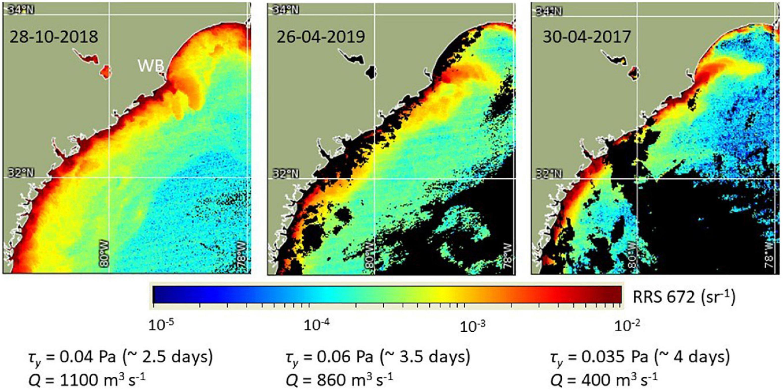
Figure 1. VIIRS images of sediment index Rrs at 672 nm of the South Atlantic Bight shelf and the Winyah Bay (WB) plume. The forcing conditions shown below images are: freshwater discharge Q (Pee Dee only) over the preceding 5-day period, and the magnitude (duration) of the upwelling-favorable wind stress defined as its meridional component τ_y.

Similar cross-shelf plume structures were reported previously in other regions. For instance, Li et al. (2003) presented satellite images of cross-shelf fronts, also in the SAB, but ∼200 km farther south from our study site. In that study the authors acknowledged the role of the wind forcing, but they did not link these features to estuarine outflows nearby. Other examples include the Columbia River plume studies, e.g., [Hickey et al., 1998 (their Figure 5B)], and [Hickey et al., 2009 (their Figure 13, central panel)], as well as the Fraser River plume observations reported by Kastner et al. (2018). In these studies, the observed offshore extension of buoyant water was due to the wind forcing opposing the natural downstream propagation of a plume. However, the continental shelf of the United States west coast is narrow so that the Columbia River plume is exposed to open ocean dynamics as it spreads offshore, while the cross-shore spreading of the Fraser River plume is limited by the width of the Strait of Georgia.

The response of a coastal plume to the upwelling-favorable wind has been extensively studied previously (e.g., Münchow and Garvine, 1993; Xing and Davies, 1999; García Berdeal et al., 2002; Whitney and Garvine, 2005; Lentz and Largier, 2006; Fisher et al., 2018; among others). Several works addressed the response of a far field (e.g., Fong and Geyer, 2001; Lentz, 2004) where the buoyant layer can be approximated by a slab model with horizontally uniform density. The buoyant water is transported offshore by the Ekman dynamics associated with the alongshore wind stress, while the mixing occurs at the offshore edge of a plume where the interface outcrops to the surface and consequently the bulk Richardson number drops below the critical value. Within the bulge area, both the alongshore and high-frequency cross-shore wind components can be important in transporting the buoyant water (e.g., Kakoulaki et al., 2014), while spatially homogeneous density field cannot be assumed due to the presence of a buoyancy source. Previously, Yankovsky and Voulgaris (2019) presented observations of the WB plume under light upwelling-favorable wind conditions and found the existence of interior fronts within the bulge. They hypothesized that interior fronts are formed by successive tidal pulses of the estuarine outflow undergoing rotational adjustment while being exposed to the wind-induced offshore transport. The proposed mechanism is somewhat similar to the formation of interior front discussed by O’Donnell (1990) (referred to as an interior jump herein), albeit under the influence of the alongshore mean flow, not the wind stress. Yankovsky and Voulgaris (2019) also argued that interior fronts are characterized by enhanced mixing due to the superposition of wind-induced and geostrophic shear; however, no mixing data were available for their study.

This study continues the investigation of the WB plume and its salient features under upwelling favorable wind forcing previously observed by Yankovsky and Voulgaris (2019). Measurement techniques are now expanded and yield additional information: near-surface salinity and velocity, as well as vertical profiles of the turbulent kinetic energy (TKE) dissipation ε. The supercriticality of a plume (and its interior front in particular) is assessed by solving a boundary problem for internal waves in the presence of the continuous stratification and sheared mean current. Most previous studies defined a supercritical regime in a highly simplified way, assuming a slab-like buoyant layer of a constant density and making a hydrostatic approximation. When these assumptions are relaxed, internal waves become dispersive, which implies that supercritical conditions can exist only for a limited range of wavenumbers. Moreover, change of the vertical shear with depth in the frontal current acts as a restoring force additional to the buoyancy effect (e.g., Baines, 1995).

The rest of the paper is organized as follows: section “Materials and Methods” describes the data collection and processing; section “Results” presents the results of data analysis; section “Internal Wave Properties” revisits the definition of the supercritical plume and delineates properties of internal waves under the observed conditions; and section “Discussion and Conclusion” discusses and summarizes the results. Derivation of the eigenvalue problem for internal waves in the presence of the mean sheared current and its numerical solution is described in Appendix.

Materials and Methods

The WB plume was sampled on March 11, 2020 from 11:00 through 20:00 (all times are UTC) from the RV Coastal Explorer. A total of 16 stations were completed along a zonal transect running offshore from the WB mouth (Figure 2). The first station was conducted ∼1.1 km due east from the end of the southern (longer) jetty, or 8.1 km from the coast. Spatial separation between the stations was slightly less than 1 nautical mile. As seen from the inset in Figure 2, the transect was aligned with the direction of the plume’s maximum offshore extent. The observations comprised ADCP measurements from the ship, microstructure profiling, CTD casts with the SBE 19plus v2 probe, and surface current measurements from a drone. The RV Coastal Explorer is a catamaran, and the 1200 kHz Workhorse Sentinel ADCP was deployed on a vertical pole between the bows with a bin size of 0.25 m and the center of the first bin referred at 2.58 m below the sea surface. The ship draft is 1.4 m, and hulls did not affect currents in the uppermost bin. ADCP sampling was interrupted from 16:38 through 17:18 (early station 10 through mid-station 11). Microstructure was sampled with two Rockland Scientific profilers: VMP-250 (downward profiles, stations 2–16) and MicroCTD (uprising profiles, stations 2–12). Both instruments had JFE-Advantech temperature and conductivity sensors which yielded temperature T and salinity s profiles in addition to the TKE dissipation rates. Microstructure profilers were deployed from a diver platform at the stern (facing upwind during sampling). Typically, three casts were completed with each instrument, which took on average 10 min. The ship was drifting predominantly downwind (not with the current) and if its position changed by 100 m or more during the sampling, it maneuvered back to the designated station location between the microstructure measurements and the CTD cast. The drone operations followed the CTD cast and were performed at stations 3 through 15.

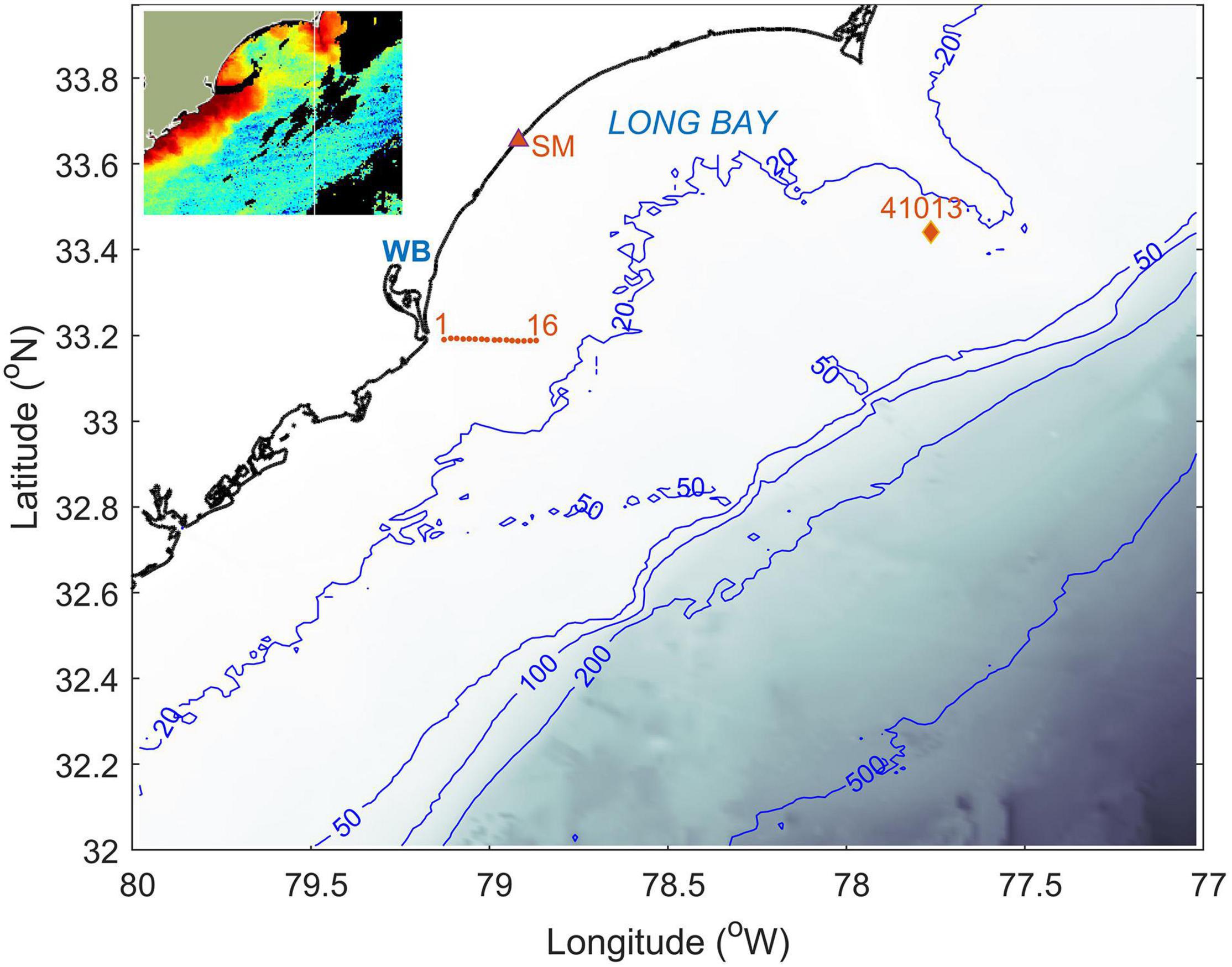
Figure 2. Study area showing the data collection stations 1–16 (asterisks), NOAA NDBC buoy 41013, and the NOAA tide gauge station Springmaid Pier (SM). Isobaths are shown in meters. Inset is the satellite image (the same property and color scale as in Figure 1) corresponding to the map area and obtained on March 11, 2020 at 16:53–18:41. Images adapted from NOAA Coastwatch/Oceanwatch.

Auxiliary data include freshwater discharge measurements from the USGS streamflow station 02135200 Pee Dee River at Highway 701 near Bucksport, SC (∼72 km from the WB mouth), sea level from the NOAA tide gauge station 8661070 at Springmaid Pier (33.655 N, 78.918 W), and offshore atmospheric forcing data from the NOAA buoy NDBC 41013 (33.441 N, 77.764 W) (Figure 2). Wind speed observations were available from the meteorological tower at the WB mouth (utilized in Yankovsky and Voulgaris, 2019) but no wind direction due to wildlife nesting. Comparison of wind velocity magnitude from the NOAA buoy and the tower show good agreement during the second half of March 10 through the first half of March 11 (wind forcing which affected the observed plume), while wind remained light during the mid-day of March 11 (Figure 3). Synthetic aperture radar (SAR) satellite image of the plume captured on March 12, when the forcing conditions remained similar to the period of shipboard observations, was obtained from the European Space Agency.

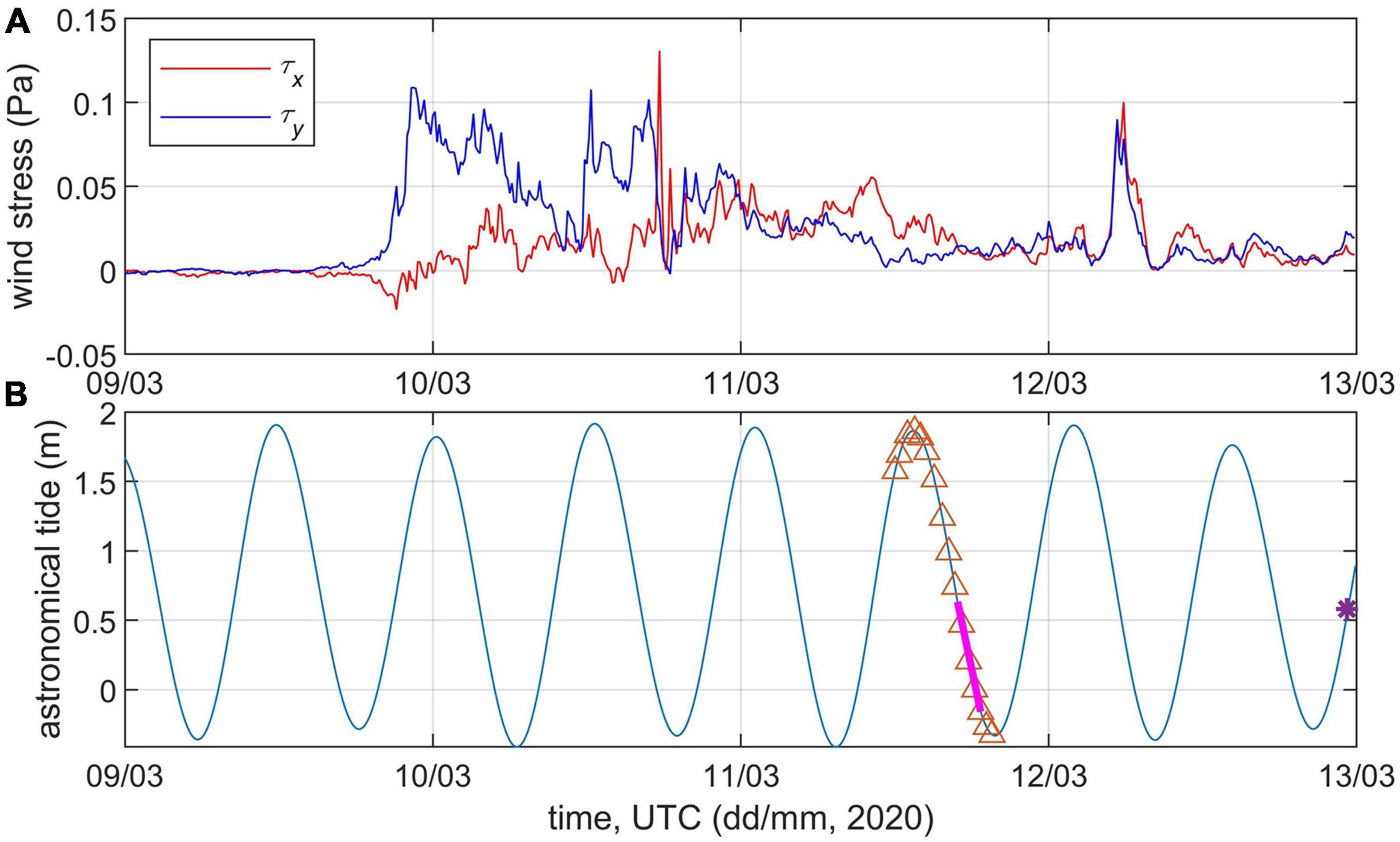
Figure 3. Time series of (A) zonal (x) and meridional (y) components of the wind stress derived from the NDBC 41013 buoy data; (B) tidal sea level oscillations at Springmaid Pier station. Triangles, heavy magenta line and asterisk represent times for oceanographic stations, data collection for inset image in Figure 2, and SAR image, respectively.

A straight line was fit to nominal locations of the stations (corresponding to CTD casts) and the projection of the measurement location on this line is referred to as the transect distance, with zero corresponding to the first station and the positive direction pointing eastward. A Cartesian coordinate system with x-, y-, and z-component pointing eastward, northward, and upward, respectively, is applied to vector quantities.

ADCP data were averaged over 5-min time intervals immediately preceding the drone sampling (and thus overlapping CTD casts). These ADCP profiles were combined with spatially averaged near-surface currents derived from the drone (see below). As an additional quality control, we estimated spatially averaged coordinates of the drone-derived surface currents (from drone GPS), and temporally averaged coordinates of the ADCP-derived currents (from the ship GPS). In almost all cases, their discrepancy was less than 100 m, typically ∼50 m or less, and in two cases as low as ∼ 10 m. The only exception is the separation of 240 m at station 10 due to the gap in ADCP record (so that earlier in time ADCP data were averaged, taken during the microstructure sampling).

The data from the two microstructure profilers were processed in similar ways to obtain estimates of ε. For efficiency, we will refer to the VMP-250 as dc (downcast) and the MicroCTD as uc (upcast). Dissipation estimates were obtained using Rockland Scientific processing tools (Lueck, 2016). Default cutoffs for spectral integration using the Nasmyth spectra vs. fitting to the inertial subrange were used. Each spectrum was the average of individual spectra obtained from 2-s segments with 50 and 75% overlap for the dc and uc systems, respectively. In order to maximize vertical resolution, in particular near the surface, a 4 s record was used for estimating the spectra. The minimum depth for evaluation was 1 m (dc) and 0 m (uc). Additionally, a minimum vertical velocity was set at 0.4 ms^–1 (dc) and 0.45 ms^–1 (uc). Terminal speeds were approximately 0.5 ms^–1 (dc) and 0.6 ms^–1 (uc). Dissipation estimates at the start of the uc cast (near bed) were manually removed if they did not agree with the dc estimates, or if there was high vibration, likely resulting from the instrument moving through its own wake after releasing its weight. Vertical tilt did not exceed 10° for either instrument. Each profiler was mounted with two perpendicular shear probes, and the two measurements were averaged for all analyses shown here. For salinity profiles obtained with JFE Advantech (JAC) sensors on MicroCTD, temperature and conductivity measurements were synchronized using the actual uprising velocity and following the procedure recommended by the manufacturer. The CTD sampling frequency was 4 Hz and the resulting profiles were averaged over 1-s time intervals.

Drone operations consisted of flying a DJI Phantom 4 Pro quadcopter with a 4k rectilinear video camera at the nominal altitude of 120 m (which slightly varied between the stations) and recording 30 seconds of video of the ocean surface with the camera pointed nadir. Video imagery was analyzed in order to identify the surface gravity wave parameters (wavelength, direction, and phase speed). Surface ocean currents produce a Doppler shift in the dispersion relation (change in phase speed) of linear surface gravity waves. The change in phase speed for a particular wave corresponds to the currents at a depth of approximately the wavelength divided by 4π (Stewart and Joy, 1974). The near-surface ocean current velocity was estimated by fitting the linear dispersion relation using the wavelength and phase speed values identified in the video imagery (Horstmann et al., 2017). We limit the wavelengths used in the analysis from 1 to 5 m, thereby providing an estimate of the ocean current at a depth between 0.08 and 0.40 m, with the average depth close to 0.18 m (but varying between stations). This methodology has shown to agree well (RMS differences below 0.1 m/s) with surface current estimates from a boat mounted ADCP (Streßer et al., 2017). The software used for this analysis was obtained from https://github.com/RubenCarrascoAlvarez/CopterCurrents.

The Sentinel-1 level 1 GRD product was processed using the European Space Agency’s Sentinel Application Platform (SNAP¹), following the generic workflow process described in Filipponi (2019). The steps included were (1) updating of the orbit state vectors for the image by applying the precise orbit available in SNAP; (2) thermal noise removal; (3) removal of low intensity noise and invalid data on the edges of the image (border noise removal); (4) conversion of the digital pixel values to radiometrically calibrated SAR backscatter using the calibration equation included within the Sentinel-1 GRD product; (5) removal of granular noise through Speckle filtering; (6) range Doppler terrain correction to obtain a precise geolocation information; and (7) conversion of backscatter to dB.

Results

The observed plume was formed under conditions of high discharge, moderate-to-light southwesterly wind (meteorological convention) and spring tides (Figure 3). In general, the upwelling conditions are associated with the alongshore wind stress component pointing upstream (i.e., northward), which causes a divergence in the corresponding cross-shore Ekman transport at the coast. The coastline orientation changes abruptly at the WB mouth (Figure 2). Since subinertial signals propagate along the shelf in the downstream (i.e., southward) direction only as coastally trapped waves (e.g., Yankovsky and Garvine, 1998) we assume that the upstream, meridionally oriented segment of the coastline adjacent to the WB mouth plays a more important role in controlling the upwelling conditions. Hence, we consider the northward component of the wind stress as upwelling-favorable. The upwelling-favorable wind event started at the end of March 9 and continued uninterrupted for ∼1.5 days by the beginning of data collection (Figure 3A). The alongshore wind stress was stronger (up to 0.1 Pa) on March 10 and subsided to less than 0.05 Pa on March 11, when the observations started. In addition, there were high frequency gusts in the eastward direction, which could also contribute to the offshore transport of the buoyant water. The tidally averaged Pee Dee River discharge prior to the observations was gradually decreasing from over 1000 m³ s^–1 in early March and attained near-constant values of 765–775 m³ s^–1 from the second half of March 8 through the period of observations. Both the discharge (assuming some delay between the discharge measurements and freshwater arrival on the shelf) and tidal amplitude were higher than those reported by Yankovsky and Voulgaris (2019). Overall, conditions were favorable for the formation of a cross-shelf plume although the duration of the upwelling favorable wind was shorter than in the cases from Figure 1. Hence, we assume that our observations represent an early stage of the cross-shelf plume formation, when its distinctive elongated shape has not yet been fully developed. This assumption is supported by the satellite image inset in Figure 2, showing a tendency for the offshore spreading of the WB plume. We also note that according to the scaling from Yankovsky and Voulgaris (2019) (their Figure 11), the observed conditions support the formation of interior fronts separating relatively older and younger tidally discharged water within the plume.

Before proceeding with presenting the in situ measurements, it is instructive to examine the spatial structure of the newly formed tidal plume observed on March 12 (Figure 4). The SAR image was obtained 2 h past the low tide (Figure 3B), thus the tidal pulse from the previous ebbing cycle was fully released, and the wind forcing at this time was very light, ∼0.02 Pa (Figure 3A). The width (i.e., its zonal dimension) of this tidal plume is 10–11 km, and the plume is clearly separated from the coast, which is likely due to the presence of jetties. Due to the similarity of forcing conditions, we assume that tidal pulses like this were present during the data collection period on March 11. Also, the tidal plume is shifted upstream (to the north) from the mouth, which further justifies the choice of the northward wind stress component as a proxy for the upwelling-favorable forcing.

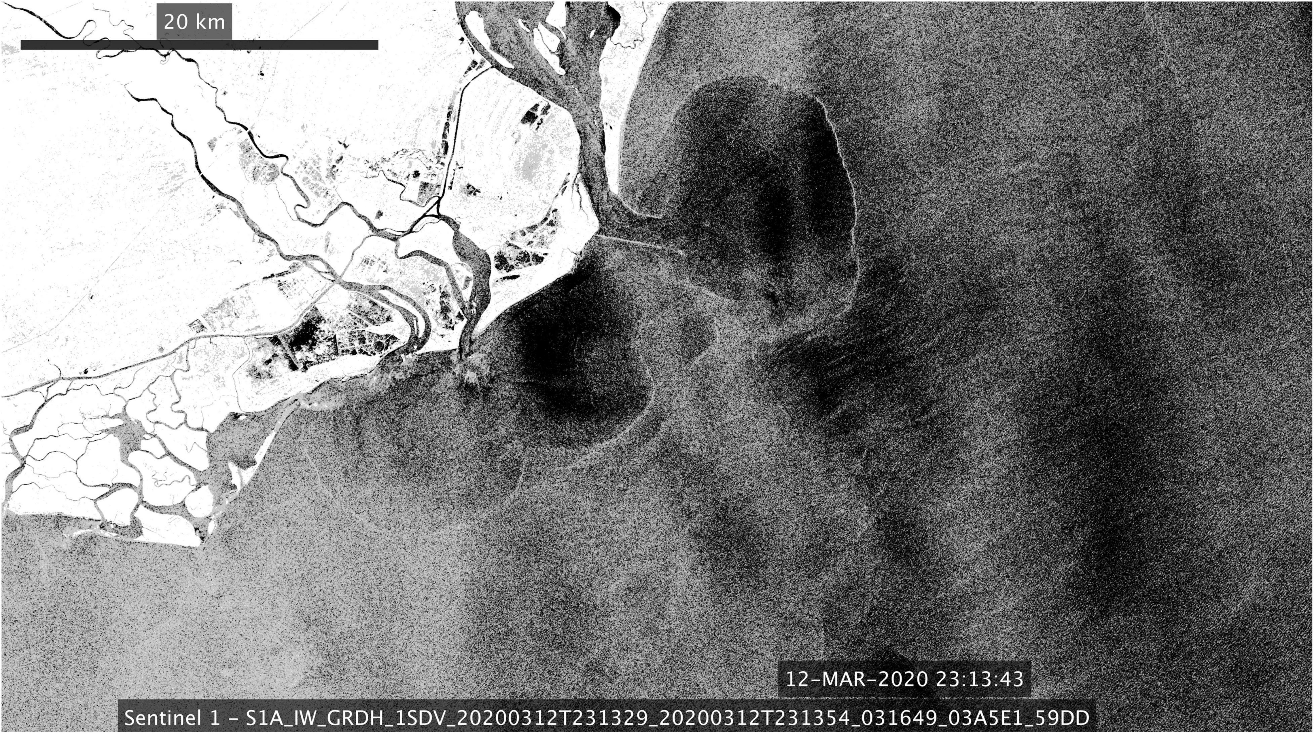
Figure 4. Synthetic aperture radar image of the tidal plume off Winyah Bay obtained on March 12, 2020 at 23:14.

The hydrographic structure of the water column was sampled with both the conventional lowered CTD probe and with two microstructure profilers; Figure 5 compares the resulting salinity profiles. Only stations 2 through 12 are shown, where the MicroCTD data are available. There is a tendency in CTD measurements to indicate a deeper halocline compared to MicroCTD profiles, especially at the nearshore stations 2 through 6, where the plume was shallower. This discrepancy is attributed to the ship’s internal wake caused by its wind-induced drift (relative to the surface current). The MicroCTD profiler was deployed on a loose tether and surfaced at 5–10 m away from the ship, hence its data were less contaminated by ship’s wake. Another advantage of the MicroCTD is that it sampled the near-surface layer up to 10–15 cm from the surface. VMP-250 salinity data are not discussed here because they do not offer any advantage over CTD due to its dc mode of sampling. The plume remained shallow, ∼4 m or less, with the 1–1.5 m deep, low salinity (minimum s ∼18–20) layer on top. Some profiles exhibit step-like structures (e.g., stations 3, 5, 10, 11) associated with more mixed, previously discharged buoyant water (recall a stronger wind forcing on the previous day, see Figure 3A).

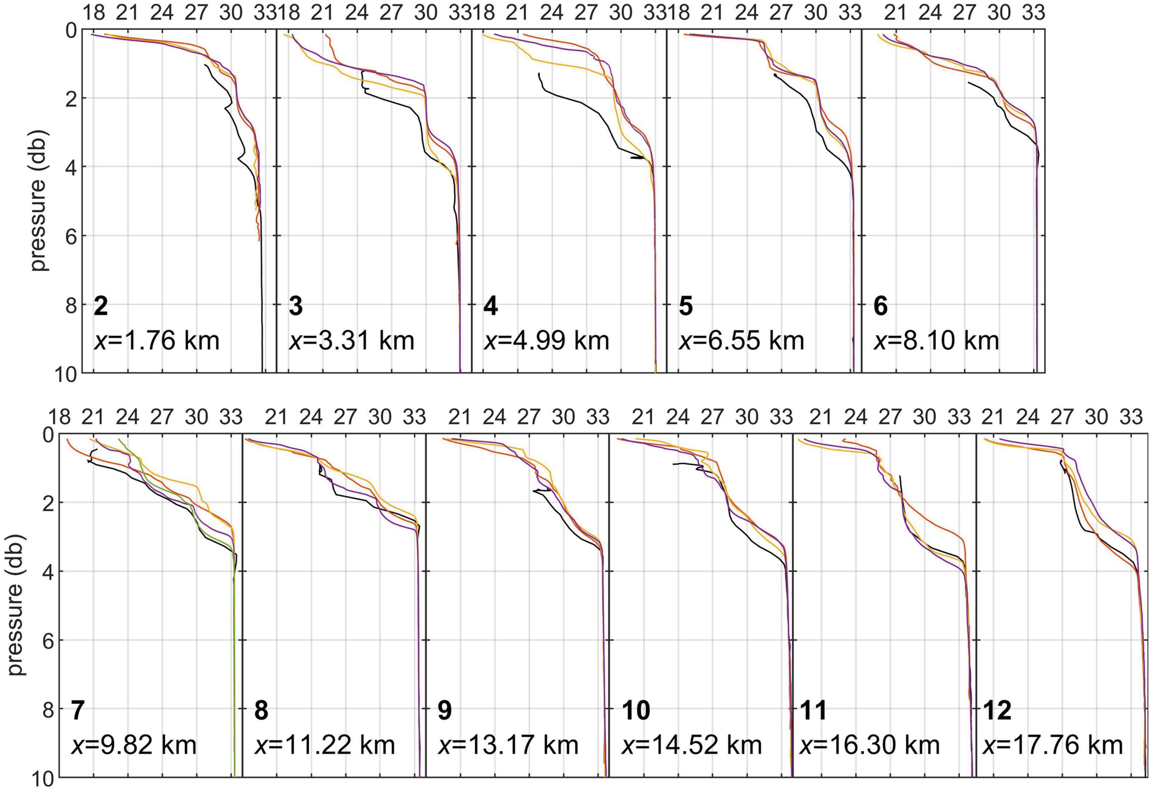
Figure 5. Salinity profiles at stations 2–12: black – CTD casts, in colors – multiple MicroCTD casts. Salinity scale is the same in all panels. Station number and the corresponding transect distance are shown at the bottom of each panel.

Despite the potential influence of the ship’s wake, CTD measurements are suitable for TS analysis (Figure 6) and reveal that the plume extended offshore past station 16 (with a corresponding transect distance of 24.06 km). This implies that the plume spread more than 30 km eastward from the coast, consistent with the satellite image inset in Figure 2. Water column stratification was primarily due to salinity, with temperature contribution being small. However, temperature is a good indicator for the age of the buoyant water, since the newly discharged water was cooler than the ambient shelf water. This is illustrated in the TS diagram of all 16 CTD stations shown in Figure 6, where data can be separated into three clusters according to the temperature range of the low-salinity buoyant layer. Stations 1–9 with the lowest T represent the newly discharged water, stations 10–14 represent intermediate age of the plume, and outer station 15–16 have the warmest and oldest water. Transition between these clusters is not abrupt: for instance, the lower part of the plume at station 9 has characteristics closer to the intermediate part of the plume (station 10), while the TS curve of station 15 also merges at some points with intermediate stations 14 and 12. However, stations 10–14 have almost identical TS indices of ∼14.8°C and ∼29, respectively (shown with red circle in Figure 6) indicating homogeneous water properties at some mid-depth layer of the plume. We deduce that this “mode water” in the intermediate part of the plume undergoes slower transformation than in the layers above or below.

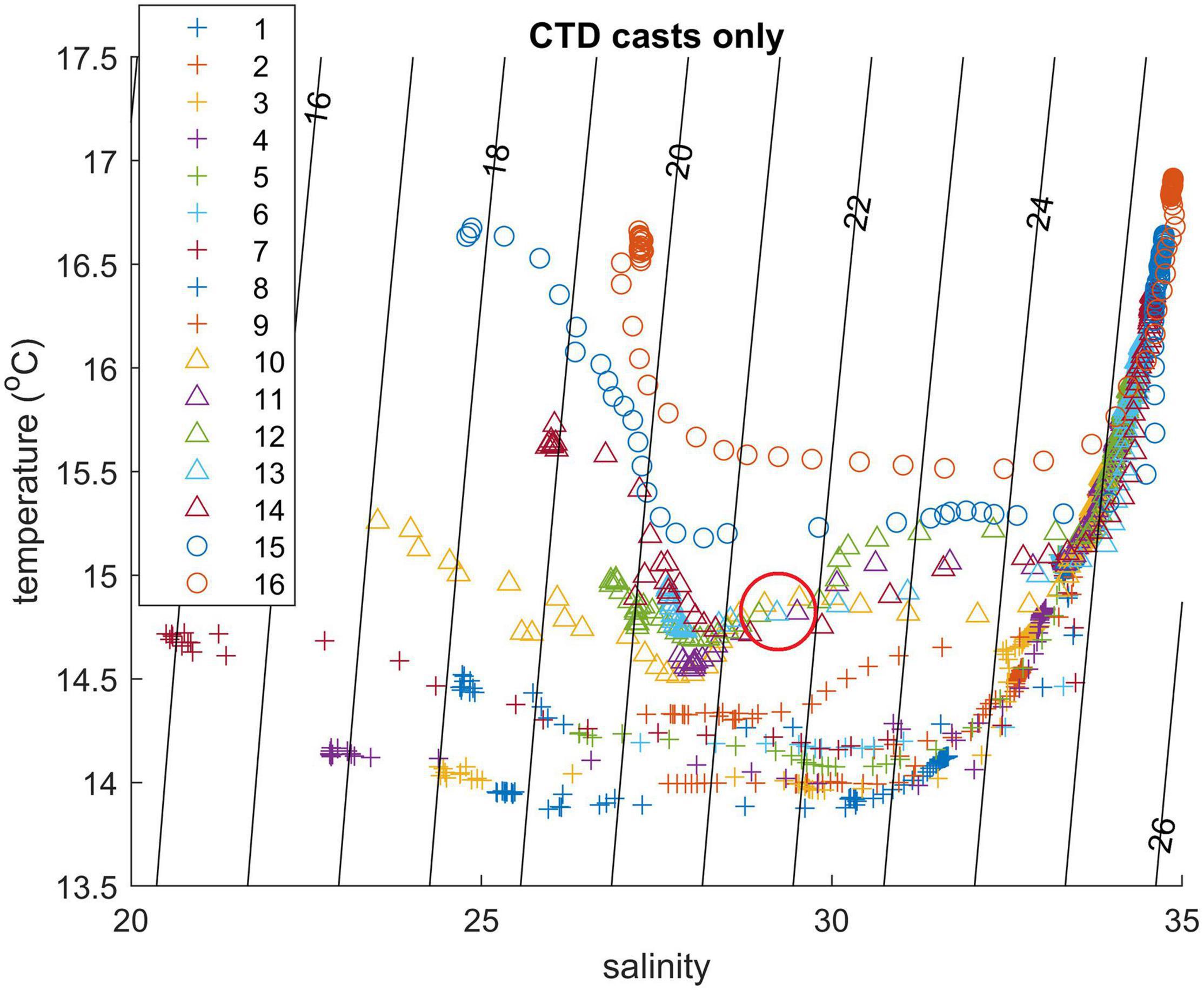
Figure 6. TS diagram from CTD casts. Station numbers are shown in the legend; red circle emphasizes uniform TS properties of the buoyant layer between several stations.

The drone-derived surface currents exhibited a highly spatially variable, eddying flow regime near the mouth (stations 3–5, see examples in Figures 7A,B) with a predominantly offshore direction. The average radius of curvature r in surface currents at station 3 was ∼70 m and was determined from 8 pairs of vectors as r = d/tan⁡(△φ), where d is the distance between the two vector locations along the stream line, and Δφ is the difference between their direction. Vortical structures seen at stations 3 and 4 cannot be directly caused by the energetic estuarine outflow because these samples were taken during the flood (Figure 3B). We believe they are associated with submesoscale processes on the inshore plume front under the upwelling wind forcing. From stations 6 through 15, the near surface flow was predominantly southeastward, consistent with the direction of the Ekman drift associated with the observed southwesterly winds (e.g., Figure 7C). Some directional variations in surface currents did occur between the stations, since the wind stress-induced flow was not the only component present at the surface.

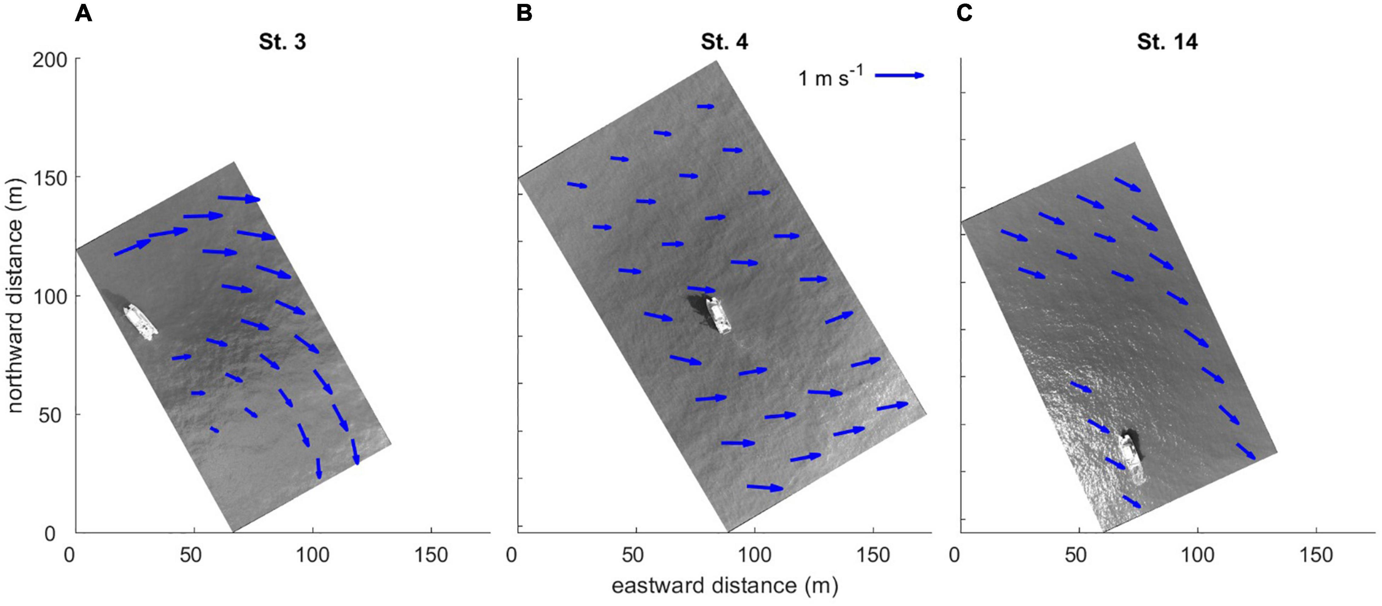
Figure 7. Examples of drone-derived near-surface velocity field at (A) station 3; (B) station 4; (C) station 14.

Combined drone-ADCP current profiles for all stations where drone data are available are presented in Figure 8. Drone-derived velocities are referred at near-surface depth varying from 0.13 to 0.22 m between different stations depending on spectral characteristics of the surface wave field. Near surface (drone-derived) currents have an offshore (eastward) component associated with the upwelling favorable wind. Since the prevailing wind was from southwest, the Ekman drift should have a southward component. Currents at 2.5–4 m depth show the anticyclonic flow pattern associated with the plume: the upstream flow at inshore stations 3–5 and the downstream flow at offshore stations 11–15. Strong vertical current shear is present in the upper part of the water column, apparently associated with the buoyant plume and the action of wind stress. The lower portion of the water column is dominated by tidal currents, which is evident in the vector rotation between the stations which follows the tidal stage: tidal currents turn seaward–southward–shoreward as tidal stage progresses from high tide to low tide (compare Figure 8 and Figure 3B where timing of measurements is shown against the tidal stage). There is a velocity minimum in the lower part of the buoyant layer seen in the offshore stations 9–15. While this minimum is not fully resolved due to the vertical gap between the drone- and ADCP-derived currents, this feature is consistent with the presence of a homogeneous “mode” water at the mid-depth of the plume (stations 10–14).

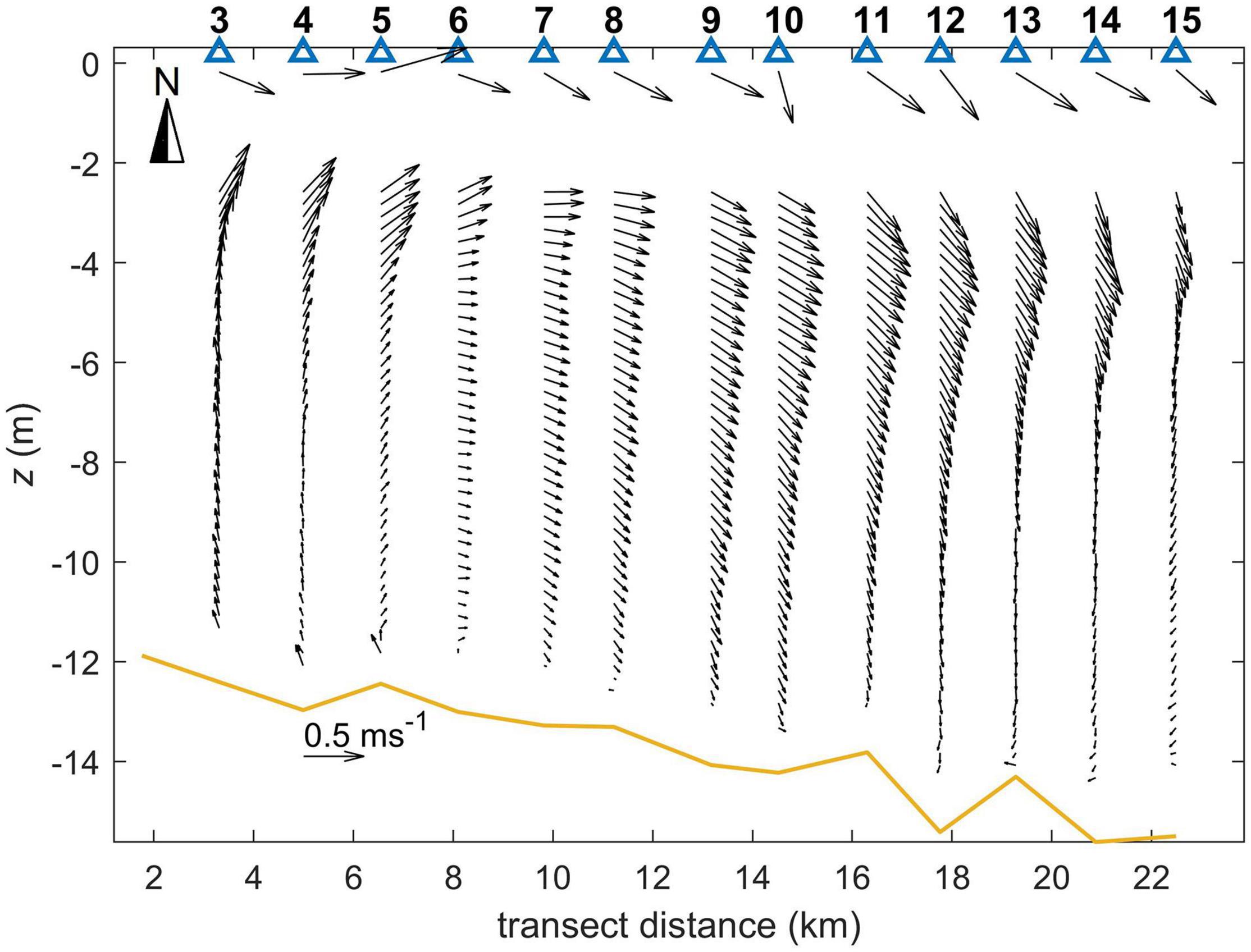
Figure 8. Combined drone-ADCP vertical profiles of horizontal velocity vectors, stations 3–15. Heavy line is the bottom.

The vertical distribution of salinity along the transect (Figure 9A) is constructed from MicroCTD casts. As explained earlier, these data are not contaminated by the ship’s hull interference and also resolve the near-surface structure of the plume. For each station (2 through 12), individual casts were projected into 0.1 m vertical bins and averaged. Figure 9 shows a newly formed tidal plume that occupies transect distances of ∼2–12 km as a thin (less than 2 m) buoyant layer with the lowest near-surface salinity below 20. Its cross-shelf length scale is comparable with that shown in the SAR image (Figure 4). The tidal plume is detached from the coast and forms an inshore front at ∼2 km. There is a convergence of buoyant water near the front, at 2–4 km. The vortical feature seen in surface currents (Figure 7A) at station 3 (x = 3.3 km) corresponds to this frontal convergence zone. The older, previously discharged buoyant water lies below and offshore of the new tidal plume, where another convergence zone exists at x = 12–14 km (stations 11–12). This feature appears to be an interior front similar to described in Yankovsky and Voulgaris (2019). At stations 11–12, the strongest stratification occurs at the base of the buoyant layer, while isohalines 28 and 30 (yellow–orange colors) have the widest separation. According to Figure 6, this is a layer occupied by the homogeneous “mode” water, and its depth of ∼1.9–2.5 m corresponds to the velocity minimum (Figure 8).

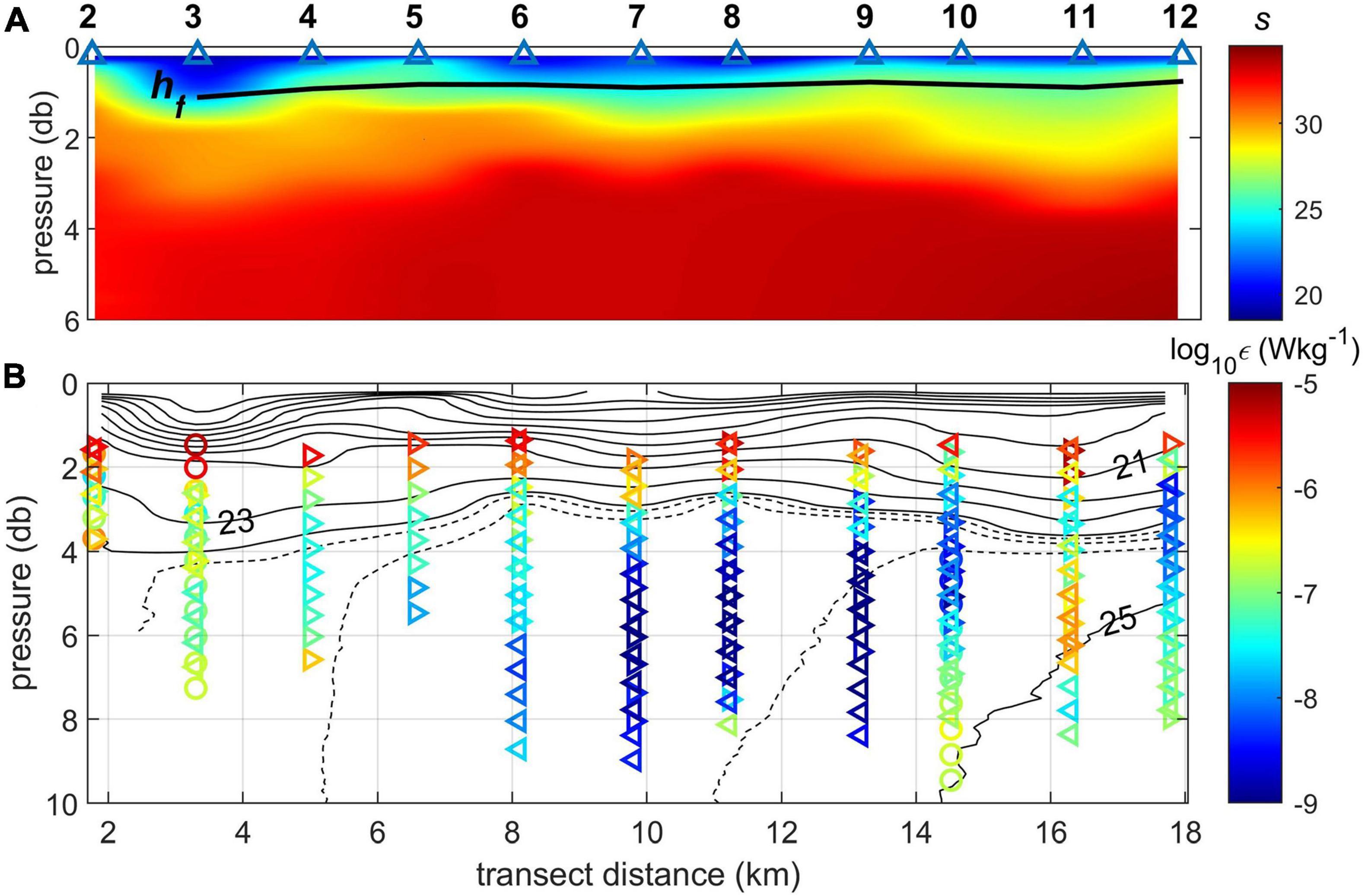
Figure 9. Vertical transects derived from MicroCTD measurements, stations 2–12: (A) salinity with corresponding freshwater layer h_f; station locations are shown at the top; (B) TKE dissipation (color, different symbols represent different casts) and density σ_T (black contours). Contour intervals are 1 kg m^–3 (solid line) and 0.25 kg m^–3 (dashed line).

The spreading of the plume can be characterized by its freshwater content h_f which was estimated as

where z_r = −8 m and s_r = 34.9 is the reference salinity (the highest salinity on the transect observed at station 16). The freshwater content was determined using the upper 8 m of the water column, roughly twice the depth of the plume. Higher values of h_f inshore (x ≤ 6.5 km) are mostly due to lower salinity at depths 4–8 m, which does not necessarily represent the spreading of newly discharged water during the ongoing upwelling event. Farther offshore, h_f remains fairly uniform: the average of stations 5–12 is 0.84 m, with the maximum of 0.90 m found at station 11 (x = 16.3 km) and the minimum of 0.76 at station 12 (x = 17.8 km).

Next, we discuss the TKE dissipation rates. In general, VMP and MicroCTD profiles showed a good agreement. While the ε magnitude at specific depths varied between consecutive profiles due to high intermittency of turbulence in a highly stratified coastal environment (e.g., Huguenard et al., 2019), the shape of profiles remained remarkably consistent for each station. Since uprising profiles of MicroCTD provided better near-surface resolution (within the plume), only those are shown in Figure 9B. Although three MicroCTD profiles were conducted at each station (four at station 7), some of them were discarded due to the applied screening criteria. For this reason, we do not average individual profiles of ε for each station (as it was done for salinity) but show all of them with different symbols (Figure 9B). In the newly discharged buoyant water, high ε values of O(10^–5–10^–6)W kg^–1 penetrate to the base of the buoyant layer (especially at x = 8–11 km, Figure 9B), while below the plume ε drops to values lower by several orders of magnitude. In the intermediate age plume, ε decreases to ∼10^–7 W kg^–1 in the lower part of the plume where stronger stratification is present. Interestingly, there is a local maximum of ε below the base of the plume (∼5–7 m depth) at the location of the interior front (x = 16.3 km). This local maximum is also seen in two of three VMP profiles at station 11 (not shown), although the depth of the maximum, as well as its magnitude change between the individual profiles. This mid-depth maximum appears to be a robust feature and can be caused by the internal wave dynamics. It is well documented that energetic tidal pulses of buoyant discharge generate internal waves which radiate into an existing plume (e.g., Nash and Moum, 2005; Jay et al., 2009). Alternatively, ε mid-depth maximum can be present due to bottom friction of tidal currents, as reported by Spicer et al. (2021). However, no similar local maxima were observed inshore (6 < x < 14 km), where the water depth is approximately the same.

Vertical profiles of the horizontal velocity vector were projected on the direction of the integral depth-averaged velocity in the top 6 m layer (representative of the buoyant layer) for each station, and are referred to as maximum velocity profiles. They are shown in Figure 10A for offshore stations (starting from 8), where the subsurface velocity minimum occurred. While this velocity minimum is not fully resolved due to the vertical gap between the drone- and ADCP-derived currents, it is consistent with the presence of a homogeneous “mode” water at the mid-depth of the plume (stations 10–14). Its likely cause is the superposition of wind-induced shear stresses and the baroclinic pressure gradient. The former operates in the upper part of the plume which is evident in the vertical distribution of ε (Figure 9B) and causes the veering of the velocity vector with depth (Figure 8).

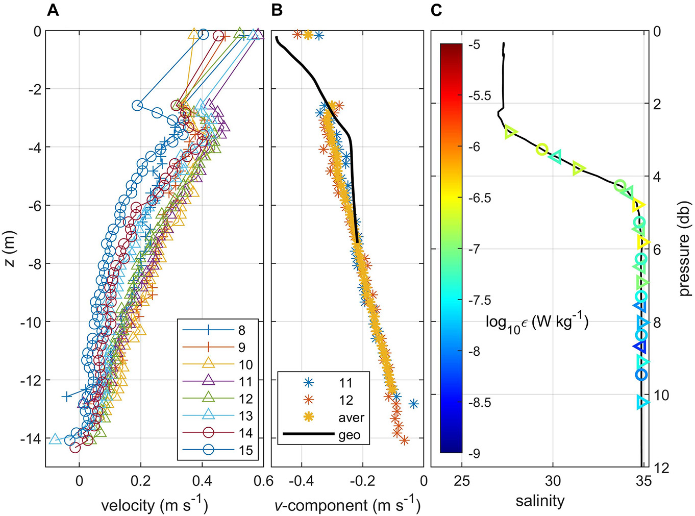
Figure 10. Vertical profiles of (A) maximum velocity, stations 8–15; (B) meridional velocity component at the interior front, stations 11–12, their averaged value and geostrophic estimate; (C) salinity and TKE dissipation at station 16, different symbols indicate different casts. For comparison, the same color scale is used as in Figure 9.

We deduce that in the older, offshore part of the plume (x > 12 km) the Ekman flow occupied only the upper part of the buoyant layer, which is evident in the decrease of ε, velocity minimum, and a more homogeneous “mode” water all occurring below 2 m, while the actual depth of the plume was ∼ 4 m. To further support this conclusion, we estimate the Ekman depth h_E as described below. We assume that the plume is linearly stratified with the constant buoyancy frequency N defined as

where g is the acceleration due to gravity, where Δ_ρ0 = 25.84 kg m⁻³ is the density anomaly of freshwater relative to the salinity at the base of the plume (assumed to be ∼34), ρ is the reference density and h_p is the depth of the plume. Next, we assume that the Ekman velocity changes linearly with depth and vanishes at the base of the Ekman layer h_E. With this assumption, the vertical shear $u_E^{{}^{\prime }}$ is defined

where τ is the wind stress and f is the Coriolis parameter. Finally, we assume that the Ekman layer reaches the depth where the gradient Richardson number comes to its critical value of 0.25:

Using the following observed values: τ = 0.03 Pa, h_p = 4 m, h_f = 0.84 m, f = 8 × 10^–5 s^–1, and ρ = 1020 kg m^–3 yields h_E = 1.8 m, which is in a very good agreement with the observed structure of the plume.

Station 11 has been identified as the location of the interior front: it is characterized by the buoyant water convergence and the deepening of isopycnals. This station also has the fastest velocity of the buoyant layer as seen in the maximum velocity profiles (Figure 10A). We estimated geostrophic velocity between stations 11–12 using the observed v-component at mid-depth as a reference and integrating the geostrophic shear upward (Figure 10B). The geostrophic velocity in Figure 10B is compared against the observed v-component (average of velocity profiles from the two stations). Clearly, there is significant geostrophic component in the observed velocity field at stations 11–12, although turbulent stresses tend to “smooth” the velocity profile and make it more linear with depth, as was also reported by Yankovsky (2006) and Mazzini et al. (2019).

Now we discuss the most seaward station 16 which lacks near-surface information as no drone or MicroCTD sampling took place. The CTD data reveal that the buoyant layer was well mixed (Figure 10C), thus it is permissible to calculate h_f by extrapolating s at constant value to the surface. This yields an h_f value of 0.80 m, which is close to the average of stations 5–12. TKE dissipation rates from the VMP-250 profiler reveal the mid-depth maximum at the base of the pycnocline in two of the three conducted profiles similar to that seen in Figure 9B (x = 16.3 km, station 11).

The observed values of h_f = 0.8–0.9 m, and the reduced gravity g′ = 0.25 ms^–2 associated with the freshwater relative to the ambient water of s = 34.9 density difference yield the internal wave phase speed $C=\sqrt{(g^{{}^{\prime }}{h}_f)}=0.45-0.47$ ms⁻¹. This phase speed is less than the surface velocities from the maximum velocity profiles shown in Figure 10A, which implies that the plume remains supercritical. However, this is a crude estimate based on the slab-like approximation, and this conclusion is further investigated in the next section by considering internal wave properties.

Internal Wave Properties

In this section we consider characteristics of internal wave modes under the observed conditions, in the presence of the vertically sheared mean current. In particular, we focus on the interior front at station 11 where the accumulation of buoyant water occurred and the maximum velocity profile attained higher speed than at any other station. We numerically solve the wave problem Equations A7, A8 derived in Appendix, with H = 14 m, a spatial resolution Δz = 0.05 m, and the horizontal coordinate aligned with the direction of the maximum velocity. In order to elucidate the effect of mean sheared current, we start with somewhat idealized configuration of flow conditions as shown in the inset in Figure 11A: here, the water column is strongly stratified in the upper 4-m layer (N² = 2.4 × 10^–2 s^–2) representing a plume, with weakly stratified lower part (N² = 4.8 × 10^–4 s^–2). The mean current linearly increases toward the surface from 0.1 to 0.3 m s^–1, which is a smaller velocity range than observed. Without a mean current, two wave solutions are possible, forward- (i.e., θ = kx − ωt) and backward-propagating (i.e., θ = kx + ωt) with respect to the x-direction, where θ is the wave phase and the remaining variables are defined in Appendix. When a constant mean current U₀ is added, the dispersion relation ω = ω(k) is modified as:

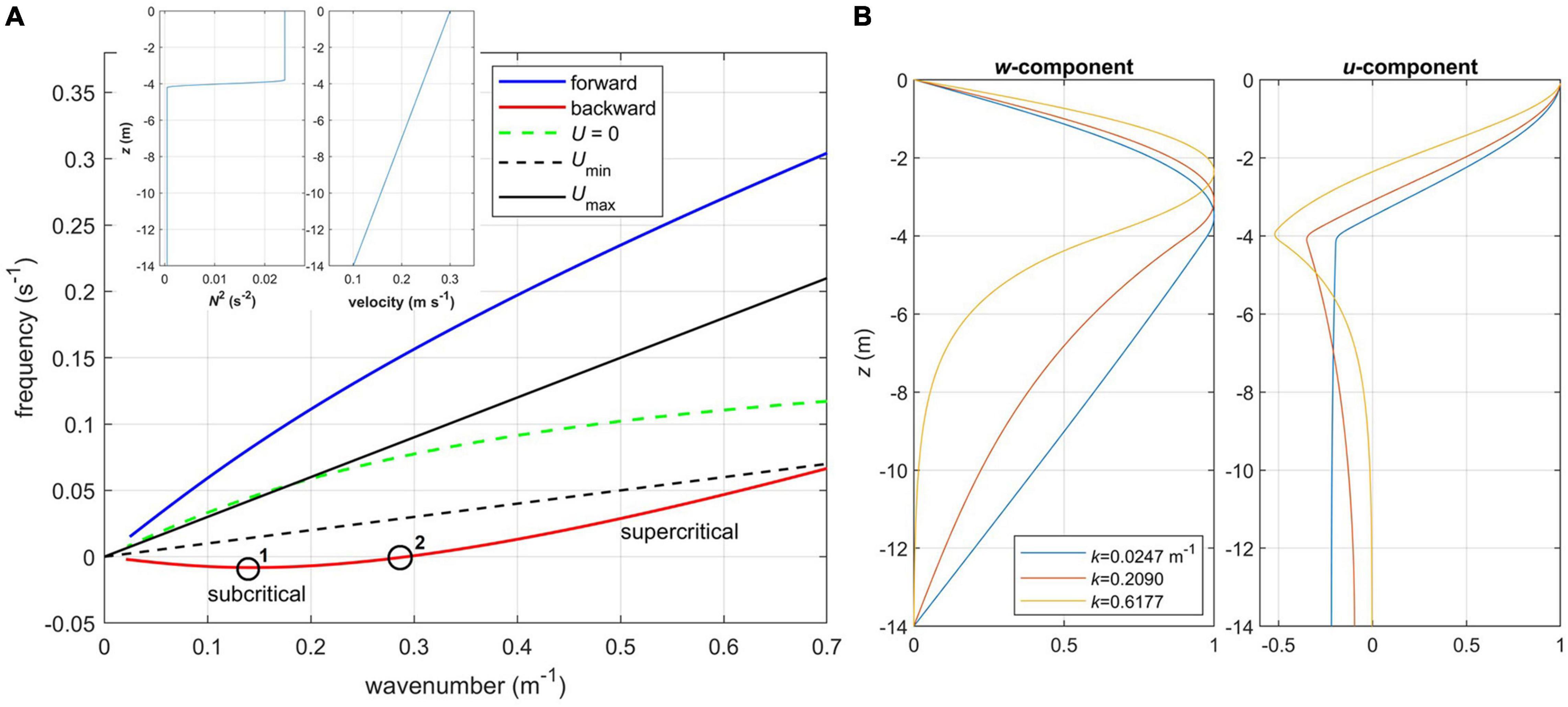
Figure 11. Internal wave properties, case 1: (A) dispersion diagram for the first mode. Points 1 and 2 on the dispersion curve for backward propagating mode are C_g = 0 and C = 0, respectively. Inset shows profiles of buoyancy frequency squared (left) and mean velocity (right) specified in the wave Equation A7; (B) vertical profiles of vertical and horizontal velocity components normalized by their maximum values for various wavenumbers k, forward propagating mode.

where asterisk denotes a Doppler-shifted wave frequency. However, when the mean current changes with depth, the Doppler shift is difficult to deduce without solving a wave problem, because the effective mean velocity depends on the interaction of the mean current with the wave structure (or, alternatively, with stratification). It also should be noted that propagating modes with real ω and k cannot exist with C within the range of mean current velocities, that is, U_min ≤ C ≤ U_max, due to the presence of critical layers.

The resulting dispersion diagram for the first case is shown in Figure 11A; we consider only the first, gravest mode. The forward propagating mode without a mean current is shown as a green dashed line, while the not shown backward propagating mode is symmetric relative to ω = 0. The waves are dispersive, that is, their phase speed C = ω/k decreases with the wave number. Once U(z) is added, backward propagating mode shifts into a positive frequency domain for k ≥ 0.29 m^–1, and remains in a negative frequency domain for lower k. In other words, the mean flow becomes supercritical for shorter waves, and remains subcritical for longer waves. The two points of special interest are those where C = 0 (no wave phase propagation, point 2 in Figure 11A) and where the group velocity C_g = ∂⁡ω/∂⁡k becomes zero (no energy propagation, point 1 in Figure 11A).

It is also instructive to consider the vertical structure of the internal wave velocity field (Figure 11B). Due to the surface-intensified stratification, the wave structure concentrates in the upper layer: horizontal velocity u reaches maximum at the surface, and the u nodal point (where w reaches its maximum) is within the strongly stratified layer, gradually shifting upward with the increasing wavenumber (and frequency). Horizontal velocity of low-wavenumber waves does not change with depth in the weakly stratified layer (z < −4 m), but for waves with higher wavenumbers its magnitude decreases with depth after reaching a local maximum at z = −4m. This is because the wave frequency for such waves becomes higher than N in the lower layer, and the wave behavior there becomes evanescent, exponentially decaying with depth. Only forward-propagating modes are shown, but waves from the lower branch of dispersion diagram exhibit the same tendencies.

In the next example (Figure 12) the maximum U is increased to 0.5 m s^–1, which is closer to the observed values. The backward propagating mode is shifted into the positive frequency domain, that is, the mean current is supercritical for all wavelengths. Also, this mode has a high-wavenumber cutoff, where the dispersion curve merges with U_min. In the backward propagating mode, u-component increases toward the bottom (Figure 12B), and this effect becomes significant as k approaches its cutoff value, that is, C comes close to U_min.

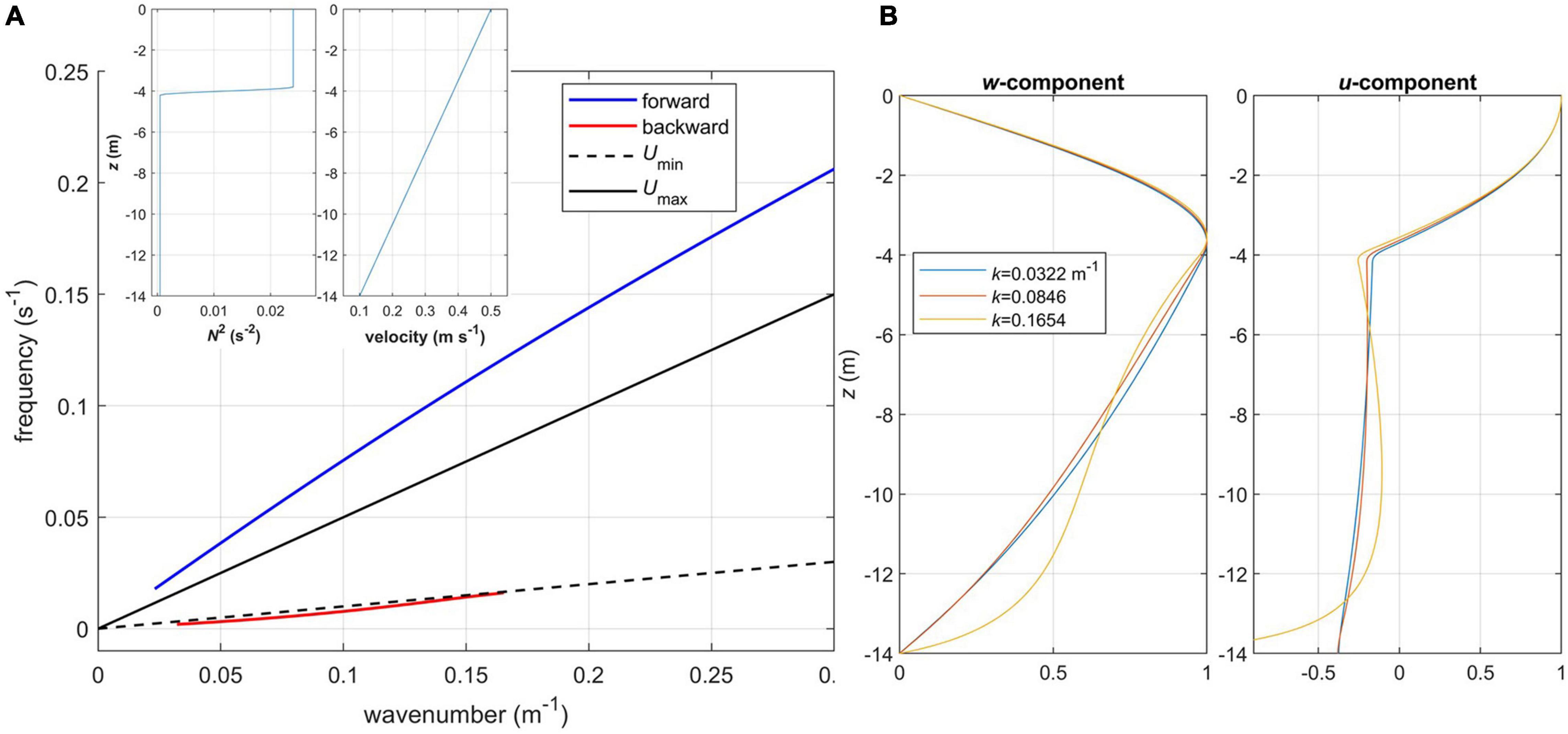
Figure 12. Internal wave properties, case 2: (A) dispersion diagram for the first mode. Inset shows profiles of buoyancy frequency squared (left) and mean velocity (right) specified in the wave Equation A7; (B) vertical profiles of vertical and horizontal velocity components normalized by their maximum values for various wavenumbers k, backward propagating mode.

Finally, the dispersion diagram (Figure 13A) is calculated for the observed profiles of stratification and maximum velocity from station 11. To better constrain a near-surface velocity, the second velocity value was derived from the drone data, for the longer wavelength band and the deeper corresponding reference depth. The mean current profile is approximated with an analytical function (a combination of polynomial and trigonometric functions), which yields its smooth second derivative in the wave Equation A7. Note that since U(z) is now a non-linear function, d²U/dz² acts as a restoring force for wave motions (in addition to the previously discussed Doppler shift). In this case, not only does the mean current become supercritical, but the backward propagating mode is completely eliminated (Figure 13A), while forward propagating waves have even stronger near-surface horizontal velocity maximum and shallower nodal point compared to the previous cases (Figure 13B).

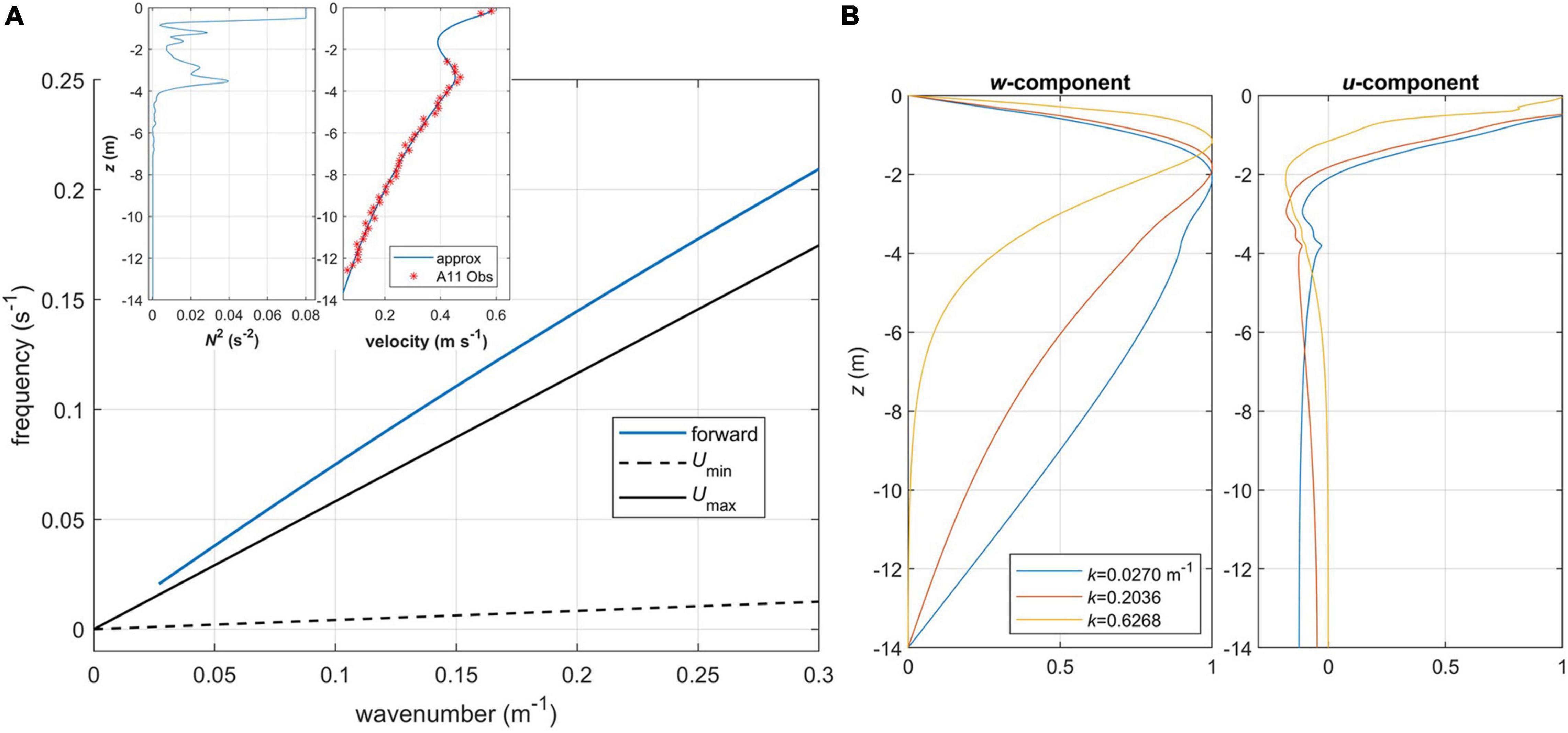
Figure 13. Internal wave properties for realistic conditions from station 11, case 3: (A) dispersion diagram for the first mode. Inset shows specified in Equation A7 profiles of buoyancy frequency squared (left) and mean velocity (right), where asterisks/line show the observed/approximated values, respectively; (B) vertical profiles of vertical and horizontal velocity components normalized by their maximum values for various wavenumbers k, forward propagating mode.

Our observations lack a mooring deployment or any sampling specifically dedicated to observing the internal wave signal. However, elevated values of ε at the base of the plume (e.g., stations 11 and 16) suggest that internal waves can be contributing to the turbulence production in the middle of the water column. Here we deduce the wave signal from the shipboard ADCP data at station 12 (x = 17.8 km, at the vicinity of the interior front) as follows. We project a velocity vector on the maximum velocity direction corresponding to the ∼15-min time interval when the ship was drifting (i.e., no maneuvering under propulsion). Mean values corresponding to this time interval are subtracted from each ADCP bin, and the resulting perturbed velocity is low-passed by applying a 2-min running mean in time and a weighted 5-bin averaging in vertical. The resulting band-passed depth-dependent time series is shown in Figure 14; it reveals sloping crisscrossing velocity bands implying a vertical propagation of the signal through the water column. To better visualize this effect, two black straight lines are drawn, but of course we should not expect that phase propagation occurs at a constant rate throughout the water column since it depends on local buoyancy frequency and mean current velocity. The vertical phase propagation is one of the fundamental internal wave properties. In the wave problem considered here (see Appendix), we seek the normal mode solution assuming a flat bottom. Under this assumption, the vertical structure of the internal wave is a standing wave (hence, no phase propagation). However, in real conditions the bottom departs from its perfectly horizontal orientation often resulting in a vertically propagating signal.

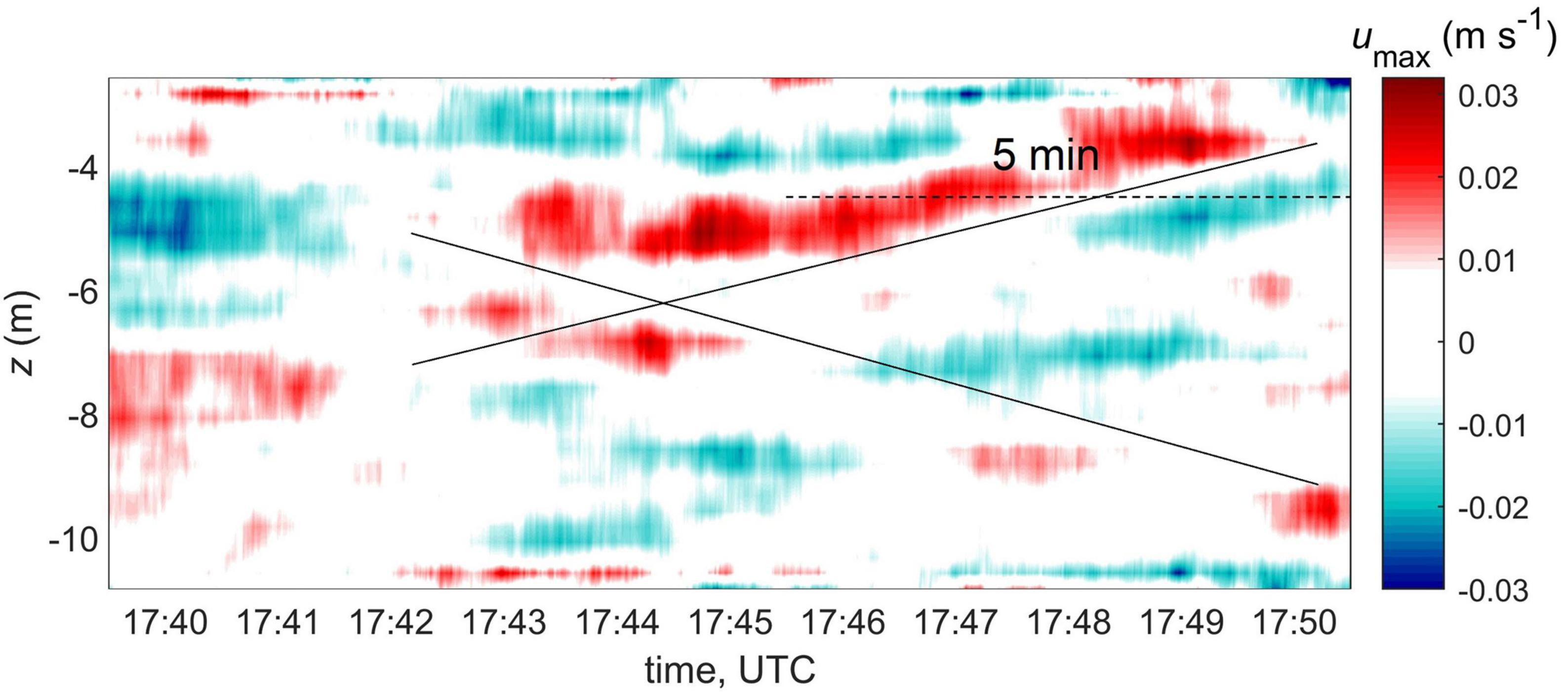
Figure 14. Band-passed maximum velocity component from ADCP data at station 12. Black lines show approximate direction of the internal wave phase propagation; dashed line indicates the internal wave period.

The strongest vertically propagating signal is seen at 17:45–17:50, z = −6 to –4 m. The lowest frequency wave shown in Figure 13 (k = 0.027 m^–1) has a wavelength of 233 m and a period of 5.1 min, roughly the same as the period of the perturbation in Figure 14. The horizontal velocity of this wave mode exhibits vertical shear at z = −6 to 4 m (similar to the observed), while the maximum vertical velocity occurs at z = −4 to 2 m (Figure 13B, blue profiles). Repeated MicroCTD salinity profiles (Figure 5) show vertical displacements of the pycnocline at 2–4 m depth at both frontal station 11 and 12, while inshore station 9 reveals neither such displacements nor elevated dissipation rates at the base of the plume. Although the data presented do not constitute an ultimate proof, they strongly suggest internal wave activity in the proximity of the interior front.

Discussion and Conclusion

In this study, we present observations of the WB plume formed by high freshwater discharge of O(1000) m³ s^–1 (all rivers combined) and a southwesterly upwelling-favorable wind acting continuously for ∼1.5 days prior to the survey. Such conditions, if the wind persists over several days, lead to the formation of cross-shelf plumes extending upstream and offshore as elongated “filaments” of buoyant water with minimal transvers spreading, as inferred from satellite images. The same feature appears to be present in observations reported here, where the freshwater content h_f remained nearly constant (∼0.8–0.9 m) over ∼20 km along the transect distance. The transect was aligned with the maximum offshore extent of the plume, as seen from Figure 2. This property contrasts the spreading of unforced supercritical plumes reported in modeling studies (e.g., Garvine, 1984; O’Donnell, 1990; Hetland, 2010) when the buoyant water spreads radially and the thinning of the buoyant layer does occur.

The observed plume comprises tidal pulses of different age distinguishable by their TS indices with older water being characterized by higher salinity and temperature. Tidal pulses are advected offshore and upstream by wind-induced currents, and are separated by interior fronts previously reported in Yankovsky and Voulgaris (2019). The present observations differ in that newer and older waters are separated not only in the horizontal but in the vertical as well with the newly released tidal plume spreading partially on top of the existing, previously released plume. This difference is likely caused by specifics of the wind forcing: in the present case, stronger wind stress was observed on the previous day, resulting in a deeper buoyant layer with lesser density anomaly. Vertical structures of velocity, salinity, and ε in the older (offshore) part of the plume imply that both the wind-induced shear stress and buoyancy (or, equivalently, pressure gradient force) affect plume spreading. However, stress divergence dominates in the upper part of the buoyant layer, while buoyancy is more pronounced in the lower part, with a velocity minimum found in the middle of the buoyant layer. This minimum velocity corresponds to the most homogeneous (with respect to the horizontal distance) part of the plume.

The observed plume is supercritical in the direction of the maximum depth-averaged velocity of the buoyant layer. In particular, for the observed interior front conditions, the backward propagating internal wave mode is not just reversed (as supercriticality implies) but is completely eliminated by the effect of the mean current shear. A supercritical regime in the plume can constrain the transverse spreading of the plume: since the interior front current flows in the upwind (i.e., downstream) direction, all pycnocline perturbations will ultimately radiate into the upwind edge of the plume and limit the plume’s downwind spreading. The source of internal waves is likely the newly released tidal pulse, although any non-stationary current within the plume can radiate waves. Internal waves can approach the interior front at an arbitrary angle, but they will experience strong refraction on the frontal current (e.g., Duda et al., 2018), with a fraction of the incident energy flux still escaping farther offshore. In this way, an interior front can trap a substantial fraction of the internal wave energy flux and direct it downstream.

Internal waves are ubiquitous in buoyant plume dynamics. Radiation of high amplitude internal solitons (of pycnocline depression) by supercritical tidally modulated buoyant discharges is well documented by both observational (e.g., Nash and Moum, 2005; Jay et al., 2009; McPherson et al., 2020) and modeling (e.g., Stashchuk and Vlasenko, 2009) studies. These solitons propagate through the previously existing buoyant layer and disintegrate into trains of high-frequency internal waves. Internal waves associated with buoyant discharge are reported even in non-tidal seas (Osadchiev et al., 2020) or in subcritical discharges (Mendes et al., 2021). Interior fronts with associated supercritical currents can fundamentally alter the fate of arriving internal waves and their ultimate dissipation.

In conclusion, the cross-shelf plume described in this study represents a distinctive regime of coastal buoyant plume dynamics, corresponding to conditions where a supercritical buoyant outflow is exposed to moderate upwelling-favorable wind. The superimposed wind-driven currents transport tidal buoyant pulses offshore and, in combination with buoyancy-driven circulation, maintain a supercritical regime of the resulting plume. Under these conditions, internal waves can contribute to mixing processes and the entrainment of the ambient shelf water at the base of the plume. Dedicated modeling exercise is the next logical step in delineating the outlined regime.

Data Availability Statement

Observational data presented in this study and a MATLAB code for solving the wave problem are available in Yankovsky et al. (2021); and https://zenodo.org/record/5796882. Auxiliary data are available at the following websites: VIIRS satellite images https://coastwatch.chesapeakebay.noaa.gov/region_cl.php; buoy wind data https://www.ndbc.noaa.gov/; tidal gauge data https://oceanservice.noaa.gov/facts/find-tides-currents.html; and freshwater discharge https://waterdata.usgs.gov/nwis/.

Author Contributions

DF, AY, and DC collected the data. DF preprocessed and archived the data set and estimated the TKE dissipation. AY analyzed the CTD and velocity data, solved the wave problem, and drafted an early version. DC processed the drone data. GV produced the SAR image. All co-authors subsequently discussed, revised, and edited the manuscript. All authors contributed to the article and approved the submitted version.

Funding

Data collection was supported by the Office of the Vice President for Research of the University of South Carolina through funding from the Advanced Support for Innovative Research Excellence (ASPIRE) program.

Conflict of Interest

The authors declare that the research was conducted in the absence of any commercial or financial relationships that could be construed as a potential conflict of interest.

Publisher’s Note

All claims expressed in this article are solely those of the authors and do not necessarily represent those of their affiliated organizations, or those of the publisher, the editors and the reviewers. Any product that may be evaluated in this article, or claim that may be made by its manufacturer, is not guaranteed or endorsed by the publisher.

Acknowledgments

Seamanship and enthusiasm of James Phillips, Captain of RV Coastal Explorer, are greatly appreciated. Gabby Ricche compiled a series of satellite images with corresponding forcing conditions for the Winyah Bay plume. We are indebted to reviewers and Steve Dykstra for their insightful comments and suggestions.

Footnote

1. ^ http://step.esa.int

References

Appendix

We consider small-amplitude perturbations in the x–z plane to the mean flow conditions described by the density and horizontal velocity profiles, ρ₀(z) and U(z), respectively. The linearized equations of momentum balance, mass balance and continuity are:

where u and w are the x- and z-components of the perturbed velocity vector, ρ is the perturbed density, p is the perturbed pressure, and t is the time. The system Equations A1–A4 can be reduced to the following equation for w:

where $N^2=-\frac{g}{{\mathrm{\rho }}_0}\frac{d{\mathrm{\rho }}_0}{dz}$ is the buoyancy frequency squared. We seek harmonic in time and in horizontal coordinate solution in the form:

where ω is the wave frequency and k is the wavenumber. Substituting Equation A6 into Equation A5 yields:

Here C = ω/k is the wave phase speed, and $\widehat{w}$ is subject to boundary conditions:

For a fixed value of C, Equations A7, A8 form an eigenvalue problem for k² with the vertical profile of the w-component being the corresponding eigenvector. The u-component profile can be recovered from Equation A4. The problem is solved numerically for the arbitrary profiles of N²(z) and U(z) by approximating derivatives with central differences. The problem is solved in MATLAB using its function eig. The accuracy of numerical solution was tested by using the analytical solution for constant N² and U. The dispersion curve ω = ω(k) for the gravest first mode is recovered by repeating calculations for different values of C. Equation A7 is analogous to the well-known Taylor–Goldstein equation for the stratified parallel shear flow, except here the solution is sought in terms of vertical velocity rather than streamfunction. It should be noted that in the present problem formulation, internal waves become non-dispersive at low frequencies, that is, their dispersion curve becomes a linear function with constant C. Thus, the solution technique which we use cannot be applied in this situation. However, at low frequencies the waves also become affected by the Earth’s rotation and so become dispersive again. In any case this low-frequency regime is beyond the scope of our study.

References

Atkinson, J. F. (1993). Detachment of buoyant surface jets discharged on slope. J. Hydraul. Eng. 119, 878–894. doi: 10.1061/(ASCE)0733-9429(1993)119:8(878)
Baines, P. G. (1995). Topographic Effects in Stratified Flows. Cambridge: Cambridge University Press, 482.
Branch, R. A., Horner-Devine, A. R., Kumar, N., and Poggioli, A. R. (2020). River plume liftoff dynamics and surface expressions. Water Resour. Res. 56:e2019WR026475. doi: 10.1029/2019WR026475
Duda, T. F., Lin, Y.-T., Buijsman, M., and Newhall, A. E. (2018). Internal tidal modal ray refraction and energy ducting in baroclinic Gulf Stream currents. J. Phys. Oceanogr. 48, 1969–1993. doi: 10.1175/JPO-D-18-0031.1
Filipponi, F. (2019). Sentinel-1 GRD preprocessing workflow. Proceedings 18:11. doi: 10.3390/ECRS-3-06201
Fisher, A. W., Nidzieko, N. J., Scully, M. E., Chant, R. J., Hunter, E. J., and Mazzini, P. L. F. (2018). Turbulent mixing in a far-field plume during the transition to upwelling conditions: microstructure observations from an AUV. Geophys. Res. Lett. 45, 9765–9773. doi: 10.1029/2018GL078543
Fong, D. A., and Geyer, W. R. (2001). Response of a river plume during an upwelling favorable wind event. J. Geophys. Res. 106, 1067–1084.
Fong, D. A., and Geyer, W. R. (2002). The alongshore transport of freshwater in a surface-trapped river plume. J. Phys. Oceanogr. 32, 957–972. doi: 10.1175/1520-0485(2002)032<0957:TATOFI>2.0.CO;2
García Berdeal, I., Hickey, B. M., and Kawase, M. (2002). Influence of wind stress and ambient flow on a high discharge river plume. J. Geophys. Res. 107:3130. doi: 10.1029/2001JC000932
Garvine, R. W. (1974). Physical features of the Connecticut River outflow during high discharge. J. Geophys. Res. 79, 831–846. doi: 10.1029/JC079i006p00831
Garvine, R. W. (1984). Radial spreading of buoyant, surface plumes in coastal waters. J. Geophys. Res. 89, 1989–1996. doi: 10.1029/JC089iC02p01989
Hetland, R. D. (2005). Relating river plume structure to vertical mixing. J. Phys. Oceanogr. 35, 1667–1688. doi: 10.1175/JPO2774.1
Hetland, R. D. (2010). The effects of mixing and spreading on density in near-field river plumes. Dyn. Atmos. Ocean 49, 37–53. doi: 10.1016/j.dynatmoce.2008.11.003
Hickey, B., McCabe, R., Geier, S., Dever, E., and Kachel, N. (2009). Three interacting freshwater plumes in the northern California Current System. J. Geophys. Res. 114:C00B03. doi: 10.1029/2008JC004907
Hickey, B. M., Peitrafesa, L. J., Jay, D. A., and Boicourt, W. C. (1998). The Columbia River plume study: subtidal variability in the velocity and salinity fields. J. Geophys. Res. 103, 10339–10368.
Horner-Devine, A. R., Jay, D. A., Orton, P. M., and Spahn, E. Y. (2009). A conceptual model of the strongly tidal Columbia River plume. J. Mar. Syst. 78, 460–475. doi: 10.1016/j.jmarsys.2008.11.025
Horstmann, J., Stresser, M., and Carrasco, R. (2017). “Surface currents retrieved from airborne video,” in Proceedings of the OCEANS 2017 – Aberdeen, Aberdeen, 1–4. doi: 10.1109/OCEANSE.2017.8084957
Huguenard, K., Bears, K., and Lieberthal, B. (2019). Intermittency in estuarine turbulence: a framework toward limiting bias in microstructure measurements. J. Atmos. Ocean. Technol. 36, 1917–1932. doi: 10.1175/JTECH-D-18-0220.1
Jay, D. A., Pan, J., Orton, P. M., and Horner-Devine, A. R. (2009). Asymmetry of Columbia River tidal plume fronts. J. Mar. Syst. 78, 442–459. doi: 10.1016/j.jmarsys.2008.11.015
Kakoulaki, G., MacDonald, D., and Horner-Devine, A. R. (2014). The role of wind in the near field and midfield of a river plume. Geophys. Res. Lett. 41, 5132–5138. doi: 10.1002/2014GL060606
Kastner, S. E., Horner-Devine, A. R., and Thomson, J. (2018). The influence of wind and waves on spreading and mixing in the Fraser River plume. J. Geophys. Res. Oceans 123, 6818–6840. doi: 10.1029/2018JC013765
Kim, Y. H., and Voulgaris, G. (2005). Effect of channel bifurcation on residual estuarine circulation: Winyah Bay, South Carolina. Estuar. Coast. Shelf Sci. 65, 671–686. doi: 10.1016/j.ecss.2005.07.004
Lentz, S. (2004). The response of buoyant coastal plumes to upwelling-favorable winds. J. Phys. Oceanogr. 34, 2458–2469. doi: 10.1175/JPO2647.1
Lentz, S. J., and Largier, J. (2006). The influence of wind forcing on the Chesapeake Bay buoyant coastal current. J. Phys. Oceanogr. 36, 1305–1316. doi: 10.1175/JPO2909.1
Li, C., Nelson, J. R., and Koziana, J. V. (2003). Cross-shelf passage of coastal water transport at the South Atlantic Bight observed with MODIS Ocean Color/SST. Geophys. Res. Lett. 30:1257. doi: 10.1029/2002GL016496
Lueck, R. (2016). Calculating the Rate of Dissipation of Turbulent Kinetic Energy. RSI Technical Note 028. Victoria, BC: Rockland Scientific International Inc.
MacDonald, D., and Geyer, W. R. (2005). Hydraulic control of a highly stratified estuarine front. J. Phys. Oceanogr. 35, 374–387. doi: 10.1175/JPO-2692.1
Mazzini, P. L. F., Chant, R. J., Scully, M. E., Wilkin, J., Hunter, E. J., and Nidzieko, N. J. (2019). The impact of wind forcing on the thermal wind shear of a river plume. J. Geophys. Res. Oceans 124, 7908–7925. doi: 10.1029/2019JC015259
McPherson, R. A., Stevens, C. L., O’Callaghan, J. M., Lucas, A. J., and Nash, J. D. (2020). The role of turbulence and internal waves in the structure and evolution of a near-field river plume. Ocean Sci. 16, 799–815. doi: 10.5194/os-16-799-2020
Mendes, R., da Silva, J. C. B., Magalhaes, J. M., St-Denis, B., Bourgault, D., Pinto, J., et al. (2021). On the generation of internal waves by river plumes in subcritical initial conditions. Sci. Rep. 11:1963. doi: 10.1038/s41598-021-81464-5
Münchow, A., and Garvine, R. W. (1993). Buoyancy and wind forcing of a coastal current. J. Mar. Res. 51, 293–322. doi: 10.1357/0022240933223747
Nash, J. D., and Moum, J. N. (2005). River plumes as a source of large amplitude internal waves in the coastal ocean. Nature 437, 400–403. doi: 10.1038/nature03936
O’Donnell, J. (1990). The formation and fate of a river plume: a numerical model. J. Phys. Oceanogr. 20, 551–569. doi: 10.1175/1520-0485(1990)020<0551:TFAFOA>2.0.CO;2
Osadchiev, A., Barymova, A., Sedakov, R., Zhiba, R., and Dbar, R. (2020). Spatial structure, short-temporal variability, and dynamical features of small river plumes as observed by aerial drones: case study of the Kodor and Bzyp River plumes. Remote Sens. 12:3079. doi: 10.3390/rs12183079
Spicer, P., Cole, K. L., Huguenard, K., MacDonald, D. G., and Whitney, M. M. (2021). The effect of bottom-generated tidal mixing on tidally pulsed river plumes. J. Phys. Oceanogr. 51, 2223–2241. doi: 10.1175/JPO-D-20-0228.1
Stashchuk, N., and Vlasenko, V. (2009). Generation of internal waves by a supercritical stratified plume. J. Geophys. Res. 114:C01001. doi: 10.1029/2008JC004851
Stewart, R. H., and Joy, J. W. (1974). HF radio measurements of surface currents. Deep Sea Res. Oceanogr. Abstr. 21, 1039–1049. doi: 10.1016/0011-7471(74)90066-7
Streßer, M., Carrasco, R., and Horstmann, J. (2017). Video-based estimation of surface currents using a low-cost quadcopter. IEEE Geosci. Remote Sens. Lett. 14, 2027–2031. doi: 10.1109/LGRS.2017.2749120
Wang, J., MacDonald, D. G., Orton, P. M., Cole, K., and Lan, J. (2015). The effect of discharge, tides, and wind on lift-off turbulence. Estuar. Coasts 38, 2117–2131. doi: 10.1007/s12237-015-9958-y
Whitney, M. M., and Garvine, R. W. (2005). Wind influence on a coastal buoyant outflow. J. Geophys. Res. 110:C03014. doi: 10.1029/2003JC002261
Wright, L. D., and Coleman, J. M. (1971). Effluent expansion and interfacial mixing in the presence of a salt wedge, Mississippi River delta. J. Geophys. Res. 76, 8649–8661. doi: 10.1029/JC076i036p08649
Xing, J., and Davies, A. M. (1999). The effect of wind direction and mixing upon the spreading of a buoyant plume in a non-tidal regime. Cont. Shelf Res. 19, 1437–1483. doi: 10.1016/S0278-4343(99)00025-4
Yankovsky, A. E. (2006). On the validity of thermal wind balance in alongshelf currents off the New Jersey coast. Cont. Shelf Res. 26, 1171–1183. doi: 10.1016/j.csr.2006.03.008
Yankovsky, A. E., and Garvine, R. W. (1998). Subinertial dynamics on the inner New Jersey shelf during the upwelling season. J. Phys. Oceanogr. 28, 2444–2458. doi: 10.1175/1520-0485(1998)028<2444:SDOTIN>2.0.CO;2
Yankovsky, A. E., and Voulgaris, G. (2019). Response of a coastal plume formed by tidally-modulated estuarine outflow to light upwelling-favorable wind. J. Phys. Oceanogr. 49, 691–703.
Yankovsky, A., Fribance, D., Cahl, D., and Voulgaris, G. (2021). Data for the Paper in Front. Mar. Sci. doi: 10.3389/fmars.2021.785967 (v1.0) [Data set]. Zenodo. doi: 10.5281/zenodo.5796882