
Machine learning (ML) employs algorithms and statistical models that enable computer systems to find patterns in massive amounts of data. They can then use a model that recognizes those patterns to make predictions or descriptions on new data.
Today, ML is used in virtually every industry, including retail, healthcare, transportation, and finance to improve customer satisfaction, boost productivity, and improve operational efficiencies. However, getting access to environments, which enables you to try out new tools and technologies, is often tricky at best, and prohibitive at worst.
In this post, I walk through each step to build an end-to-end ML service, starting from data processing to model training to inference, using RAPIDS. With the new one-click deploy feature of the NGC catalog, you can access the notebook and try out the ML pipeline, without having to spin up infrastructure and install packages yourself.
Accelerating application development with AI software and infrastructure
If you’re already building data science applications, you’re 90% of the way to using RAPIDS.
RAPIDS: Accelerating machine learning
RAPIDS is a suite of open-source software libraries that allows you to develop and execute end-to-end data science and analytics pipelines, entirely on the GPU. The RAPIDS Python API looks and feels like the data science tools that you already use, like pandas and scikit-learn, so you can reap the benefits with only minimal changes to your code.
RAPIDS eliminates bottlenecks in modern data science workflows by bringing data onto the GPU during ingestion directly and keeping it there for exploration, feature engineering, and model training. This allows you to iterate quickly through the early stages of the ML workflow, and try out more advanced techniques in fixed time on the GPU.
RAPIDS also integrates with other well-known frameworks, including XGBoost, which provides an API for carrying out training and inference with gradient boosted decision trees.
NGC catalog: A hub for GPU-optimized software
The NVIDIA NGC catalog provides GPU-optimized AI and ML frameworks, SDKs, and pretrained models. It also hosts example Jupyter Notebooks for a variety of applications including the example that I cover in this post. Now, the notebook can be easily deployed with a single click on Vertex AI Workbench.
Google Cloud Vertex AI: A GPU-accelerated cloud platform
Google Cloud Vertex AI Workbench is a single development environment for the entire data science workflow. It accelerates data engineering by deeply integrating with all the services necessary to rapidly build and deploy models in production.
NVIDIA and Google Cloud have partnered to enable this one-click feature that launches the JupyterLab instance on Vertex AI with an optimal configuration, pre-loads the software dependencies, and downloads the NGC notebook in one go. This allows you to start executing the code right away without needing any expertise to configure the development environment.
If you don’t have a Google Cloud account, sign up to receive free credits, which are sufficient to build and run this application.
Get building
Here’s every step you need to take to start your journey with GPU-accelerated data science.
Accessing the environment
Before you get started, make sure that the following prerequisites are met:
- You have registered for an NGC account, and signed in.
- You have registered for a Google Cloud Platform account, and have signed in.
After you sign into NGC, you are presented with the curated content.
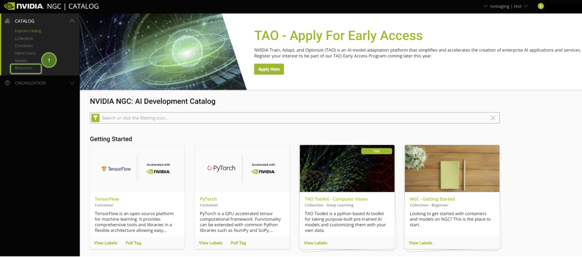
All Jupyter Notebooks on NGC are hosted under the Resources tab. Look at the Introduction to End-to-End RAPIDS Workflows. This page contains information on the RAPIDS libraries, as well as an overview of what is covered in the notebook.
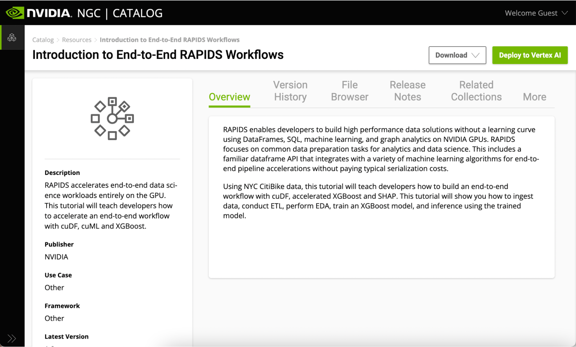
There are a couple of ways to get started using the sample Jupyter Notebooks from this resource:
- Download the resource
- One-click deploy to Vertex AI.
If you already have your own local or cloud environment with a GPU enabled, you could download the resource and run it on your own infrastructure. However, for this post, use the one-click deploy functionality to run the notebook on Vertex AI, without the need to install your own infrastructure manually.
The one-click deploy feature fetches the Jupyter Notebook, configures the GPU instance, installs dependencies, and provides running a JupyterLab interface to get started.
Setting up the managed notebook
Follow the brief tutorial to make sure that your environment is set up correctly.
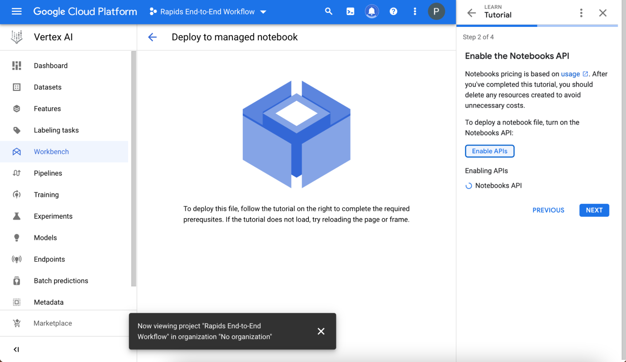
Create and name your project, and choose it in the Select a project field after the project is created. Write down the project ID value displayed automatically below the project name, as you need it later.
Next, enable the Notebooks API.
Setting up the hardware
Before you choose Create to deploy the notebook, choose Advanced settings. The following information is preconfigured but customizable, depending on the requirements of the resource:
- Name of the notebook
- Region
- Docker container environment
- Machine type, GPU type, Number of GPUs
- Disk type and data size
Before you deploy:
- Review to ensure that there are GPUs available in the region that have been preconfigured. If GPUs are unavailable, you see a warning and you should change your region:
- Make sure that the Install GPU driver for me automatically button is checked.
Now that everything looks good and you have your GPU and driver, choose Create at the bottom of the page. Creating the GPU compute instance and setting up the JupyterLab environment takes about a couple of minutes.
Starting Jupyter
Start the interface by choosing Open -> Open JupyterLab. The JupyterLab interface pulls the resources (custom container and Jupyter Notebooks) from NGC. The kernel may take a while to pull, so be patient!
When it’s loaded, you can select the RAPIDS kernel from the kernel selector. After the kernel has finished loading, in the left pane, double-click the notebook name.
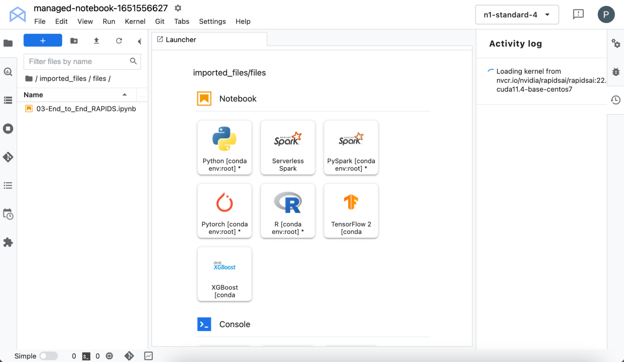
Without setting up your own infrastructure, you’ve now got access to a notebook environment with RAPIDS libraries preinstalled, so you can go ahead and try it out for yourself.
Working with the workflow
The project uses data from the CitiBike bike share program in New York City. More details are available in the notebook itself.
Before you dive into data processing, you can look at the details about the GPU using the NVIDIA SMI command. This shows you what you expected: VertexAI has allocated a V100 T4 GPU, with 16 GB of memory.
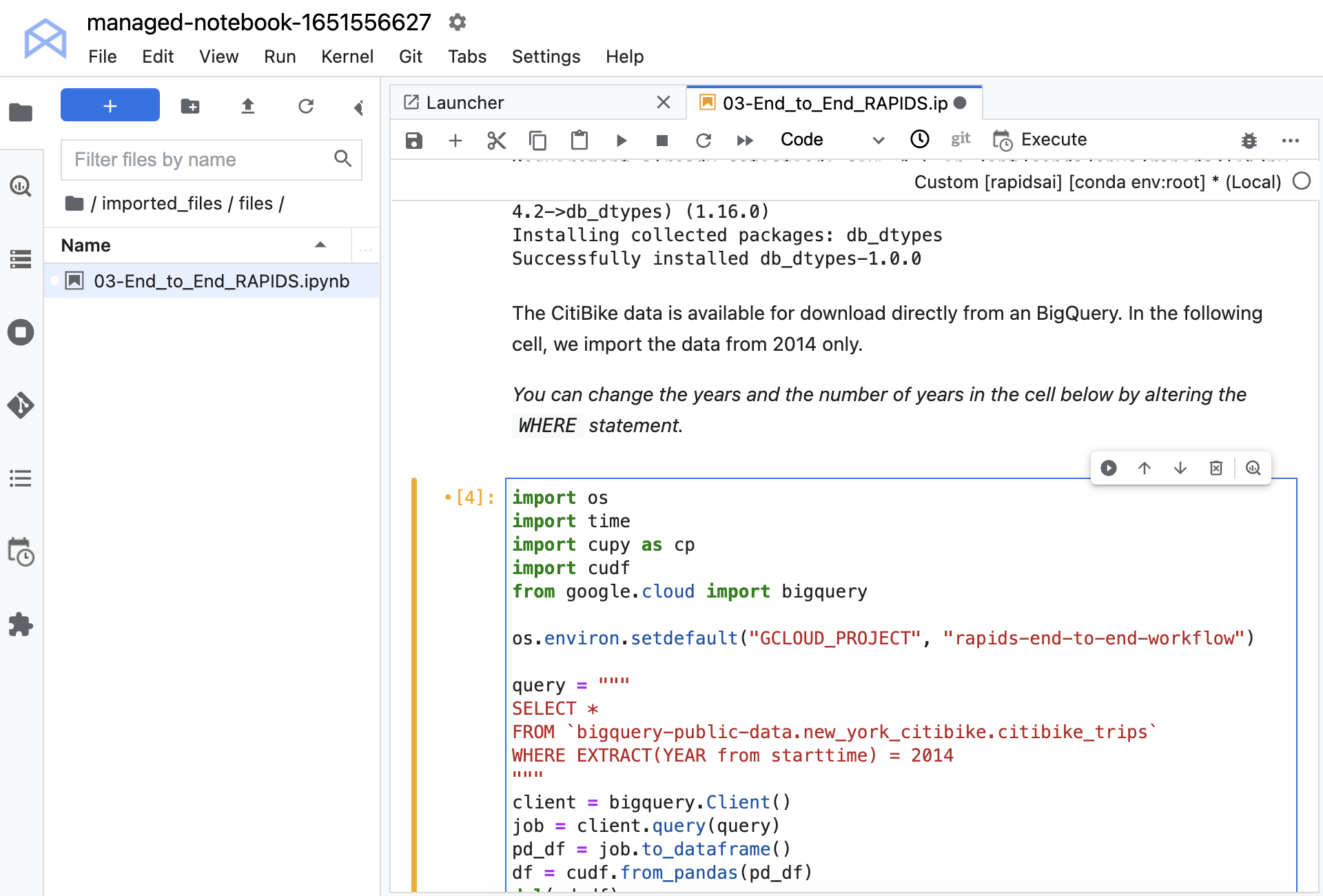
You must install a couple of libraries, which enable you to load your data from Google BigQuery. This data set is publicly available on BigQuery, so you don’t need any credentials to load it. Load the data from a large query, using the Python API.
Convert the data into a cuDF data frame. cuDF is the RAPIDS GPU DataFrame library, which provides everything you need to efficiently transform, load, and aggregate data on the GPU. The cuDF data frame is stored on the GPU, and that is where the data remains for the rest of the work. This helps provide massive speedups by leveraging the speed of GPUs and cutting down on costly transfers back and forth from CPU to GPU.
Before you can run the notebook, uncomment the command os.environ.setdefault and put the ID of your project into the second argument. If you don’t remember the ID assigned to your project when you set it up, it’s shown on the Workbench main page after you select a project. Remember to use the ID and not the name.
Now, the data is loaded. You can inspect it and look at data types and summaries of the features. Each entry contains a start time, stop time, station ID denoting where the bike was collected, and station ID denoting where the bike was dropped off. There’s also other information about the bike, pick up and drop off location, and the user’s demographics.
Data processing
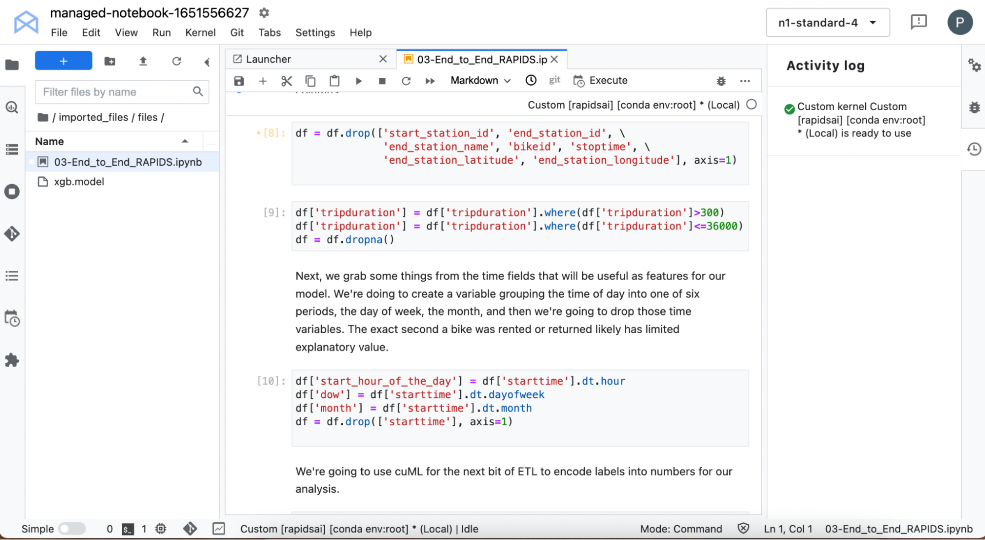
In the next cells, you process the data to create feature vectors, which capture the important information to use to train the ML model.
Process the start time to extract information such as the day of the week that the bike was hired, as well as the hour of the day. You remove all features from the data, which contain information about the end of the ride, as the goal is to predict the ride duration at the point of pick-up.
You also filter out extremely short rides for faulty bikes immediately returned and extremely long rides lasting more than 10 hours. The city bikes are supposed to be used for relatively short trips around the city and are not suitable for long journeys, so you don’t want this data to skew the model.
Use some of the cuDF built-in time functionality to capture specifics about when the bikes were checked-out. Do some other data processing, like using cuML to automatically create label encoding for certain text variables.
Model training
You then train an XGBoost model. XGBoost provides an API for carrying out training and inference with gradient-boosted decision trees.
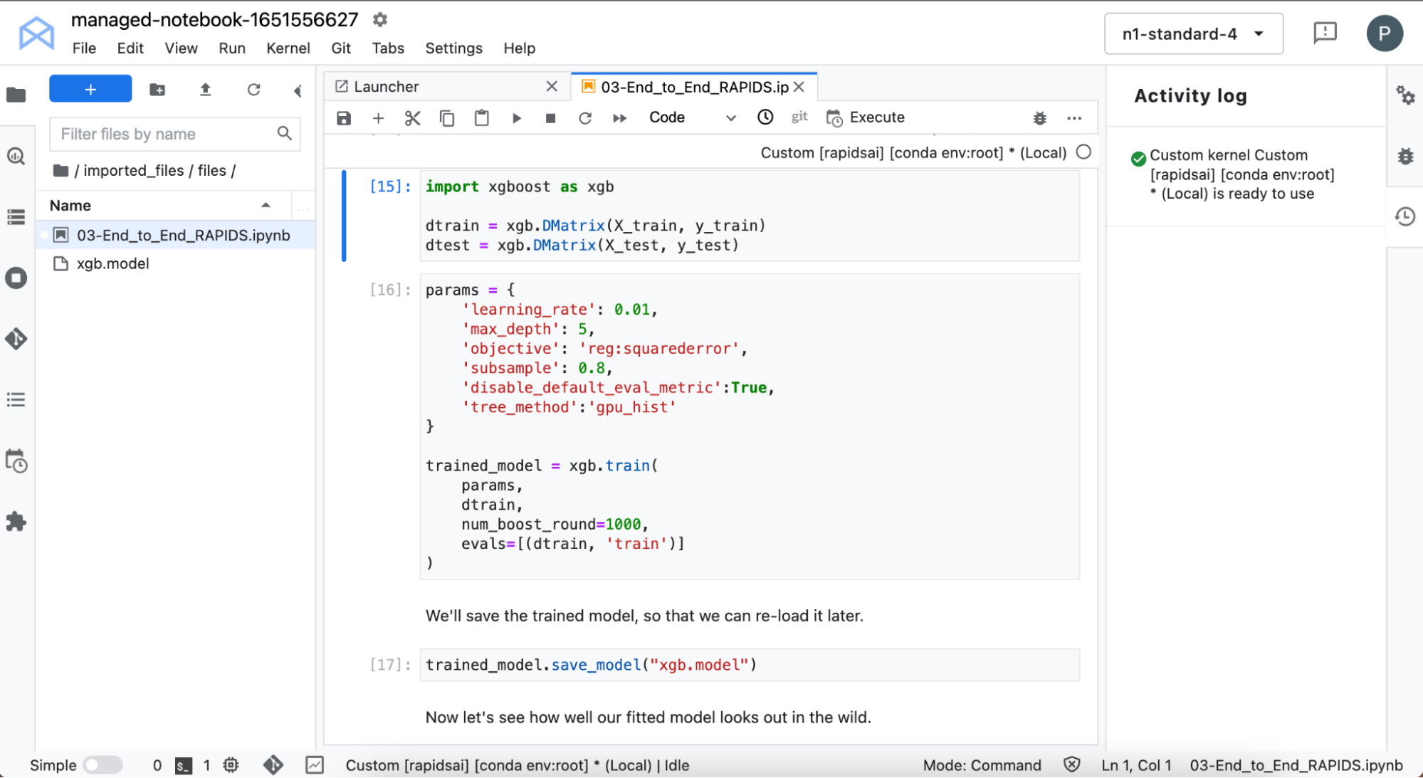
This is training on the GPU: super fast. It accepts your data directly from cuDF with no need to change the format.
Now that you’ve trained the model, use it to predict ride time on some data that it wasn’t trained on, and compare that to the group truth. Without tuning any hyperparameters, the model is doing a reasonable job at predicting ride time. There are improvements that could be made, but for now look at which features are influencing the model’s predictions.
Model explanation
When using complex models, such as XGBoost, it’s not always straightforward to understand the predictions made by the model. In this section, you use SHapley Additive exPlanation (SHAP) values to gain insight into the ML model.
Computing SHAP values is a computationally expensive procedure, but you can accelerate the procedure by running on NVIDIA GPUs. To save more time, compute SHAP values on a subset of the data.
Next, look at the influence of individual features, as well as combinations of features.
Accelerating inference
Training the model is often seen as the computationally expensive part of the workflow, so GPUs come into their own here. In practice, that’s true. But GPUs can also dramatically accelerate the time it takes to make a prediction for some models.
Reload the model because XGBoost caches previous predictions and time it when making predictions on both CPU and GPU.
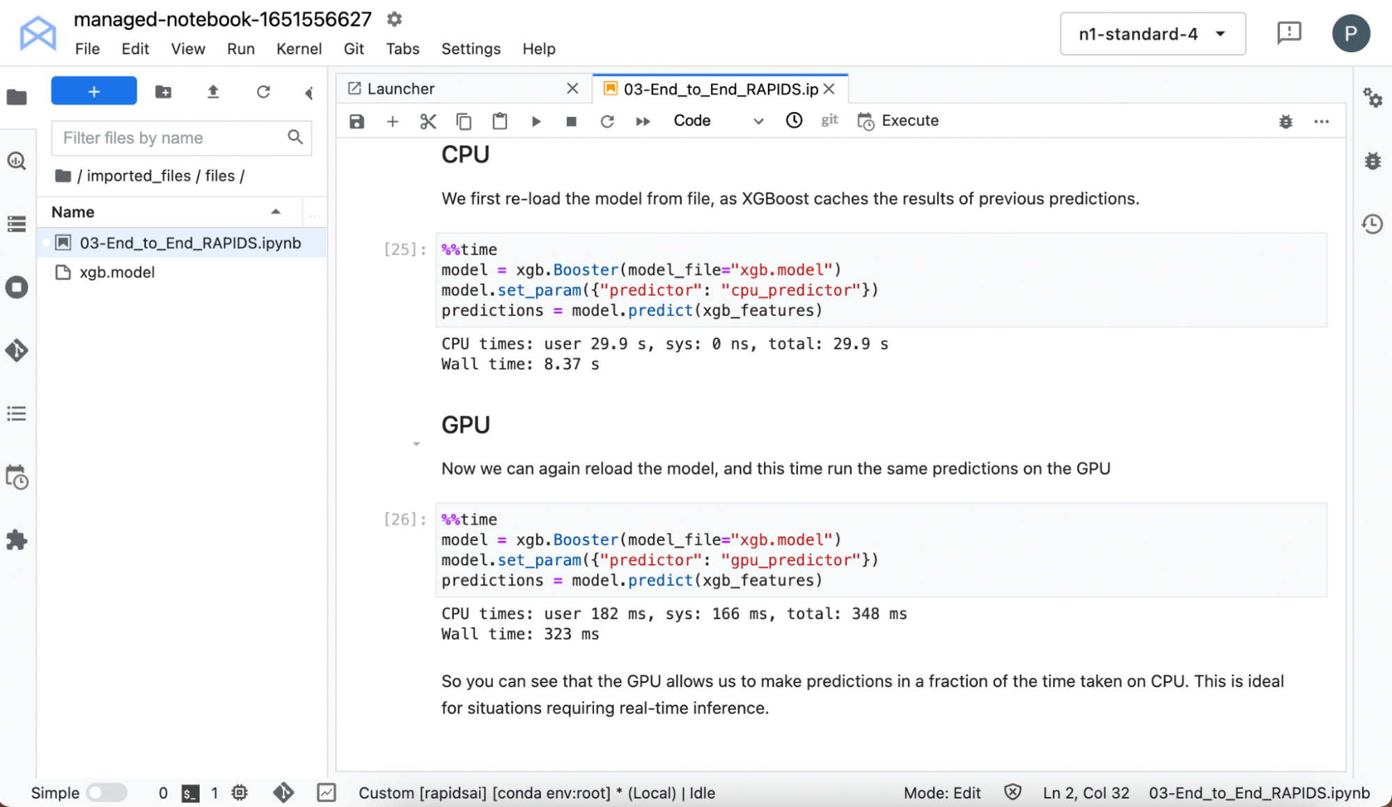
Even on this small data set and simple model, you can see the massive speedups in inference when running on the GPU.
Conclusion
RAPIDS enables you to carry out end-to-end workflows on the GPU, giving you the power to consider more complex techniques and gain quicker insight into the data.
With the NGC catalog’s one-click deploy feature, you can get access to an environment with RAPIDS in a matter of minutes and develop your ML pipelines without having to spin up your own infrastructures or install the libraries yourself.
It’s easy to get started! Follow these steps and you’ll be on your way to speeding up all your data science work without any of the hassles of setting up infrastructure.
To learn more about RAPIDS and reach out to the RAPIDS team on Twitter. And of course, search through the NGC catalog to get more easy-to-deploy models and examples.