
The guide
for users of the ARIES for SEEA Explorer
I. The ARIES for SEEA application
The ARIES for SEEA Explorer is a web-based application built on the k.LAB Integrated Modelling Platform. The application has access to all information (data and models) available on the Integrated Modelling network, and provides a dedicated user interface to easily compile accounts within the UN System of Environmental-Economic Accounting (SEEA).
ARIES for SEEA can also be accessed via software download for recurrent users, for better performance in terms of speed and computation capacity. More info at https://integratedmodelling.org/getting-started/
1.1 Spatial and temporal context of the analysis
At the top of the menu on the left side of the screen, you can specify the geographic area and temporal and spatial scale.
1.1.1 Where
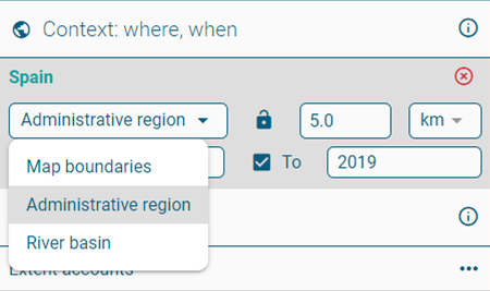
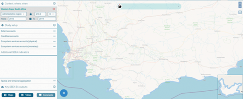
At the top of the panel, a drop-down menu provides three options to select an analysis context by zooming and panning on the map. When the “administrative regions” or “river basin” option is chosen, the currently highlighted context will be outlined in light blue.
- Map boundaries: Select an area of interest by panning and zooming in/out. The entire area visible on the screen becomes your analysis context.
- Administrative regions: This option automatically identifies the largest administrative entity (e.g., Country or Subnational Unit) in the area selected, according to the M49 standard endorsed by the UN. By zooming in, the user can choose a smaller administrative region. We recommend this option for novice users, as it offers a simple way to identify standard administrative boundaries for ecosystem accounting.
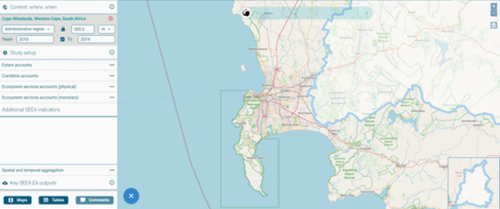
- River basin: This option selects an area of land draining to a specific water body based on FAO Hydrological Basins (simplified).
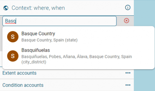
- Alternatively, the user can also directly type the name of a geographical context (i.e., country, region, city, or other geographic entity) in the ARIES for SEEA Search bar, starting with a capital letter.
These names are queried from the OpenStreetMap (OSM) database. Users should be aware that OSM boundaries may differ slightly from those selected using the “Administrative regions” option of the drop-down menu.
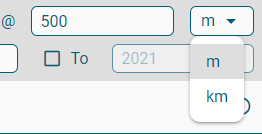
1.1.2. Resolution
The user can select the spatial resolution for analysis, and choose between meters or kilometers.
If a resolution is chosen that is higher than that of available input data, ARIES will compile accounts at the resolution of the finest grained available data.
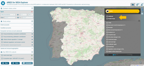
1.1.3. When
Select the year(s) for your analysis. If data are missing for a specific year of interest, ARIES automatically fills gaps using the closest available year’s data.
I. Single-year analysis (uncheck the box)
![]()
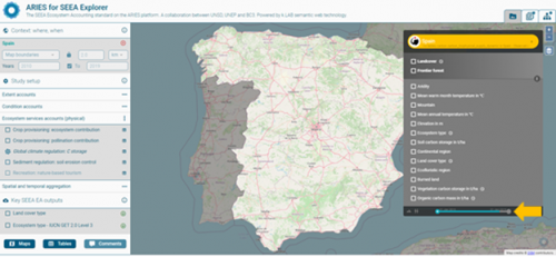
II. Multi-year analysis – showing change over time (check the box)
![]()
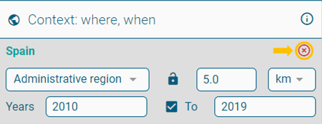
1.1.4. Reset
The red “X” button on the upper right can be used to reset a previously selected context, or to stop a computation in progress (all computed results will be lost).
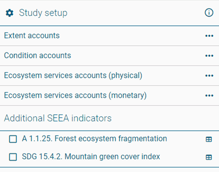
II. Study setup
Each account contains a drop-down menu (three horizontal dots), from which the user can select accounts to compile:
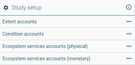
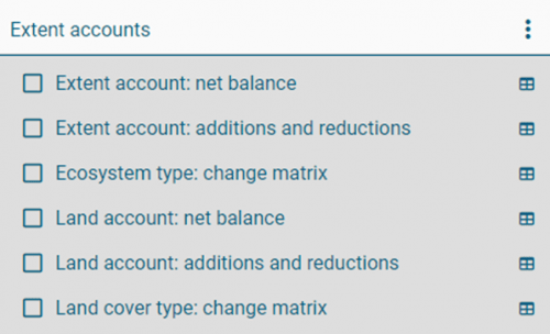
2.1. Extent Accounts
These accounts measure the extent of the IUCN Global Ecosystem Typology ecosystem types, or land cover, present in the context of your analysis, in km2.
The different types of accounts provide varying levels of detail in summarizing ecosystem/land cover extent and its change over the selected time period.
2.2. Condition Accounts
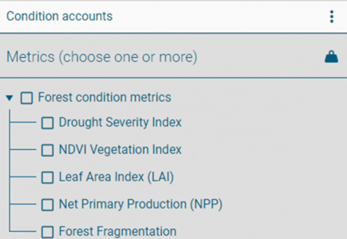
These accounts measure ecosystem condition. Currently, only forest ecosystem condition accounts are supported, but condition accounts for other ecosystem types will be added soon (beginning with those for grasslands).
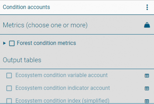
The conditions metrics available for inclusion in the account appear in a drop-down menu when the user clicks on the triangle next to “Forest condition metrics”.
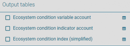
Three types of ecosystem condition accounts are available:
- Condition Variable Account: report the value of each condition metric in their originally observed values (non-transformed).
- Condition Indicator Account: rescale ecosystem condition variables to values between 0 and 1. Rescaling is calculated as the difference between the observed condition variable value and the optimal condition reference.
By normalizing multiple condition variables, different indicators can be more directly compared; - Condition Index Account: combines all indicators together using a weighted mean. Currently, all indicators take the same weight, summing to 1 (e.g., 0.25 when four condition metrics are selected). In future releases of ARIES for SEEA, users will be able to assign custom weights to the indicators to better reflect their local importance when accounting for ecosystem condition.
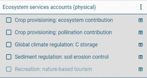
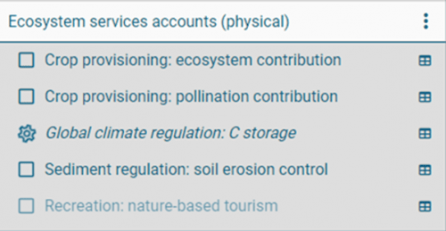
2.3. Ecosystem services account (physical terms)
These accounts measure the biophysical quantities of services provided by ecosystems and used by economic units. Use tables are not explicitly supplied with the model outputs, but use is described in the automatically generated reports for the selected accounts. In the current version, four ecosystem services are available. A fifth one, Nature-based tourism, is in its final stages of development and will be made available in a future ARIES for SEEA release.
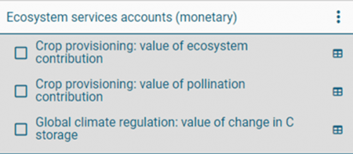
2.4. Ecosystem services account (monetary terms)
These accounts measure the monetary value of the selected ecosystem services, applying SEEA EA-compliant valuation method(s). Use tables are not explicitly supplied with the model outputs, but use is described in the automatically generated reports for the selected accounts. In the current version, three ecosystem services are available. A fifth one, Nature-based tourism, is in its final stages of development and will be made available in a future ARIES for SEEA release.
2.5. Spatial and temporal aggregation
The user can select how the results of the accounts are aggregated in accounting tables.
Currently, only the first option is available. In future ARIES for SEEA releases, the user will be able to generate accounting tables as follows:
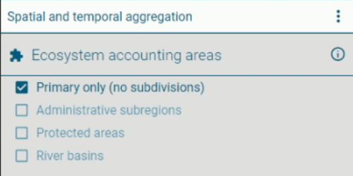
- “Primary only”: a single table summarizing results for the entire context identified by the user;
- Administrative subregions: multiple tables grouped by subnational jurisdictional entities (i.e., administrative level 1 – State, Province, or District);
- Protected areas: multiple tables grouped for protected areas found in the analysis context;
- River basins: multiple tables grouped results by watersheds found within the analysis context.
2.6. Temporal accounting
When a multiple-year analysis is selected, the user can decide to output tables:
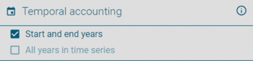
- For the first and last years of the time series only, or
- For all years within the time period selected.
III. Key outputs and observations
This section shows the most relevant spatial inputs and outputs in the account(s) run by the user
(e.g., in the case of ecosystem extent, the most relevant outputs are land cover and ecosystem type data).
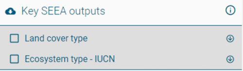
The last section stores all tables and maps produced in that session, so that the user can download them in a zipped file (of Excel spreadsheets or GeoTIFFs) before leaving the application.

In the upper left corner of the application, there is a section dedicated to SEEA-relevant indicators.

This section includes selected indicators from the Sustainable Development Goals (SDGs) and the Convention on Biology Diversity (CBD) Post-2020 Biodiversity Indicators, which have been added to the application.
Once it is opened, a drop-down menu shows the list of available indicators.
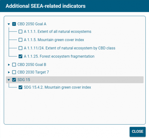
Those selected by the user are added in the ARIES for SEEA panel as if they were an additional standard SEEA EA account
IV. Quick tips
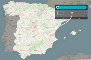
4.1. Set your context
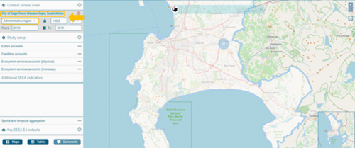
(e.g., Cape Town in South Africa). Suggested way:
- Zoom and pan using the Map boundaries option:
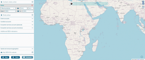
- Make sure the screen contains your target context:
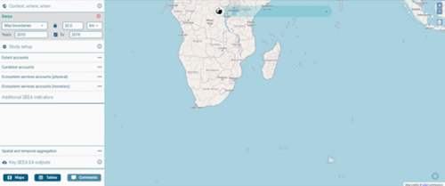
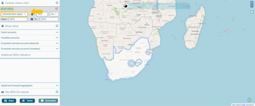
- Once the screen contains the area of interest, switch to Administrative region:
- If the whole administrative region does not fit the screen, a locator map in the lower-right corner of the interface will show the entire context as currently selected:
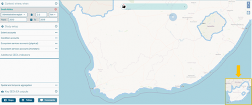
- Refine your search further (zooming in/out) to make sure the desired region is selected:
- Note: the region automatically selected is not always the most central, but part of the screen occupying the largest area:
- The name of the geographic entity is displayed on the upper left side of the application:
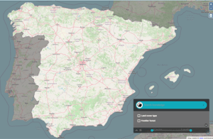
4.2. Spinning gear
When the gear starts spinning, the system is computing the model(s) requested by the user:
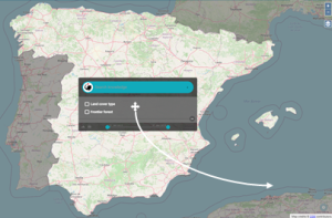
To offer the best visualization of the context in analysis, the search bar/results box can be positioned where the user prefers. To do so, point the cursor over the search bar, and once this symbol ![]() appears, drag it to a preferred location.
appears, drag it to a preferred location.

V. Explore results and methods used to run your accounting models
Aspects of the user interface change once you begin to run an accounting model:
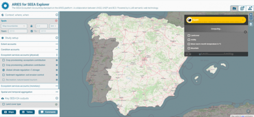
5.1. Run an accounting model
(e.g., ecosystem extent account – simple net balance).
Once the extent account is selected, the search bar will turn yellow.
A rotating gear will appear next to the selected account(s), which indicates that the model is being compiled.
When a model input or intermediate output has been computed, it is listed and can be explored individually, by selecting the specific layer (e.g., aridity):
When a main output of the model is computed, this is listed (in the darker section) above the other inputs/intermediate output:
If the model is dynamic (i.e., is calculated for >1 year), the progress bar at the bottom of the search bar/results box progresses as the computation continues:
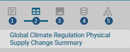
In the right-upper corner of the app, three tabs are now available:
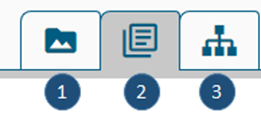
- Data view (always available)
- Documentation view
- Data flow view
In our example, the application automatically takes the user to the section showing the accounting result(s).
This happens every time a final outcome is generated:
To review other sections of the documentation:
5.2. The report
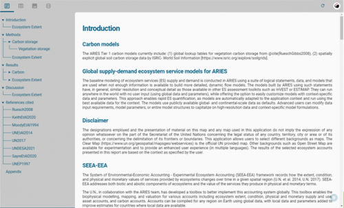
The tree-menu on the left facilitate the navigate of the information reported. Each report includes:
- A general introduction to the model(s);
- Information on the SEEA framework or any other more general modeling frameworks (when part of a larger set of models);
- The methods applied;
- A summary of the main results;
- Caveats or other considerations in interpreting model results, as part of the discussion; and
- Reference(s) for data and method(s) used.
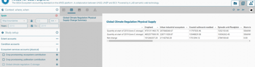
5.3. Tabular results
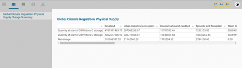
To ease the observation of the results:
- The first column is visible while scrolling to the right,
- Results can be sorted by the element in the first column, or by ascending and descending order of the result of any column
- The size of the text can be adjusted using the buttons in the upper right (with yellow circles)
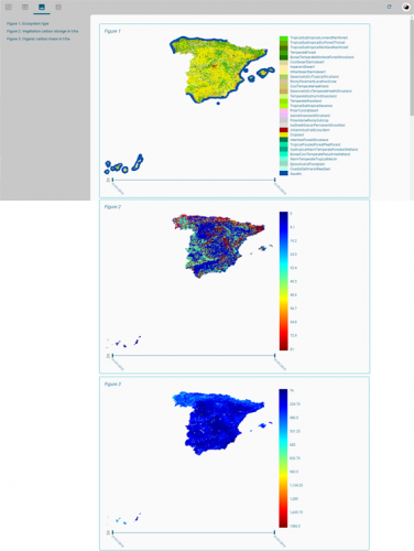
5.4. Image(s) section
Figure(s) and (maps) generated during the computation are listed in this section and can be explored individually.
If results come from multi-year models, the maps are interactive and shows changes over time.
5.5. Resources section
Lists all the resources used in the computations, to provide full-transparency on the final output.
Each of the data resource can be explored individually.
5.6. Dataflow section
Shows a list containing a visual summary of each model component and how these were combined to obtain the final results. In the next version of ARIES for SEEA, this section will also report the decisions taken by the system on:
- Which combination of data and models was implemented,
- Which data and model alternatives could have been used instead and,
- The AI parameters used to support the choices made.
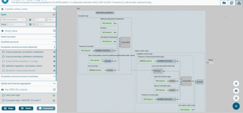
5.7. Dataflow view
The third tab available once a model has run is the Dataflow view.
This shows a diagram that visually summarize each model component and how those were combined to obtain the final result(s). Clicking on an individual rectangle provides details about the dataset, algorithm, etc. used at each step of the model.
VI. Spatialization of statistical aggregates
This subsection explains how ARIES spatializes tabular national statistical data and aggregates it through spatial modelling, using crop provisioning as an example. The problem can be framed as follows:
- National statistical aggregates provide national-level crop production data in a particular year.
- For SEEA EA accounting, we also need to map production levels.
- Spatial data (maps) identifying production of most cultivated crops are available, but often for a limited number of years, not in time series, and at coarse spatial resolution. Such data are typically generated using subnational agricultural production data correlated spatial data (e.g., for land cover or crop locations).
The method implemented follows:
- Spatially explicit crop production data (3) identify where production for a certain crop occurred in a given reference year (e.g., 2010);
- We overlay spatially explicit crop production data (3) with national boundaries to calculate a crop production reference table for each country (1) and crop. The reference table (1) enables us to:
- Account for changes in political borders;
- Disaggregate production coming from overseas departments/regions included in national statistics (3); and
- Reliably produce results at scales aside from national scale (i.e., subnational, supranational)
- The spatialization of the production coming from statistical aggregates (4), is thus based on the information on (1), (2) and (3), as shown in the graphic below:
Example of spatial disaggregation: crop production
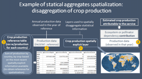
(1): Production table (reference)
(2): Production data from statistical aggregates (in reference year)
(3): Crop production map (spatial data in reference year)
(4): Production data from any year
Note that 2 and 4 must come from to the same data source (apply the same methodology), in order to generate spatialized crop production in time series.
The models only estimates the reallocation of such production, the biophysical production comes from statistical aggregate
This approach assumes crop extent to be constant (based on spatial data for the reference year), with only crop yield (tons produced per hectare) changing over time – an assumption we know to be false, but that a lack of time series spatial data based on subnational crop production forces us to accept, for now. Increases or decreases in production are thus spread across the whole country, rather than for that specific (but unknown) areas. The approach can be improved significantly with:
- More up-to-date spatially explicit data on crop production; and
- Statistical aggregates from higher-level administrative units (i.e., at state, region, province, or district level).
- Such approaches can enable the use of methods that produce more accurate spatial disaggregation of any statistical aggregates.
VII. Other ARIES features
While most of the functions needed to compile SEEA accounts are available through ARIES for SEEA interface, the normal functionalities of the ARIES Explorer remain available through the search bar.
This sections shows how to query them.
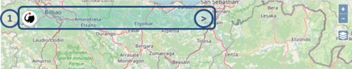
7.1. Search the knowledge bar (1)
This box is used to call models, select your context, modify default settings, and show the help page.
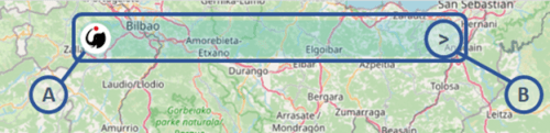
- Query an observable from the space bar (A):
Please note: unlike the search bar in the ARIES for SEEA application, the general ARIES Explorer search bar is case-sensitive.
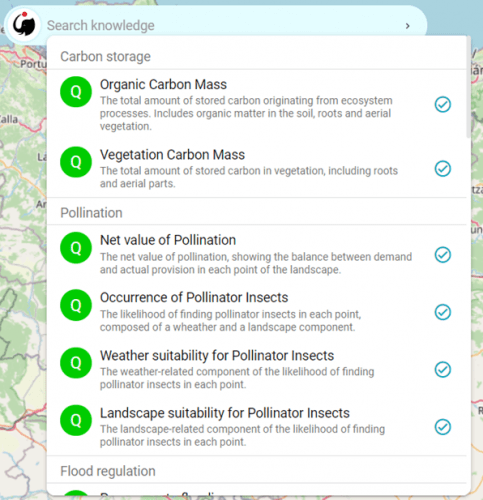
Press the space bar on the empty box to receive suggestions:
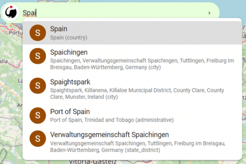
Start with an upper-case letter to search for a geographical context (invalid if you have already set a context):
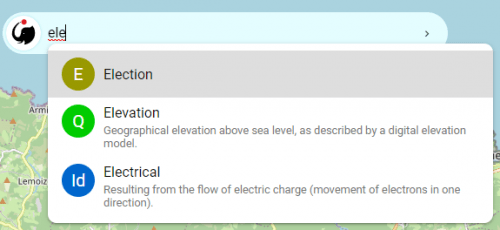
Start with a lower-case letter to search for an observation (e.g., elevation):
- Other settings/options/help (B)
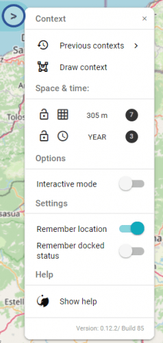
Context:
- Reset a previously used context;
- Draw a new context (using your cursor).
Space and time:
- Adjust the spatial and/or temporal resolution of your analysis.
Options:
- Activate the interactive mode to add manually add input to the model (adjusting parameter values).
Settings:
- Remember location (remember the last context selected);
- Remember docked status.
Help:
- Show the help tutorial.
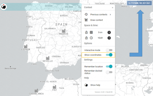
- New option to show the coordinates of your cursor (they change as you move it around)
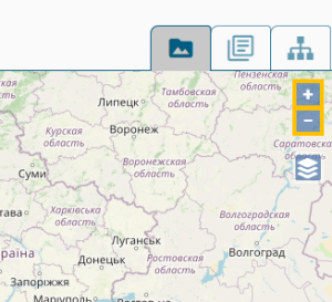
7.2. Zoom (2)
Zoom in (by clicking on the ![]() ) and out (
) and out (![]() ). This can be useful when selecting your context using map boundaries (entire rectangle shown in the interface) or administrative regions or river basins, which change as a user zooms and pans the map.
). This can be useful when selecting your context using map boundaries (entire rectangle shown in the interface) or administrative regions or river basins, which change as a user zooms and pans the map.
7.3. Background map (3)
Select the background map you prefer. By default, ARIES uses OpenStreetMap as it currently offers the best user experience even at higher resolutions.
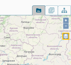
The user can switch to other available background maps as desired.
VIII. Coming soon
Additional features that will be made available in future releases of ARIES for SEEA include:
- Various improvements to ecosystem condition accounts:
- Option to select multiyear averages rather than single opening and closing years
- Custom weighting of metrics for ecosystem condition index accounts
- Handling presence/absence and categorical data in ecosystem condition accounts (e.g., burned area)
- Incorporation of other SEEA-related indicators, such as those from the SDG and CBD frameworks
- Physical and monetary supply-use accounts for nature-based tourism
- Reporting by administrative subregions, protected areas, and watersheds as ecosystem accounting areas
- Various “interactive mode” options for user to supply model inputs and parameters
- Improved integration of user-supplied spatial data inputs through a drag-and-drop interface
- Various improvements to functionality and user experience
IX. Training programs and material
Coming soon.